tions from the given final condition. If the number of im- pulse functions which depend on the number of the state variables is large, this search procedure may become pro- hibitively tedious.

The present method can be used to handle most of the constraints and performance indexes encountered in ordi- nary optimum design problems. For a detailed discussion of these problems the reader is referred to the paper by Rozonoer (6) . The method offers some possibilities for use for on-line optimizing control of a process. A special purpose analogue computer could be built for this use.

The analogue computer is ideally suited for solving two point boundary value problems. However for more com- plicated problems where frequent rescaling and fairly high accuracy is desired, a combined analogue-digital com- puter would present many advantages. The optimum gradients of temperature, pressure, and concentrations of certain chemical species in a chemical reactor are being investigated by the use of a combined analogue-digital computer.

ACKNOWLEDGMENT

The author is indebted to the Phillips Petroleum Company for permission to publish this paper. He also wishes to thank Mr. R. T. Brashear for his help in using the analogue simulator and Mr. L. R. Freeman for his many helpful discussions.

NOTATION

El , Ez = activation energies of the first and second reac-

G Gi, Gz = frequency-factor constants in 4rrhenius equa-

H = Hamiltonian function

tions = mass flow rate, g./min.

tions

ki, kz = reaction rate constants of the first and second

N = total moles ni, nz = moles of A and B, respectively pi, . . ., pn = impulse functions R = gas constant T = temperature t = independent variable ui, . . . Ur = control variables xi, . . ., xn = state variables x rr = total pressure, atm. Ti, rrz = partial pressures of A and B , respectively, atm.

LITERATURE CITED 1. Bellman, R., “Adaptive Control Processes: A Guided

Tour,” Princeton University Press, Princeton, New Jersey (1961).

reactions

= length parameter of the reactor, liter

2. Brooks, Samuel H., Operations Research, 7, 430 (1959). 3. Ibid., 6, 244 ( 1958). 4. Favreau, R. R., and R. Franks, Paper presented at the

Second International Conference for Analog Computation, Strasbourg (September, 1958).

5. Satterthwaite, F. E., Rept. #10/10/59, Statistical Engi- neering Institute, Wellesley, Massachusetts.

6. Rozonoer, L. I., Automation and Remote Control, 20, 1288, 1405, 1517 (1959).

7. Pontryagin, L. S., Automation Express, 1, 15, 26 (1959). 8. Boltyanski, V. G., R. V. Gamkrelidge, E. F. Mischenko,

and L. S. Pontryagin, “Proceedings of the First Interna- tional Congress of the I.F.A.C.,” Moscow, U.S.S.R. (1960).

9. Munson, J. K., and A. I. Rubin, Paper presented at Na- tional Simulation Conference, Dallas, Texas ( 1958).

10. Bilous, O., and N. R. Amundson, Chem. Eng. Sci., 5, 81, 115 (1956).

11. Aris, R., ibid., 13, 18 (1960).

1963; paper accepted Septembm 11 Automatic Control Conference, MinnedpoIis, Minnesota.

Manuscript reveived July 24 1963; revision received September 9, 1963. Paper presented at Joint

A Model Chemical

Building Technique for

Engineering Kinetics WILLIAM G. HUNTER and RElJl MEZAKI

University of Wisconsin, Madison, Wisconsin

The object of much experimentation is to build or discover a suitable model for a given system. Unfortunately very little work has been published on what constitutes good strategies in these situations. This paper i s an attempt to formulate an approach to this important prob- lem of iteratively improving models in the area of chemical engineering kinetics. In this technique a statistical analysis is applied to the estimated parameters of a tentatively entertoined theoret- ical model in such a way as to pinpoint its inadequacies, i f they exist, so that it i s possible to proceed in a logical manner to an appropriate modification of this model. This modified model i s then analyzed in a similar way, and further modifications are suggested. In general the cycle is repeated as often as is necessary to reach an adequate model. This sequential method is illustrated by finding an adequate reaction model for the total catalytic oxidation of methane.

A simple method for iterative model building has re- cently been described ( 4 ) in which a statistical analysis is applied to the estimated parameters of a theoretical model rather than to the original observations themselves. By adopting this method it should be possible to pinpoint

inadequacies of a given model in such a way as to sug- gest specific ways in which the model can be modified, if necessary, to yield a more useful one. The purpose of this paper is to apply this technique for mode1 building to some kinetics data on the catalytic oxidation of methane

Vol. 10, No. 3 A.1 .Ch.E. Journal Page 315

and to indicate how the method might be applied to other problems of this kind. Specifically it is shown how one can proceed in a sequential manner, starting with a tentative theoretical model for the reaction, and be led in a logical way to appropriate modifications of this original formula- tion.

Such a systematic analysis of kinetics data is desirable particularly in situations similar to the one discussed here where no fewer than eighty mechanisms were put for- ward as possible. One method of approach would be to examine each of these models individually and select the best one, but there are two obvious drawbacks: it will be extremely time consuming to check each of these models carefully, and even then the most appropriate model may not be contained in this original set.

The iterative method for model building helps on both counts. Since some of the models, a priori, will be more likely to be correct, it will often be possible to start with one of them and by proper analysis be guided to the best model in the set. Moreover the analysis may lead to a particular modification of the original model that is out- side the original set; that is, that has been overlooked in the initial cataloguing of possible models.

The method of analysis is based on the principle that constants should stay constant. The basic idea can be il- lustrated by considering a simple kinetic example where the model being entertained is the first-order decomposi- tion of a chemical substance 7):

The rate constant 8 in this model should not be a func- tion of the initial concentration of 7. This fact immediately suggests one obvious way to check the adequacy of the mathematical model. For each of a number of initial con- centrations [y]o measurements of [v] could be taken at different times t, and the rate constant 8 could be esti- mated by the method of least squares or some other ap- propriate means. It should then be possible to examine

the set of estimated values 3 to determine whether they remained constant within experimental error or on the other hand whether they exhibited a dependence on the initial concentration. If the former were true, then there would be no reason to doubt the adequacy of the pro- posed model, at least insofar as this particular aspect of the data were concerned. If the latter were true however, then the model would be shown to be inadequate and would have to be modified in a suitable manner depend-

ing upon the way in which 5 depended on [710. In such a simple situation the experimenter usually

finds an adequate model by an informal trial-and-error procedure in which he tries a number of different possi- bilities. Perhaps he would try different orders of reaction to see which one gave the best fit. The reaction con- sidered here would be mth order if

A

A

(3)

The experimenter therefore would be looking for that

value for m which made the estimate 8 independent of the initial concentration [?I] 0; that is, roughly speaking, finding the value for rn which made the constant constant. This procedure as it stands of course is well known in chemical kinetics. A deeper or more elaborate analysis is perhaps unjustified in such simple cases. When there are several experimental variables however, it is not so obvi-

A

ous whether a given model is adequate or not. Further- more if the model is inadequate, then careful analysis is necessary to answer two questions: what is the precise nature of the defects, and how can the model be modified to take these defects properly into account. When a com- plex model is being tentatively entertained, it would be helpful to have available some statistical techniques which would assist in displaying the inadequacies of the given model in a meaningful way so as to suggest useful modi- fications. Illustrated here is one such technique for itera- tive model building which makes use of a slight extension of the principle that constants by definition should stay constant.

Examples sometimes arise where the constants do not stay constant but instead change in some prescribed way when the variables are changed. For example if tempera- ture T , measured in absolute units, were a variable in the above example, then one would expect the logarithm of the rate constant to be a linear function of the reciprocal of temperature in accordance with Arrhenius' Law. This extension of the basic idea is in fact used in this paper where the analysis is carried out on the constants ci, which should vary linearly with the variables x if the model be- ing entertained is correct.

In reference 4 this model building technique was il- lustrated with a constructed chemical example of the type

ki A + B + C

kz A + C + D

where C was measured at five different reaction times for each of sixteen experimental runs. I t was supposed that a 24 factorial design was used, the controlled variables be- ing the initial concentration of A, the initial concentration of B, the concentration of the catalyst, and the tempera- ture. The model first considered for this system was first order with respect to the reacting components B and C and was independent of the catalyst Concentration. By estimating the rate constants ki and kz for each of the sixteen runs and analyzing these estimates it was shown that this initial model was inadequate. The example illus- trated how the exact nature of the defects of the model was pinpointed so that it was possible to modify the model in an appropriate manner. This diagnostic technique clearly showed for example that the data had been cal- culated from a system in which the rate constant ki for the first reaction (A + B += C) was a function of the square root of the catalyst concentration and not inde- pendent of this factor as originally supposed. It is now possible to illustrate the application of this technique to some real experimental data on the catalytic oxidation of methane, a solid-catalyzed gas reaction (7).

Before the experiments are described in detail, the motivation for this investigation is briefly indicated. Light hydrocarbons from various sources, such as automobile exhausts, have been said to contribute to the formation of smog ( 5 ) . One possible way of solving this problem is to pass such exhaust gases through suitabIe catalytic oxida- tion units that will convert the unwanted hydrocarbons into carbon dioxide and water. To evaluate the practicality of such a scheme it is desirable t6 have quantitative in- formation on the kinetics of the reactions. Methane is a member of the light hydrocarbon family, and being the most difficult one to oxidize it offers a good starting point for a comprehensive investigation of the catalytic oxida- tion of light hydrocarbons. The ultimate goal of this in- vestigation was to determine an appropriate rate equation for the catalytic oxidation of methane. Such basic kinetic information would be useful in the design of suitable oxi- dation units.

Page 316 A.1.Ch.E. Journal May, 1964

HUMIDIFICATION CoLuHlJ

M

CARBON DIOXIDE -I 1- I

NITROGEN - f

RUFTURE DISK I

cl 0

P cl

Fig. 1. Flow diagram.

EXPERIMENTAL APPARATUS

A schematic diagram of the experimental apparatus is shown in Figure 1. The feed stream consisted of nitrogen, carbon di- oxide, methane, air, and water vapor. The gases (nitrogen, car- bon dioxide, methane, and air) were controlled by a pressure regulating valve and needle valves. Compressed air from the laboratory lines was passed through drying tubes filled with silica gel to eliminate water. Commercially available cylinder gases were used. Water vapor was introduced into the feed stream by passing the methane and air stream through a water saturation column. Water concentration, which was regulated by changing the water temperature, was calculated from the wet and dry bulb temperatures at the outlet of the column. The feed line was heated between the column and the reactor to avoid partial condensation of water vapor in the gas.

The reactor, a 10-mm. I.D. quartz tube, 30 in. long, consisted of three sections: preheater, reaction zone, and quenching zone. Flow through the reactor was from top to bottom. The pre- heater section was a 25 in. empty vertical tube in which the gas was heated to the desired temperature by a surrounding electric furnace. The reaction zone, heated by a second elec- tric furnace, consisted of a layer of catalyst. Two thermocouple wells were positioned in the catalyst bed. The reactor was surrounded by an air jacket. Compressed air was circulated inside a concentric 1-in. O.D. quartz tube, 23 in. long, to regulate the temperature. The bottom part of the reactor was the quenching zone which consisted of a Y4-in. layer of quartz chips and a 1 in. length of empty tube. The gases coming from the reactor were dried and purified to eliminate water vapor and carbon dioxide. A vapor fractometer equipped with a J column was employed for the analysis of both reactant and product gases.

A palladium catalyst (0.5% palladium deposited on the sur- face of ?-alumina) was used. The bulk densitv of the catalvst was 56 ib./cu.ft., and the surface area was 120 sq. m./g. The %-in. extrusions were crushed by a mortar and pestle and

screened with a U.S. sieve series set. The -12+14 mesh fraction was used for this work. The activity of the catalyst dropped during the oxidation of methane. After a 20-hr. service period however the activity reached a relatively constant value.

TENTATIVE KINETIC MODEL

Hougen and Watson (6) developed rate equations for isothermal gas reactions catalyzed by solids. A rate equa- tion thought to be appropriate for the catalytic oxidation of methane was developed on the basis of the Hougen and Watson approach. The following reaction mechanism was tentatively entertained. Gaseous methane and adsorbed oxygen react producing gaseous carbon dioxide and ad- sorbed water. Oxygen is adsorbed on adjacent dual sites. The individual steps in the reaction are:

1. Adsorption of oxygen:

202 + 21 * 2021

2. Surface reaction:

CH4 + 2021 * 2Hz01 + COz 3. Desorption of water:

Hz0.l * HzO + 1

Rate equations for the individual steps can now be writ- ten. For adsorption

1 Co2.02 = 86 a202 Ci.1 - - ( e 2

(4)

For surface reaction

For desorption

where r3 = 8s ( C H ~ O - B4 aH2o C L )

c1.1 = ( ;) c12

- L = Ci + C02 + C H ~ O = Ci( 1 + ~ ‘ 8 2 ao2 + 84 ~ H Z O )

If it is assumed that the surface reaction is the rate con- trolling step, the reaction rate can be expressed by the fol- lowing equation:

r = (1 + d Z a o z + 04 aHzo)2

The equilibrium constant K for the oxidation of meth- ane as determined by a thermodynamic caIculation is extremely large (approximately los4) a t 350°C. Thus the equation can be simplified to give

( 8 ) 8182 ( U C H ~ a20z)

( 1 + dKao2 + B ~ U H ~ O ) ~ r =

where $7 SL = 81. From stoichiometry

UCH4 = x1- x1y aoz = x2 - 2 x 1 ~

UH20 = x4 + 2x1y

Page 317 Vol. 10, No. 3 A.1.Ch.E. Journal

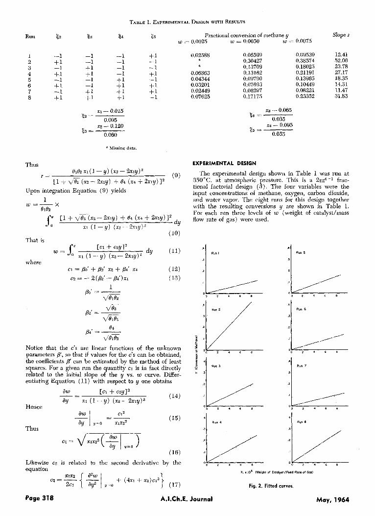
TABLE 1. EXPERIMENTAL DESIGN WITH RESULTS

t 5 Fractional conversion of methane y Slope s w = 0.0050 w = 0.0075

Run E2 53 E4 w = 0.0025

-1 +1 -1 i-1 -1 +I -1 +l

-1 -1 +l +I

+l +l

-1 -1

-1 -1 -1 -1 +1 +1 +I + I

XI - 0.015

0.005 x2 - 0.120

0.060

52 =

E3 =

* Missing data.

$.I -1 -1 +1 -1 + I f l -1

Thus

(9) e lezx l ( i -y ) ( ~ ~ - 2 2 x 1 y ) ~

r = [ 1 + VK ( ~ 2 - 2 x 1 ~ ) + ‘64 ( ~ 4 + 2 x 1 ~ ) Iz

Upon integration Equation (9) yields

w = - X 1

elez

dY (10)

9 [ 1 + vG&2 - 2x1y) + 84 (x4 + 2my) l2 JO x1 ( 1 - y ) ( X P -22?;1y).’

That is

dy (11) [Cl 4- c z y l ~

= f x1 ( 1 - y ) (xz- 2x1y)Z

Notice that the c’s are linear functions of the unknown parameters @’, so that if values for the c’s can be obtained, the coefficients 8’ can be estimated by the method of least squares. For a given run the quantity c1 is in fact directly related to the initial slope of the y vs. w curve. Differ- entiating Equation (11) with respect to y one obtains

(14) aw CCl + czy12

ay -=

x1 (1 - y) (xz - 2xly)2 Hence

Thus

J 8 -

Likewise cz is related to the second derivative by the equation

0.02588 #

#

0.06863 0.04344 0.03201 0.02449 0.07625

0.06599 0.30427 0.13709 0.13162 0.09790 0.07693 0.06297 0.17175

23 - 0.065 5 4 =

5 5 =

0.035

0.055 x4 - 0.095

0.09539 0.38574 0.18025 0.21191 0.13965 0.10449 0.08221 0.23352

12.41 52.06 23.78 27.17 18.35 14.31 11.47 31.83

EXPERIMENTAL DESIGN

The experimental design shown in Table 1 was run at 350°C. at atmospheric pressure. This is a 2111~-~ frac- tional factorial design ( 3 ) . The four variables were the input concentrations of methane, oxygen, carbon dioxide, and water vapor. The eight runs for this design together with the resulting conversions y are shown in Table 1. For each run three levels of w (weight of catalyst/mass flow rate of gas) were used.

.4 I Run 5

3

2

Page 318 A.1.Ch.E. Journal

:I;.,./ “;, 0 0 2 4 6 8

1 ------- 0

0 2 4 6 8

X, I lo’ (Weight of CalalyrtlFeed Rate of G o d

Fig. 2. Fitted curves.

May, 1964

Run

1 2 3 4 5 6 7 8

TAELE 2. SUMMAHY OF RESULTS FOR MODEL I

A c1’ = bo’ + ba’r2 + b4’m

bo‘ = -0.0007 bz’ = 0.027 _t0.0004* 20.002*

A CIP x 104 c 1 ~ x 104

20.54 13.93 47.98 58.08 16.70 25.27 64.32 53.56

24.27 14.35 52.62 59.69 14.55 23.45 60.68 50.75

$(GI#) x 104 = 1.72

b4‘ = 0.008 r0.002”

A ( ~ 1 ’ - cl’) x 104

4 . 7 3 -0.42 -4.64 -1.61 +2.15 + 1.82 +3.64 +2.81

* The numbers following ? signs are standard errors.

ANALYSIS OF DATA

The data which are plotted in Figure 2 can be iepre- sented to a good approximation by eight straight lines. Curvature is slight in this region, and higher values of w would be needed to show a marked departure from a linear relationship. The reaction however could not be controlled at higher values of w, and therefore no data could be obtained in this region.

The slopes of these eight straight lines were estimated by least squares and are given in Table 1. These calcula- tions as +ell as all others in this paper were performed with the experimentally recorded values of the variables x and w. These values differ slightly from those given in Table 1 because it was virtually impossible because of experimental error to set all the variables exactly at the desired levels.

Model 1.

The slope s estimates the derivative - 1 Mak- aw y=o

ing this replacement in Equation (16) one obtains

Using these CI’ values in Equation (12) one can obtain by least squares the results shown in Table 2.

The residual sum of squares 2 (c’ii - c ’ I ~ ) ~ is 67.319

x lo-*, and the corresponding mean square is 13.463 x with 5 deg. of freedom. The ratio of this mean

square to the estimated mean square error $(a’) [see Appendix] calculated from the fitted slopes si ( i = 1, 2,

, 8) is 4.53. The upper 5% point for the F distribu- tion with 5 and 14 deg. of freedom is only 2.96, which indicates that model I is inadequate since the value of the ratio considerably exceeds thi? value.

Of prime importance at this point is the unusual be-

havior of the residuals a’ - ci’ which provides a valuable clue as to what modification of the model might be tried next. Notice that the sign of the first four residuals is neg- ative and the sign of the last four is positive. As can be seen from Table 1 the signs of the residuals are perfectly correlated with the concentration of carbon dioxide. That is, model I does not take the concentration of carbon di- oxide properly into account. Recall that in accordance with model I the reaction yields nonadsorbed carbon di- oxide. So a logical modification would be to assume car- bon dioxide is adsorbed. To keep the model as simple as

8 A

i=l

A

possible further assume that water is not adsorbed. By doing this one ensures that the new model, model 11, con- tains three parameters 0 the same number as model I. Modrl I1

Following a similar development to that used in obtain- ing Equation (11) for model I one obtains for model I1

1 8152

X w = -

y [ l + V & ( x 2 - 2 x 1 y ) +03(x3+1C1y)l2 s, X l ( 1 - y ) (x2 - 2x1y)Z dY (19)

which can be rewritten as

where c1 = 8” + 82’’ X 2 + /33” 1 3

c2 = ( 8 3 ” - 2fl2”) 11

(21)

(22) Po” = = 1

\ /BIB2

The derivatives for model I1 yield results which are similar to those for model I:

aw If- I is replaced in Equation (23) by the quantity

ay y = o

s, a value for ci” can be calculated for each of the eight runs; that is

__-

(25) cl)# =

With these values Equation (21) can be fitted by least squares and the results analyzed. The summary of the results for model I1 is shown in Table 3.

TABLE 3. SUMMARY OF RESULTS FOR MODEL 11

A C l ” = bo” + b2”x2 + ba”a3

bo” = - 0.0003 b2” = 0.027 b4” =0.0063 r0.0006* r0.003” -t0.0058*

Run <

1 2 3 4 5 6 7 8

A x 104 ci” X 104

20.54 16.91 13.93 16.81 47.98 54.66 58.08 52.80 16.70 21.83 25.27 21.20 64.32 58.05 53.58 58.12

S(Cl”) x 104 = 1.72

A ( CI - G I ” ) X 104

+3.63 -2.88 -6.08 +5.28

+4.07 +6.27 -4.56

-5.13

0 The numbers following -C signs are standard errors.

Vol. 10, No. 3 A.1.Ch.E. Journal Page 319

n A TABLE 4. SUMMARY OF RESULTS FOR MODEL 111 The residual sum of squares S (cli” - c ~ i ’ ’ ) ~ is 197.06 X -

i = l and the corresponding mean square is 39.41 X

with 5 deg. freedom. The ratio of this mean square to the mean square error s2(ci”) is 13.27, which indicates that model I1 is also inadequate. Once again however by carefully examining the residuals one can gain valuable insight into the precise nature of the defects of this model. It will be noticed upon comparison with Table 1 that the signs of the residuals are now perfectly correlated with the concentration of water vapor.

Model I involved nonadsorbed carbon dioxide and ad- sorbed water, and model I1 involved adsorbed carbon dioxide and nonadsorbed water. Model I was shown to fail with regard to the manner in which carbon dioxide was taken into account, and model I1 was shown to be like- wise inadequate with respect to water. I t is apparently necessary to consider a model in which carbon dioxide and water are both adsorbed. In contrast to both models I and I1 which each involved three parameters, one will now be concerned with a more complex model containing four parameters,

Model 111

Starting with the assumptions that both carbon dioxide and water are adsorbed and following a derivation similar to those for models I and I1 one obtains for model 111

Run 1 2 3 4 5 6 7 8

cl~il x 103 15.57 11.94 25.99 31.53 13.56 18.52 34.03 29.87

A CP’ x 103 ( ~ 1

15.99 11.03 27.04 30.92 14.08 18.55 34.14 29.26

A - clq x 103

-0.42 +0.91 -1.05 +O.Sl -0.52 -0.03 -0.11 +0.61

S (c1q x 103 = 0.85 * The numbers following -C signs are standard errors.

The results of fitting Equation (28) by least squares are

shown in Table 4. The residual sum of squares 2 (cii’”

- c ~ i ’ ” ) ~ is 3.013 x and the residual mean square is 0.784 x 10-6 with 4 deg. of freedom. The ratio of this residual mean square to s2(c”’) [see Appendix] is 1.83, which indicates that the mode1 is adequate since F4,14(0.95) = 3.11. Also the residuals show no obvious

8

i = l A

~~ ~

dY (26) 1 + d K ( ~ z - 2 ~ 1 y ) + e 3 ( x 3 + “‘9) + 04(x4 + 2xl9)i3

x1( 1 - y ) (x2 - 2x1y)S

which can be rewritten as systematic pattern but seem to be random. Therefore model 111 appears to be adequate. Not only can one say

?I [Cl+ c2 y]3 ( 2 7 ) that the present mechanism offers a satisfactory explana- tion of the data, but also this is so when one has severely strained the model and carefully considered plausible al- ternatives. Thus the major objective of this paper is ac- complished. An appropriate form for a reaction rate equa- tion for the catalytic oxidation of methane has been found.

The analysis can now be carried a step further by determining estimates for the four parameters 8. Rough estimates can most easily be found by substituting b’s for the corresponding /3’s in Equations ( 3 0 ) , (31) , ( 3 2 ) , and ( 3 3 ) , and solving for the 8’s. The values so obtained can be used as initial guesses for the parameters in a non-

(31) linear Ieast-squares calculation (1, 2 ) to obtain better estimates. Incidentally one of the practical aspects which is of critical importance in using nonlinear estimation suc-

(32) cessfully is obtaining good first guesses for the parameters, and the approach outlined above provides such initial

(33) Residual sum

J x1( 1 - y) (x2 - 2x19) dY where

c1 = Po’” + PA’” x2 + 83’’’ x3 + p4”’ x*

C! = (2B4”‘ + 83“‘ - 2p2”’) XI

(28)

(29)

11, 1 (30) po =

9 8 i 0 2

dz- jya102

v8102

p2”’ == -- ps’” = 83

e4 values. The results were ,,, 8 4 =

of squares fY8102

A h A A 22 A The derivatives for model 111 differ from those of models el e2 83 84 S (yk-yk) ’ I and 11: k = l

By solving

By using (34) nonlinear

estimation 125,000 33,400 52.4 63.4 1.39 x lov5 Although there is fairly good agreement between the

(35) A corresponding 0 values, the residual sum of squares for nonlinear estimation is considerably smaller. The princi- pal reason for this fact is that in this treatment the authors have restricted themselves to the consideration of straight- line relationships between y and w for each run, whereas in fact not on1 is curvature to be expected, but also it can be detecte di from a closer statistical analysis. An exam- ination of the residuals from the fitted straight lines for

-- equations 118,000 30,300 58.7 63.1 3.18 x

(4x1 -k XZ) 3 c13 + c12c2

Ni (x1x22) 2

A value of cl”’ for each run can be calculated by replacing

”’ Equation (34) by the estimated ’lope ’;

that is

( 3 6 ) c1’” =

Page 320 A.1.Ch.E. Journal May, 1964

example reveals a negative value for seven out of the eight final residuals, that is y - sw for the highest value of w in each of the runs. Furthermore the ratio of s”(y) = 1.33 x [computed from the residuals from the straight lines (see Appendix)] to s2 = 1.41 x (based on four pairs of duplicate runs in previous work indicates lack of fit, the ratio being 94.3 as compared with F4,14(0.95) = 5.9. Consequently the second deriv- ative could have been estimated, and the corresponding cz values could have been calculated. An analysis similar to that applied to the c1 values could have been applied to the cz values. In some cases this procedure of using higher-order derivatives may be useful.

DISCUSSION

The main aim of thls paper has been to show how one can proceed in a sequential manner in a model building situation starting with a tentative model which has a theo- retical basis. The data are analyzed in the light of this particular model in such a way as to pinpoint precisely the inadequacies of this original conjecture. The model is modified in a IogicaI manner, and the data are then re- analyzed. Defects are once again revealed, and the model is modified further and so forth. One eventually arrives at an adequate model by using this iterative, diagnostic technique. The emphasis has been on an attempt to for- mulate a method for improving models, as opposed to a procedure for proving or disproving (that is, accepting or rejecting) them.

In any least-squares analysis of course it is possible to check the lack of fit by examining the residuals and in particular the residual sum of squares. As has been shown however residuals can be further analyzed in a way that is particularly meaningful. The object of the analysis is not especially to establish lack of fit but to provide some indication of the nature of this lack of fit to help the ex- perimenter in deciding how the model might be modified.

The technique has been illustrated by an example in which statistically designed experiments were employed. A number of questions arise. Could the method have been used if the experiments had not followed a factorial ar- rangement? The answer is yes, but in the example the implications of the residuals could not have been so readily interpreted. Nevertheless it would have been pos- sible to proceed exactly as before in fitting the linear relationship between ci and the x’s [for example, Equa- tion (12) for model I] provided only that the data points yielded at least as many such independent equations as there were coefficients to be estimated. The correlation between the residuals and the variables x however would probably not have been so obvious, although it could have been discovered either graphically by a plot of the resi- duals vs. x or by making the corresponding analytical calculation.

Fractional designs are usually employed for estimating coefficients similar to the $s above. However since ex- perimenters are primarily interested in the 8‘s and not the /3’s, should it not be possible to devise better designs for their purposes by focusing attention more directly on the problem of estimating the Bs? That is although the method is a valid one, as demonstrated by the kinetic ex- ample, could it not be made more efficient. This question is presently under investigation.

A number of other things must also be considered when designing an experiment in a model building situation. For instance in the example quoted above no fewer than eighty mechanisms were put forward as possible. It is of course well known that no mechanistic theory can be mathematically proved. I t can only be said that the ex- perimental data have failed to contradict a proposed

mechanism. It can happen however that a model or group of models is never really placed in jeopardy by a particu- lar set of experimental runs. That is to say the mechanism could be wrong in particular specific ways, and yet these discrepancies could not be revealed by the particular ex- periments performed. It is hoped that further work will be forthcoming on the specific problem of how best to plan experiments which will reveal and verify a particu- lar mechanism, that is which will discriminate among rival candidate models.

ACKNOWLEDGMENT

The authors are grateful to Professors G. E. P. Box and C. C. Watson for invaluable suggestions and constant encouragement in this investigation and also to the Wisconsin Alumni Re- search Foundation and the United States Navy through the Office of Naval Research under Contract Nonr-1202, Project NR 042 222, for financial support. The Kohler Foundation, which provided resident fellowshi s at the Kemper K. Knapp Memorial Graduate Center, helpelf to make this interdisciplin- ary work possible.

NOTATION

UCH4 = activity of methane acoZ = activity of carbon dioxide a H Z o = activity of water vapor aoz = activity of oxygen b = estimate of fl ci = true quantity defined for model I by Equation

(16), for model I1 by Equation (21), and for model I11 by Equation (28)

= true quantity defined for model I by Equation (17), for model I1 by Equation (22), and for model 111 by Equation (29)

CI’ = calculated value of ci defined by Equation (18) ci” = calculated value of ci defined by Equation (25) CI”’ = calculated value of ci defined by Equation (36) cz = total concentration of empty active sites Cz.z = concentration of adjacently located empty active

C H ~ O = total concentration of adsorbed water CH2O.HzO = concentration of adjacently adsorbed water C O ~ = total concentration of adsorbed oxygen CoZ.oz = concentration of adjacently adsorbed oxygen ki = sate constant kz = rate constant K = thermodynamic equilibrium constant of the

L = total concentration of active sites m n r = overall reaction rate r l = adsorption rate for oxygen r2 = rate of surface reaction r3 = desorption rate for water s S

s ( ) = standard deviation of ( ) 2( ) = variance of ( ) t = time of reaction w = (weight of catalyst)/(mass flow rate of gas) wij xi = mole fraction of methane xz x3 = mole fraction of carbon dioxide x4

y yu yij

c2

sites

methane oxidation reaction

= constant in Equation (3) = number of observations in a given run

= slope of fitted y vs. w curve = number of equidistant active centers adjacent to

each other

= the jth value of w in the ith run

= mole fraction of oxygen

= mole fraction of water vapor = fractional conversion of methane = the jth value of y in the ith run

= the least-squares estimate of zlij, namely siwij A

Vol. 10, No. 3 A.1.Ch.E. Journal Page 321

Greek Letters

fi = true parameter value [q] = concentration of chemical substance q at time t [?lo = initial concentration of 7 at time t = 0 0 = first-order rate constant 61 = overall reaction rate constant 82 = 63 =

04 = 85 = 66 = 67 =

5 = v =

adsorption equilibrium constant for oxygen adsorption equilibrium constant for carbon di- oxide adsorption equilibrium constant for water vapor equilibrium constant of surface reaction adsorption rate constant of oxygen surface reaction rate constant degrees of freedom standardized variable defined in Table 1

Superscripts A = estimated quantity ’ = model I “ = model I1 ”’ = model I11 Subscripts i i k

= run number (i = 1, 2, . . . , 8) = experiment number within a run (1, . . . , m) = experiment number (1, 2, . . . , 2 2 )

LITERATURE CITED 1. Booth, G. W., and T. 1. Peterson, I .B .M. Share Program Pa.

No. 687 WL NL 1. “Non-Linear Estimation” (1958). 2. Box, G. E. P., Ann. N. Y. Acad. Sci., 86, 792 (1960). 3. - , and J. S. Hunter, Technometrics, 3, 311 (1961). 4. - , and W. G. Hunter, ibid., 4, 301 (1962). 5. Faith, W. L., “Air Pollution Control,” Wiley, New York

6. Hougen, 0. A., and K. M. Watson, “Chemical Process Prin-

7. Mezaki, R., Ph.D. thesis, Univ. Wisconsin, Madison, Wis-

MnnuPcript received May 17 1983; revision received AuguH 14, 1963;

(1959).

ciples, Part 111,” Wiley, New York (1950).

consin ( 1963 ) . paper accepted August 16,1963.

APPENDIX: ERROR ANALYSIS

squares, that is After the eight slopes si have been determined by least

2 wijyij

j=1 si = ( i = 1,2, . . ., 8 ) 2 wij2

5=1

it is possible to obtain a pooled estimate s2(y) of the experi- mental error variance u2 from

A 2 (t j i j-- i j)2

- - iZ1 j=1 18.703 x 10-4 - - 14

s2(y) =

vi

t=1 1.3359 x 10-4

or s(y) = 1.156 x 10-2

Therefore a pooled estimate s2( s) of the variance of the slope is

f: visB(si)

i = l s2(s) =

v;

i=l

c vi i=l

1.3359 X IJ Y i

14 2 7 i=l c: wij2

j=1 1.3359

14 s Z ( S) = - 18.3217 = 1.7483

that is

To determine s( ci’) let us use the linear approximation S(S) = 1.3222

and

Thus 1 C‘li C’ l i

2 Si Si S(C’1i) = - . - * 1.3222 = 0.6611 -

from which one can obtain the pooled estimate 8

and

2 Y i i=l

For model I1 one obtains identical results; that is

s2( ~’’1) = ~ 2 ( C’I) = 2.9715 X

S(c’’1) = ~ ( c ‘ I ) = 1.7238 X

Analogously for model I11

and c’’’li = xlii/3 x2i si-113

1 C’”1i

Thus 1 d”1i C”‘1i

3 si Si 1.3222 = 0.4407 - s( C”’1i) = - -

from which one can obtain the pooled estimate

5 vis2(c”’li)

- i= l s2( c”‘1) = / 5 vi

and

A.1.Ch.E. Journal

t=i 6.0015 ?( 10-6

= 0.4287 X lod6 14

S(c’’’1) = 0.6548 X

Page 322 May, 1964