IntroductionThe Nif Dağı Research Project has been led by Prof. Dr. Elif Tül Tulunay since 2006. Nif Dağı (Mount Nif) is located at the eastern side of Izmir province, in Turkey’s western Anatolia region. The project is carried out in four differ-ent excavation sites, which are located in the southeast of Nif Dağı (Tulunay 2006). A significant site of the pro-ject is Karamattepe, defined as a rural metal production area in the Archaic Period (6th century BC), which stands apart because of its rich metal finds including approxi-mately 500 pieces of iron and bronze arrowheads, four metal production furnaces and extremely high amounts of slags. Given the rich metal finds, the area was probably used as a metal production workshop. No inclusive clas-sification study similar to early Neolithic El Khiam arrow-heads has been found for comparing the arrowheads produced in this region with those found in the anteced-ent or contemporaneous regions (Echegaray 1966:50). Although there is a significant lack of scholarly interest in metal finds dating from before the Persian invasion (5th century BC) in Western Anatolia, a common typology could be useful for the archaeologists working in the area to compare the production processes and to clarify social and economic relations of the period. When analysing the current status of the excavation area, one can see that since 2006, a total of 483 arrowheads made of iron and

bronze have been unearthed. In the excavation process, numerous academic publications related to arrowheads have been added to the literature. Associate Professor Dr. Daniş Baykan has also carried out a typological study in 2012 (Baykan 2012). In this study, arrowheads were clas-sified into nine different categories, with seven of them present in Karamattepe.

Baykan’s classification study only took into considera-tion the material (iron or bronze) and the observable simi-larities of the arrowheads, especially those of appearance; also, this research was limited to items from this particular excavation area.

Since 2017, all metric data obtained in the related excavation process have been digitalized. Nevertheless, many variations within 10 years of collected data and vari-ous omissions due to missing measurements have been detected in the data set.

The main objective of the current study is to create an unbiased classification tool which will cover both met-ric and categorical characteristics for present and future arrowheads gathered from Karamattepe, an outstand-ing region of West Anatolia for metal production in the Archaic period; as well as to resolve the lack of a common typological base by providing a comparison with similar –contemporaneous – arrowheads found in nearby regions. Of course, it would not be accurate to create a compre-hensive model to define all types of Archaic period arrow-heads from such a limited data set; however, the common metrics for the arrowheads are thought to be sufficient for a general assessment.

Tuncali Yaman, T. 2019. A Model-Based Statistical Classification Analysis for Karamattepe Arrowheads. Journal of Computer Applications in Archaeology, 2(1), pp. 12–20. DOI: https://doi.org/10.5334/jcaa.20

Beykent University, TRtutkutuncali@gmail.com

RESEARCH ARTICLE

A Model-Based Statistical Classification Analysis for Karamattepe ArrowheadsTutku Tuncali Yaman

The Nif Excavation Project is carried out by Elif Tül Tulunayin the southeastern part of Nif Dağı (Mount Nif) located in the eastern province of İzmir, Western Anatolia, Turkey. Since 2006, a total of 483 arrowheads made of iron and bronze have been found in Karamattepe, a territory with important sectors of rich metal finds, especially arrowheads. In the excavation process, Daniş Baykan implemented the first typological study related to arrowheads in 2012. The main objective of the current study is to create an unbiased classification tool which will cover both metric and categorical characteristics for present and future samples gathered from the same region; as well as to resolve the lack of a common typological base by providing a comparison with similar –contemporaneous– arrowheads found in nearby regions. For this purpose, Multinomial Logistic Regression was selected; and in order to provide a more coherent prediction, the Multiple Imputation (MI) Method was employed to complete the missing data. The study aims to develop the interpretation of archaeological data, while setting a unique example of the implication of the stated methods for the specified data.

Keywords: Arrowheads; Classification; Multiple Imputation

journal of computerapplications in archaeology

Tuncali Yaman: A Model-Based Statistical Classification Analysis for Karamattepe Arrowheads 13

Given this objective, the following sections include information about the data at hand, followed by informa-tion on the as yet missing parts of the data set and an over-all introduction of the data completion model selected in accordance with the lack of a reliable estimation model. Classification results of the Imputation Method will be discussed in light of the aim of the study, followed by sug-gestions for future methodologies.

Material and methodsMaterialThis section contains illustrative statistics pertaining to the arrowheads, excavated within a 10-year interval. Below is the distribution of a total of 483 arrowheads; 468 made of iron and 15 made of bronze, according to Baykan’s typology (Table 1).

The descriptive statistics calculated from the data at hand for all the metric variables of arrowheads are:

Weight (gr), Length (cm), Width (cm), Thickness (cm), Case Width (cm), Stem Width (cm), Driller Length (cm), Helve Thickness (cm), Material (bronze, iron), Absence (Yes, No) and Elevation (cm). They are shown in Table 2.

For the classification process, given the aim of the study, a Multinomial Logistic Regression Model (Hosmer & Lemeshow 2000) was run with the Stepwise method to include all the variables; however, the procedure could not be completed due to the missing elements in the data set. Therefore, a few variables with the highest amount of incompleteness such as Stem Width (cm), Driller Length (cm), and Helve Thickness (cm) were omitted and the model was run again, resulting only in a useless estimate which gave statistically insignificant results without taking any of the variables into consideration.

Hence, in order to establish a reliable model that fits our research purpose, the missing data must be com-pleted first. Due to the physical inaccessibility of the exca-vated material that is currently stored in local museum depots, a data completion methodology was adopted using a suitable data imputation method. In the follow-ing section, first the theoretical information about the applied methods will be detailed followed by the results obtained by the application.

Methodology This section discusses the missing data problem in sta-tistics and categorization models, as well as the Multiple Imputation (MI) Method and cases from literature.

The Missing Data ProblemThe problem of missing variables in a data set can be found in almost all empirical research (Little & Rubin 2002). The question: “if the data were complete, would the results of the research be different?” (Gold & Bentler 2000; Sung & Geyer 2007) unfortunately does not – and will not – have a

Table 1: Distribution of arrowheads according to the typology developed by Baykan (2012).

Typology Frequency %

Type 1 289 59.8

Type 2 129 26.7

Type 3 28 5.8

Type 4 13 2.7

Type 5 8 1.7

Type 6 5 1

Type 7 2 0.4

N/A 9 1.9

Total 483 100

Table 2: Descriptive statistics of the arrowheads.

Total Type

Type 1 Type 2 Type 3 Type 4 Type 5 Type 6 Type 7 N/A

Mean n Mean n Mean n Mean n Mean n Mean n Mean n Mean n Mean n

Weight 8.92 456 8.05 274 11.87 123 5.08 28 8.70 12 4.38 6 4.43 2 10.68 2 11.12 9

Length 5.67 471 5.79 286 5.59 123 5.74 28 5.62 13 3.56 8 3.75 4 4.40 2 5.99 7

Width 1.05 324 1.02 268 1.15 24 1.37 3 0.96 12 1.24 7 0.97 3 1.50 1 1.57 6

Thickness 0.80 220 0.80 128 0.94 57 0.45 18 0.77 3 0.66 6 0.40 1 0.85 2 0.66 5

Case width 1.13 110 0 1.16 102 0 0 0.70 4 .070 3 0 1.2 1

Helve thickness 0.55 295 0.55 248 1.34 5 0.40 24 0.50 12 0.80 1 0 0.30 1 0.75 4

Stem width 1.43 28 0.90 1 0 1.44 25 0 1.30 1 0 1.70 1 0

Driller length 3.65 425 4.12 261 2.59 116 4.52 26 2.57 12 2.50 4 2.35 2 4.40 1 2.73 3

Elevation 437.2 419 436.9 257 437.5 110 439.4 23 435.6 8 436.9 8 434.9 3 437 2 438.1 8

Abs Yes 103 46 38 3 7 5 0 2

No 338 225 77 20 4 3 2 6

Material Iron 468 289 129 28 13 0 0 8

Bronze 15 0 0 0 0 8 2 1

Tuncali Yaman: A Model-Based Statistical Classification Analysis for Karamattepe Arrowheads14

specific answer, since incompleteness causes a decrease in the performance of parameter estimation and sensitivity of the method. If the missing data pattern is non- random, the concern about bias will be added throughout the course of the research. In this context, bias results in the failure of observed data to represent the incomplete parts (Gold & Bentler 2000). In recent years, there has been a growing interest towards discussing missing data mecha-nisms and consequently different techniques have been introduced (Enders 2003).

The Missing Data Problem in Classification StudiesThe incomplete data problem may either evolve naturally, or deliberately. The data set may include latent variables due to the design of the researcher or deviation of respond-ents (Rubin 1991). For instance, any missing content within a data set based on examinations or tests – which would serve to the identification of a specific illness or the categorization of related patients – would create an error in the decision-making process. As omissions increase the complexity of the analysis, numerous studies have been conducted to analyse the missing data patterns and evaluate their effects on the results of regression models. Incompleteness patterns are primarily categorized into two types: missing at random and missing at non-random. The non-random pattern may cause an additional effect of bias, since the missing data cannot be assumed to be simi-lar to the unobserved parts of the data. Hence, it is more complicated to handle (Gold & Bentler 2000).

Handling The Missing Data ProblemIn the scientific literature, missing data is addressed in var-ious ways; the first one is to omit the missing components and only treat the observed ones (Soley-Bori 2013) While facilitating the implementation, this method excludes the information of incomplete cases. Thus, with the possible differences between the missing and/or observed parts being omitted, the results may fail to reflect the character-istics of the whole data set.

Another approach assigns a predicted value for each missing item in a data set, using the means of observed components to replace the missing values. This algorithm is called Single Imputation and applies standard statistical procedures to a newly predicted complete dataset. Since single imputation considers the process as if there is no missing value in the dataset, it cannot reject the uncer-tainty of predictions; hence it might yield a biased result-ing variance of estimated variables which tend to converge to zero (Yuan 2010).

Rubin (1987) thus introduced the concept of multiple imputation, which is a part of the Markov Chain Monte Carlo methods, where all possible values for the latent variables are evaluated, and each one of them is used in parameter estimation (Gold & Bentler 2000; Yuan 2010; Rubin 1991). Markov Chain Monte Carle (MCMC) methods are mostly used in applications where there are intractable densities which are approximated by a finite number of samples (Gelman et al. 2014). The MI procedure imputes each missing variable with a set of possible values. Among the variety of these offered values, the uncertainty of

missing variables can be represented. The algorithm could thus perform the standard data analysis procedure to each completed dataset. Then it combines and compares the results for the inference.

In the following section, after a short description about MCMC to clarify the context, more detailed information about MI will be given. For more background about these methods in the literature, see Horton & Lipsitz (2001), Enders (2010), Raghunathan et al. (2001), and Brand et al.(2003).

Markov Chain Monte Carlo Methods (MCMC)A Markov chain with a stationary distribution π, is a sequence of random variables in which the distribution of each element depends on the value of the previous one. In MCMC, one constructs a Markov chain long enough for the distribution of the elements to stabilize to a com-mon distribution. This stationary distribution is the distri-bution of interest. By repeatedly simulating steps of the chain, it simulates draws from the distribution of interest (Molenberghs & Kenward 2007:113). For a detailed discus-sion of this method see Shafer (1997).

In Bayesian inference, information about unknown parameters is expressed in the form of a posterior prob-ability distribution. That is, through MCMC, one can simu-late the entire joint posterior distribution of the unknown quantities and obtain simulation-based estimates of pos-terior parameters that are of interest. (O’Hara et al. 2002; Acquah 2013).

Suppose that we have a m × n matrix X, that consists of observed and missing variables, such that X = (Xobs, Xmis) its corresponding n-dimensional parameter vector for the given model is θ = (θ1, θ2, …, θn)

T, and the m- dimensional output vector of the model is Y = (Y1, Y2, …, Ym)T. Using the Bayesian idea we can write the conditional probability of Xmis:

, , , ,1

( , ) ( , | ( , , , )

( ) ( , ) ( ,

,

)

)

,| |

mis mis obs mis obs

m

mis i obs i i mis i obs ii

X p X X p x x Y

p p x x p y x x

Yπ θ θ α θ

θ θ θ θ=

=

= ∏where we assume X is independent of θ, i.e.

( ) ( ) ( ), , , ,, | ,mis i obs i mis i obs i ip x x p x x p xθ = =

( ) ( ), ,| , , |i mis i obs i i ip y x x p y xθ θ =

The procedure starts with Bayesian learning for variables, and then an MCMC technique is employed to draw sam-ples from the probability distributions learned by the Bayesian network. The algorithm continues iteratively, until convergence is reached. This method provides unbi-ased estimates, as well as the confidence levels of the imputation results (Ni & Leonard II 2005).

Multiple Imputation (MI)MI is a MCMC-based method for the analysis of incom-plete data sets. The main assumption of the method derives from the assumption that missing observations show a random distribution. A statistical analysis using

Tuncali Yaman: A Model-Based Statistical Classification Analysis for Karamattepe Arrowheads 15

multiple imputation method typically includes three main steps. The first step involves specifying and generat-ing plausible synthetic data values, called imputations, for the missing values in the data. The second step consists of analysing each imputed data set by a statistical method that will estimate the quantities of scientific interest. The third step pools the m estimates into one estimate, thereby combining the variation within and across the m imputed data sets (van Buuren 2007).

According to the notation of the procedure, Yj indicates that one of k incomplete random variables (j = 1, …, k) and (Y = Y1, …, Yk).

obsiY and mis

iY are denotations of the observed and missing parts of Yj. Jointly, observed and missing data in Y showed as ( )1 , ,obs obs obs

kY Y Y= … and ( )1 , ,mis mis mis

kY Y Y= … . Imputation of miskY is based on the

relation between the missing variable Yk and the k−1 predictors Y–j = (Y1, …, Yj–1, Yj+1, …,Yk), where the nature of the relation is primarily estimated from the units contributing to obs

jY . Joint modeling (JM) and fully conditional specifi-cation (FCS) have appeared as two recent approaches for multiple imputations.

Joint modelling starts its procedure by determining a parametric multivariate density p(y|θ) for Y with given model parameters θ. The posterior predictive distribu-tion of p(ymis|Yobs) and the appropriate prior distributions of θ are generated by a Bayesian framework under the assumption of an ignorable missing data mechanism (Rubin 1987). Unlike JM, fully conditional specification does not start with prominent multivariate density. In FCS a separate conditional density p(yj|Yj–1, θj) for each Yj–1 is implicitly defined by p(y|θ). In order to impute mis

jY given Yj–1, mentioned density is used. Performing multi-ple imputations by using FCS, all conditionally specified imputation models (such as linear regression for continu-ous variables, logistic regression for binary variables, and multinomial regression for polytomous variables) are iter-ated and each of them consists of one cycle through all Yj. According to Brand et al. (2003) the advantages of the method are listed as:

• Simple and versatile• Attributes close to the data, omits impossible data• Subset collection of predictors• Modular, can conserve costly work• Successful, both in simulations and execution

The simplicity of the method resulted in its applicabil-ity by several software programs. FCS application can be executed by the mice, transcan, mi, VIM, baboon packages in R, the multiple imputation command in SPSS and by the ice and multiple imputation command in SAS IVEware and STATA.

Before the data imputation procedure, the missing data distribution within all the variables (Weight (gr), Length (cm), Width (cm), Thickness (cm), Case Width (cm), Stem Width (cm), Driller Length (cm), Helve Thickness (cm) and Elevation (cm)) of the arrowhead data set has been examined. The “Missing Data Patterns” graph lists distinct missing data patterns. It shows that the data set does not have a monotone missing pattern which means that the

distribution of absence does not depend on the data. To be more specific, in this study, the missing data in the studied variables was not originating from (a) specific arrowhead(s) (see Figure 1). Given the missing data pat-terns and the diversity of variables in the imputation of the data set, the MI Method has been applied with the FCS procedure for this study, because this model com-pletes each and every variable with a characteristic regres-sion model and it gives stable results in case the missing data does not follow a specific pattern. In the imputation process of the missing data, different regression mod-els were established for each variable. Variables of the regression models are Weight (gr), Length (cm), Width (cm), Thickness (cm), Case Width (cm), Stem Width (cm), Driller Length (cm), Helve Thickness (cm) and Elevation (cm).

Detailed information and comparison regarding vari-ous data imputation methods can be found in Demirtas, Freels & Yucel (2008); van Buuren et al. (2006); Lee & Carlin (2010); and Yu, Burton & Rivero-Arias (2007).

The following section describes the results from the selected data completion model MI and the classification study.

ResultsBased on the FCS based MI results, the most suitable model was selected from 5 different imputation models. The selection criterion was set to be the minimum dif-ference between average and standard deviation values of missing and completed datasets. Table 3 shows the results for the arrowhead dataset variables in detail. The MI was performed in IBM SPSS 24 with the following com-mand:

DATASET DECLARE iteration.MULTIPLE IMPUTATION WEIGHT LENGTH WIDTH THICKNESS CASEWIDTH HELVETHICK STEMWIDTH DRILLERLEN ELEVATION/ANALYSISWEIGHT TYPE /IMPUTE METHOD=FCS MAXITER= 10 NIMPUTATIONS=5 SCALEMODEL=LINEAR INTERACTIONS=NONE SINGULAR=1E-012 MAXPCTMISSING=NONE/MISSINGSUMMARIES NONE /IMPUTATIONSUMMARIES MODELS DESCRIPTIVES /OUTFILE IMPUTATIONS=Imputation FCSITERATIONS=iteration.

10 Iterations have been executed in the procedure, and the existing typology classification (Baykan 2012) was set as Analysis Weight. Analysis Weight specifies a variable including analysis (regression) weights. The procedure consolidates analysis weights in regression and classifi-cation models used to assign missing values (IBM 2018).

The descriptive statistics obtained as a result of the procedure are presented below in comparison with the original data. Measured metric variables of arrowheads are Weight (gr), Length (cm), Width (cm), Thickness (cm), Case Width (cm), Stem Width (cm), Driller Length (cm),

Tuncali Yaman: A Model-Based Statistical Classification Analysis for Karamattepe Arrowheads16

Helve Thickness (cm), Material (bronze, iron), Plan Square (a location code in excavation area), Absence (Yes, No) and Elevation (cm).

After data completion, Multinomial Logistic Regression Analysis (Multinomial-LOGIT) was again carried out to determine the extent to which the arrowheads coincide with the given estimates and types determined accord-ing to the existing typology. Prior to the analysis, the first three categories of the type determined by this expert-based typology were preserved; while the other types (from Type 4 to Type 7) with low frequency were combined

to form a single group called Other. Multinomial-LOGIT was performed in IBM SPSS 24 with the NOMREG com-mand. The interactions between Weight and Length attributes (Weight*Length) were taken as an essential variable for the regression model, due to their high cor-relation coefficient (ρ = 0.493, p < 0.01). The other vari-ables were selected by Stepwise Forward Entry method (Le 1998:112) by considering their statistical significance. The interactive variable of weight and length (WEIGHT * LENGTH), MATERIAL, DRILLER LENGTH, and Absence (ABS) and (ELEVATION) variables have been chosen

Figure 1: Distribution of missing values.

Table 3: Descriptive statistics before and after data completion.

Original Data Missing Data Completed Data (N:483)

N Mean Standard Deviation

Frequency % Mean Standard Deviation

Weight 456 8.91 3.82 27 6 8.92 3.86

Length 471 5.67 1.30 12 2 5.67 1.30

Width 324 1.04 1.19 159 33 1.16 1.20

Thickness 220 0.80 0.24 263 54 0.78 0.33

Case Width 110 1.12 0.25 373 77 1.00 0.31

Helve Thickness 295 0.55 0.75 188 39 0.60 0.72

Stem Width 28 1.42 0.18 455 94 1.51 0.29

Driller Length 425 3.64 1.03 58 12 3.62 1.05

Elevation 419 437.20 3.32 64 13 437.22 3.38

Tuncali Yaman: A Model-Based Statistical Classification Analysis for Karamattepe Arrowheads 17

according to high statistical significance. Before evaluat-ing the parameter estimates of the model, it is essential check the overall effectiveness and the predictive power. The goodness of fit coefficient (–2 log λ) was found to be 876.815 for the ideal model (which has only a fixed term) and 417.427 for the restricted model (predicted with selected variables). The test statistic, used to test good-ness of fit under the hypothesis of validity of the ideal model is calculated below:

( ) ( )2 ( 2 log ( 2 log 459.388ideal rest

G λ λΔ = − − − =2(0,05;15)df :15, 24.99χ =

According to the Chi-Square Test, the null hypothesis is rejected (α = 0.05). The generated model is sufficient for prediction (Wilks 1938: 62). In the logistic regression analysis, the determination coefficient R2 gives misleading results. Thus, weighted Cox-Snell’s Pseudo R2 and Nagel-kerke’s R2 are preferred. According to Nagelkerke R2, the independent variables in the model explain 0.75 of the dependent variable (Table 4).

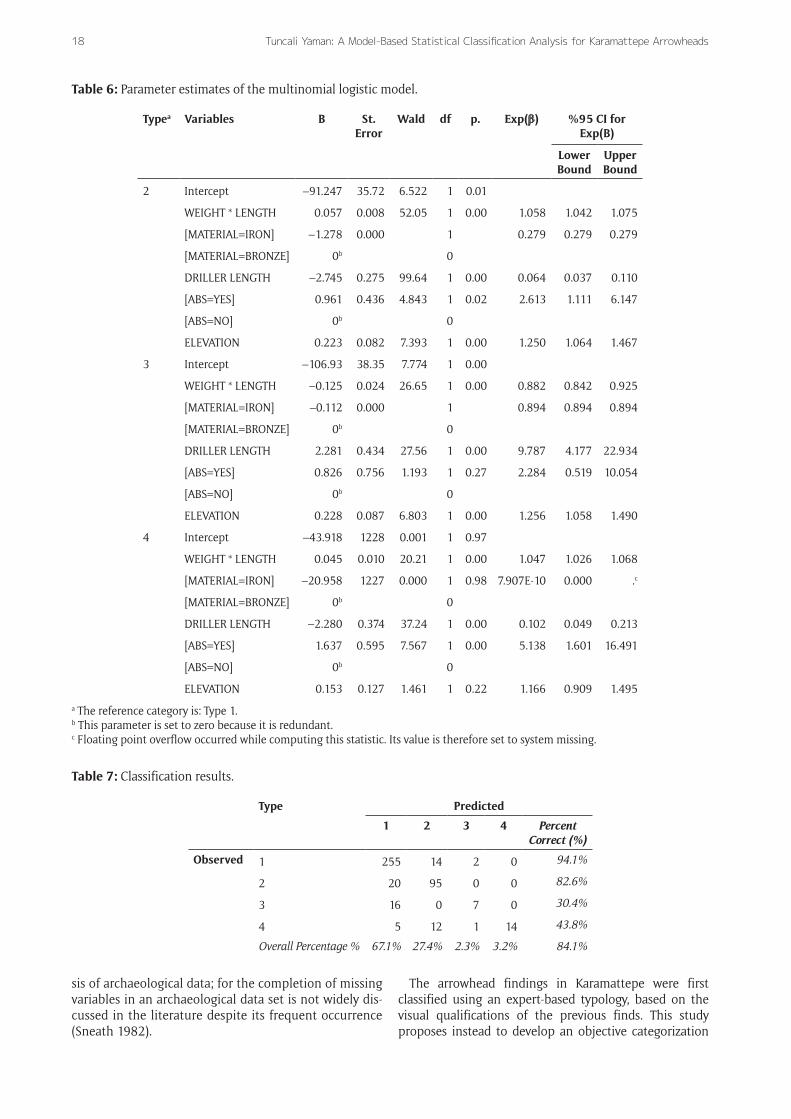
Since the large Chi-square values are taken as an indica-tion of the model’s predictive power and adequacy, predic-tion of the generated unrestricted model is found to be effective here (Sullivan, Ferguson & Donndelinger 2011). The parameter estimates obtained from the Multi-Nomial Logistic Regression Model and the measures of the good-ness of fit are detailed in the following tables (Tables 5 and 6).

When the compliance measures and likelihood ratio tests are examined in the context described above, it can be seen that all variables are statistically significant in the model.

In order to estimate the Multi-Nomial Logistic Regression Model, the category that has the highest frequency is determined as the reference category. Here, Type 1 is selected as the reference category and in the esti-mation results, For each type, the regression coefficient is interpreted as how that category compares to the refer-ence category (Kuhfeld, Tobias & Garratt 1994).

Interpretation of the coefficients in the logistic model does not make sense, and variables with values less than 1 odds ratio (indicated as Exp (β) on the Table 5) are inter-preted as variables that have significant influence on the change of the dependent variable and vice versa (Agresti 2002).

In the parameter estimates of the model, it is appar-ent that the ABS variable for Type 3 and MATERIAL and ELEVATION for Other have insignificant Wald test statistics due to the insufficient sample size. Fortunately, this does not affect the overall fit of the model. The overall correct assignment rate of the predicted model is 84.1% (Table 7).

Finally, it can be reported that the percentage of correct assignment of the model is relatively high. Correct assign-ment ratios obtained for Type 1 and 2 are higher than for Type 3 and Other because of the lower sample size of the latter.

Summary, discussion and future researchThis study first and foremost aims to create a proper clas-sification based on the high number of arrowheads from Karamattepe, With the clear lack of scholarly interest in the metal finds of the area (Baykan 2015), the absence of a common typology makes it harder for the archae-ologists working in the area to compare the production processes and to clarify social and economic relations of the period. This lack of common typology has formed the impetus for this study. The results are expected to facilitate any research and studies about Archaic arrow-heads in the region. On the other hand, this study also aims to present an example to the researchers working with similar cases of the use of technology for the analy-

Table 4: Goodness-of-fit criteria.

Criteria Value

AIC (ideal) 882.815

AIC (restricted) 453.427

Cox and Snell’s Pseudo R2 0.647

Nagelkerke R2 0.750

McFadden 0.524

Pearson Chi – Squared 11443.137

Relative Chi – Squared 417.427

Table 5: Measures of good compliance with the multi-territorial logistic regression model.

GoF (Restricted Model) Likelihood Ratio Test

AIC BIC –2logλ χ2 df p

Intercept 453.427 527.030 417.427a 0.000 0

WEIGHT * LENGTH 581.545 642.881 551.545b 134.118 3 0.000

MATERIAL 518.147 579.482 488.147 70.719 3 0.000

DRILLER LENGTH 744.169 805.504 714.169b 296.742 3 0.000

ABS 456.826 518.162 426.826b 9.399 3 0.024

ELEVATION 461.745 523.081 431.745b 14.318 3 0.003

a This reduced model is equivalent to the final model because omitting the effect does not increase the degrees of freedom.b Unexpected singularities in the Hessian matrix are encountered. This indicates that either some predictor variables should be

excluded or some categories should be merged.

Tuncali Yaman: A Model-Based Statistical Classification Analysis for Karamattepe Arrowheads18

sis of archaeological data; for the completion of missing variables in an archaeological data set is not widely dis-cussed in the literature despite its frequent occurrence (Sneath 1982).

The arrowhead findings in Karamattepe were first classified using an expert-based typology, based on the visual qualifications of the previous finds. This study proposes instead to develop an objective categorization

Table 6: Parameter estimates of the multinomial logistic model.

Typea Variables B St. Error

Wald df p. Exp(β) %95 CI for Exp(B)

Lower Bound

Upper Bound

2 Intercept –91.247 35.72 6.522 1 0.01

WEIGHT * LENGTH 0.057 0.008 52.05 1 0.00 1.058 1.042 1.075

[MATERIAL=IRON] –1.278 0.000 1 0.279 0.279 0.279

[MATERIAL=BRONZE] 0b 0

DRILLER LENGTH –2.745 0.275 99.64 1 0.00 0.064 0.037 0.110

[ABS=YES] 0.961 0.436 4.843 1 0.02 2.613 1.111 6.147

[ABS=NO] 0b 0

ELEVATION 0.223 0.082 7.393 1 0.00 1.250 1.064 1.467

3 Intercept –106.93 38.35 7.774 1 0.00

WEIGHT * LENGTH –0.125 0.024 26.65 1 0.00 0.882 0.842 0.925

[MATERIAL=IRON] –0.112 0.000 1 0.894 0.894 0.894

[MATERIAL=BRONZE] 0b 0

DRILLER LENGTH 2.281 0.434 27.56 1 0.00 9.787 4.177 22.934

[ABS=YES] 0.826 0.756 1.193 1 0.27 2.284 0.519 10.054

[ABS=NO] 0b 0

ELEVATION 0.228 0.087 6.803 1 0.00 1.256 1.058 1.490

4 Intercept –43.918 1228 0.001 1 0.97

WEIGHT * LENGTH 0.045 0.010 20.21 1 0.00 1.047 1.026 1.068

[MATERIAL=IRON] –20.958 1227 0.000 1 0.98 7.907E-10 0.000 .c

[MATERIAL=BRONZE] 0b 0

DRILLER LENGTH –2.280 0.374 37.24 1 0.00 0.102 0.049 0.213

[ABS=YES] 1.637 0.595 7.567 1 0.00 5.138 1.601 16.491

[ABS=NO] 0b 0

ELEVATION 0.153 0.127 1.461 1 0.22 1.166 0.909 1.495

a The reference category is: Type 1.b This parameter is set to zero because it is redundant.c Floating point overflow occurred while computing this statistic. Its value is therefore set to system missing.

Table 7: Classification results.

Type Predicted

1 2 3 4 Percent Correct (%)

Observed 1 255 14 2 0 94.1%

2 20 95 0 0 82.6%

3 16 0 7 0 30.4%

4 5 12 1 14 43.8%

Overall Percentage % 67.1% 27.4% 2.3% 3.2% 84.1%

Tuncali Yaman: A Model-Based Statistical Classification Analysis for Karamattepe Arrowheads 19

tool to include the metric and categorical qualifications of these arrowheads. For the classification method, the Multinomial Logistic Regression has been employed, used in conjunction with the Multiple Imputation (MI) FCS method to complete the missing data in order to provide a more coherent estimate. Analysis of all the indicators shows that the model is statistically coherent. In addition to that, the accordance of the results from the model with the expert-based typology is considered as an important factor for its coherence. The results are approximately 84% in accordance with the expert-based typology.

As stated above, the data set at hand has several quali-tative and regional limitations. Any common typology depicting an overall picture of archaic arrowheads in this region should be considered imprecise. However, if com-mon metrics could be provided for the arrowhead find-ings in the neighbouring regions, the model could be considered as a guiding model for a general description.

Hopefully, this study will be considered as the first step to determine a comprehensive typology of the Archaic arrowheads of Western Anatolia. In order to create a more inclusive typological model for future studies, it is essen-tial that data from a wider area within the region should be collected; while the imputation and categorization techniques are also updated with this newly acquired data. Future studies with wider extents are expected to contrib-ute to the sociological, economic and technological analy-sis in archaeological researches in Western Anatolia.

AcknowledgementsI am grateful to the site director, Prof. Dr. Elif Tül Tulunay and her deputies Assoc. Prof. Dr. Daniş Baykan and Assoc. Prof. Dr. Müjde Peker for their support.

Competing InterestsThe author has no competing interests to declare.

ReferencesAcquah, HD-G. 2013. Bayesian logistic regression

modelling via Markov Chain Monte Carlo Algorithm. Journal of Social and Development Sciences, 4(4): 193–197.

Agresti, A. 2002. Categorical data analysis. New York: Wiley Interscience. DOI: https://doi.org/10.1002/0471249688

Baykan, D. 2012. Nif (Olympos) Dağı kazısı metal buluntularının tipolojik ve analojik değerlendirmesi. In: Dönmez, H and Keskin, Ç (eds.), 27. Arkeometri Sonuçları Toplantısı, 23–28 May 2011, 154: 231–246. Malatya: Kültür Varlıkları ve Müzeler Genel Müdürlüğü Yayın.

Baykan, D. 2015. Metal finds from Nif-Olympus. In: Laflı, E and Patacı, S (eds.), Recent studies on the archaeology of Anatolia, 41–48. Oxford: Archaeopress.

Brand, JPL, van Buuren, S, Groothuis-Oudshoorn, CGM and Gelsema, ES. 2003. A toolkit in SAS for the evaluation of multiple imputation methods. Statistica Neerlandica, 57(1): 36–45. DOI: https://doi.org/10.1111/1467-9574.00219

Demirtas, H, Freels, SA and Yucel, RM. 2008. Plausibility of multivariate normality assumption when multi-ply imputing non-Gaussian continuous outcomes: A simulation assessment. Journal of Statistical Computation and Simulation, 78(1): 69–84. DOI: https://doi.org/10.1080/10629360600903866

Echegaray, JG. 1966 Excavaciones en la terraza de “El Khiam” (Jordania). Madrid: Bibliotheca Praehistorica Hispana.

Enders, CK. 2003. Using the Expectation Maximiza-tion Algorithm to estimate coefficient alpha for scales with item-level missing data. Psychol Methods, 8(3): 322–37. DOI: https://doi.org/10.1037/1082-989X.8.3.322

Enders, CK. 2010. Applied missing data analysis. New York: The Guilford Press.

Gelman, A, Carlin, JB, Stern, HS, Dunson, DB, Vehtari, A and Rubin, DB. 2014. Bayesian data analysis. Boca Raton: CRC Press.

Gold, MS and Bentler, PM. 2000. Treatments of missing data: a Monte Carlo comparison of RBHDI, Iterative Stochastic Regression Imputation, and Expecta-tion-Maximization. Structural Equation Modeling: A Multidisciplinary Journal, 7(3): 319–355. DOI: https://doi.org/10.1207/S15328007SEM0703_1

Horton, NJ and Lipsitz, SR. 2001. Multiple imputa-tion in practice: comparison of software packages for regression models with missing variables. The American Statistician, 55(3): 244–254. DOI: https://doi.org/10.1198/000313001317098266

Hosmer, DW and Lemeshow, S. 2000. Applied logistic regression. New York: John Wiley & Sons. DOI: https://doi.org/10.1002/0471722146

IBM. 2018. Multiple imputation. Available at: https://www.ibm.com/support/knowledgecenter/en/SSLVMB_24.0.0/spss/mva/syn_multiple_imputa-tion.html [Last accessed 23 December 2018].

Kuhfeld, WF, Tobias, RD and Garratt, M. 1994. Efficient experimental design with marketing research applications. Journal of Marketing Research, 31(4): 545–557. DOI: https://doi.org/10.2307/3151882

Le, CT. 1998. Applied categorical data analysis. New York: Wiley Interscience.

Lee, KJ and Carlin, JB. 2010. Multiple imputation for missing data: fully conditional specification versus multivariate normal imputation. American Journal of Epidemiology, 171(5): 624–632. DOI: https://doi.org/10.1093/aje/kwp425

Little, R and Rubin, D. 2002. Statistical analysis with missing data. New Jersey: Wiley. DOI: https://doi.org/10.1002/9781119013563

Molenberghs, G and Kenward, M. 2007. Missing Data in Clinical Studies. London: John Wiley & Sons. DOI: https://doi.org/10.1002/9780470510445

Ni, D and Leonard II, JD. 2005. Markov Chain Monte Carlo multiple imputation using Bayesian networks for incomplete intelligent transpor-tation systems data. Transportation Research Record, 1935(1): 57–67. DOI: https://doi.org/10.1177/0361198105193500107

Tuncali Yaman: A Model-Based Statistical Classification Analysis for Karamattepe Arrowheads20

O’Hara, RB, Arjas, E, Toivonen, H and Hanski, I. 2002. Bayesian analysis of metapopulation data. Ecology, 83(9): 2408–2415. DOI: https://doi.org/10.2307/3071802

Raghunathan, TE, Lepkowski, JM, van Hoewyk, J and Solenberger, P. 2001. A multivariate technique for multiply imputing missing values using a sequence of regression models. Survey Methodology, 27(1): 85–95.

Rubin, DB. 1987. Multiple imputation for nonresponse in surveys. New York: Wiley Classics. DOI: https://doi.org/10.1002/9780470316696

Rubin, DB. 1991. EM and beyond. Psychometrica, 56: 241. DOI: https://doi.org/10.1007/BF02294461

Shafer, JL. 1997. Analysis of Incomplete Multivariate Data. New York: Chapman & Hall/CRC. DOI: https://doi.org/10.1201/9781439821862

Sneath, PHA. 1982. Classification and identification with incomplete data. In: Laflin, S (ed.), Computer Appli-cations in Archaeology 1982. Conference Proceedings, 182–187. Birmingham: Centre for Computing and Computer Science, University of Birmingham.

Soley-Bori, M. 2013. Dealing with missing data: Key assumptions and methods for applied analysis. Boston: Boston University School of Public Health. Avail-able at: https://www.bu.edu/sph/files/2014/05/Marina-tech-report.pdf [Last accessed 23 December 2018].

Sullivan, E, Ferguson, S and Donndelinger, J. 2011. Exploring differences in preference heterogene-ity representation and their influence in product family design. In: ASME 2011 International Design Engineering Technical Conferences and Computers

and Information in Engineering Conference. Volume 5: 37th Design Automation Conference, 81–92. Parts A and B, Washington, DC, USA, August 28–31, 2011. DOI: https://doi.org/10.1115/DETC2011-48596

Sung, YJ and Geyer, CJ. 2007. Monte Carlo likelihood inference for missing data models. The Annals of Statistics, 35(3): 990–1011. DOI: https://doi.org/10.1214/009053606000001389

Tulunay, ET. 2006. Nif (Olympos) dağı araştırma projesi: 2004 yılı yüzey araştırması. AST, 23(2): 189–200.

van Buuren, S. 2007. Multiple of discrete and continuous data by fully conditional specification. Statistical Methods in Medical Research, 16(3): 219–242. DOI: https://doi.org/10.1177/0962280206074463

van Buuren, S, Brand, JP, Groothuis- Oudshoorn, CG and Rubin, DB. 2006. Fully conditional specification in multivariate imputation. Journal of Statistical Computation and Simulation, 76(12): 1049–1064. DOI: https://doi.org/10.1080/10629360600810434

Wilks, SS. 1938. The large-sample distribution of the like-lihood ratio for testing composite hypotheses. The Annals of Mathematical Statistics, 9: 60–62. DOI: https://doi.org/10.1214/aoms/1177732360

Yu, LM, Burton, A and Rivero-Arias, O. 2007. Evaluation of software for multiple of semi-continuous data. Statistical Methods in Medical Research, 16(3): 243–258. DOI: https://doi.org/10.1177/0962280206074464

Yuan, YC. 2010. Multiple imputation for missing data: Concepts and new development (Version 9.0). Rockville: SAS Institute Inc.

How to cite this article: Tuncali Yaman, T. 2019. A Model-Based Statistical Classification Analysis for Karamattepe Arrowheads. Journal of Computer Applications in Archaeology, 2(1), pp. 12–20. DOI: https://doi.org/10.5334/jcaa.20

Submitted: 04 November 2018 Accepted: 25 January 2019 Published: 04 March 2019

Copyright: © 2019 The Author(s). This is an open-access article distributed under the terms of the Creative Commons Attribution 4.0 International License (CC-BY 4.0), which permits unrestricted use, distribution, and reproduction in any medium, provided the original author and source are credited. See http://creativecommons.org/licenses/by/4.0/.

OPEN ACCESS Journal of Computer Applications in Archaeology, is a peer-reviewed open access journal published by Ubiquity Press.