ww.sciencedirect.com

b i om a s s a n d b i o e n e r g y 6 7 ( 2 0 1 4 ) 8e2 3

Available online at w

ScienceDirect

ht tp: / /www.elsevier .com/locate/biombioe

A mixed-integer optimization model for theeconomic and environmental analysis of biomassproduction

Halil Ibrahim Cobuloglu, _I. Esra Buyuktahtakın*

Department of Industrial and Manufacturing Engineering, Wichita State University, 1845 Fairmount Street, Wichita,

KS 67260, USA

a r t i c l e i n f o

Article history:

Received 25 July 2013

Received in revised form

11 March 2014

Accepted 13 March 2014

Available online 4 May 2014

Keywords:

Switchgrass

Biofuel and biomass production

Mixed-integer linear optimization

Sustainability and biodiversity

Carbon emissions and sequestration

Soil erosion prevention

* Corresponding author. Tel.: þ1 316 978 591E-mail addresses: hicobuloglu@wichita.ed

http://dx.doi.org/10.1016/j.biombioe.2014.03.00961-9534/Published by Elsevier Ltd.

a b s t r a c t

Biofuel production from second-generation feedstock has become critical due to environ-

mental concerns and the need for sustainable energy supply. This paper provides a unique

optimization approach of quantifying and formulating the economic and environmental

benefits of switchgrass production at the farm level. In particular, we propose a multi-

objective mixed-integer programming model, which maximizes the revenue from har-

vested switchgrass biomass and the economic value obtained from the positive environ-

mental impacts of switchgrass yield during a ten-year planning horizon. Environmental

impacts include soil erosion prevention, sustainability of bird populations, carbon

sequestration, and carbon emissions, while economic impacts are analyzed under various

budget, yield, and sustainability scenarios. The proposed model is then applied to a case

study in the state of Kansas. Results show that given the current market prices, switch-

grass cultivation on grassland and cropland is highly profitable. The model results also

suggest that if utilized by the government, conservation reserve program (CRP) incentives

could make marginal land more favorable over cropland. We perform sensitivity analysis

to address the uncertainty in budget, yield, and utilization of cropland, and present in-

sights into the economic and environmental impacts of switchgrass production. This

model can also be extended to biomass production from any other types of energy crops to

identify the most efficient production planning strategies under various management

scenarios.

Published by Elsevier Ltd.

1. Introduction

Growing energy demand and related environmental concerns

have motivated researchers to find alternative ways of energy

production. The long-term inadequacy of fossil fuels and high

greenhouse gas (GHG) emissions require the use of

5.u (H.I. Cobuloglu), esra.b25

sustainable and environmentally friendly energy sources.

Biofuel is promoted as one of the most important substitutes

for fossil-fuel-based energy, among other renewable energy

sources [1,2].

Biofuel is currently used in transportation and can be

derived from various biomass resources, including food

crops such as corn, wheat, soybeans, and sugarcane, as well

@wichita.edu (_I.E. Buyuktahtakın).

b i om a s s a n d b i o e n e r g y 6 7 ( 2 0 1 4 ) 8e2 3 9

as lignocellulosic biomass feedstock, known as energy crops

[3]. However, biofuel production from food crops generates

debate about security of the food supply and soil acidifica-

tion as a result of their high fertilization needs. These po-

tential negative impacts motivate researchers to enhance

biofuel production from non-food crops (second-generation

energy crops) that have low carbon emissions and low-

fertilization requirements. Consequently, the updated

Renewable Fuel Standard (RFS2) in 2007 requires the annual

use of 136 hm3 of biofuels in 2022, while at least 60 hm3 of

this amount must be from second-generation energy crops

[2]. Switchgrass (Panicum virgatum), a perennial warm-

season grass native to North America, is one of the most

favorable lignocellulosic biomass types because of its envi-

ronmental benefits, such as soil erosion prevention, low-

fertilization requirement, reduction in GHG emissions,

tolerance to drought and variable soil conditions, and

improvement of soil productivity via carbon sequestration,

in addition to its high energy yield [4].

Biofuel production from switchgrass biomass includes a

number of sequential activities, such as land selection and

preparation, seeding and fertilization for establishment, har-

vesting, biomass transportation, and conversion to ethanol in

a biofuel production facility, as shown in Fig. 1. Numerous

decision alternatives with many trade-offs arise during this

process. For example, the selection of land type for switch-

grass cultivation impacts production cost and harvested

biomass. Although cropland has a higher biomass yield, the

rental cost of these lands is also high. Moreover, seeding time

affects the seeding method to be used, thus resulting in

various establishment cost scenarios. In addition, seeding,

fertilization, and harvesting decisions are made based on a

limited budget. Since biofuel production includes some con-

flicting trade-offs, as stated previously, and is a complex

decision-making process by nature, compact decision support

systems need to be established. In this paper, we propose an

optimization model, which should provide maximum eco-

nomic value from switchgrass-based biomass production

while accounting for environmental as well as economic

constraints.

In the literature, a significant number of studies focus on

supply chain optimization for biofuel production, whereas

very few studies explicitly include an analysis of switchgrass-

based biomass production at the farm level in a mathematical

model. Eksioglu et al. [5] develop a mixed-integer linear pro-

gramming (MILP) model for the design and management of a

biomass-to-biorefinery supply chain. Decision variables

include the number, size, and location of biorefineries with a

constraint on the availability of the lignocellulosic biomass.

The model is then applied to a case study in the state of

Mississippi. Parker et al. [6] consider the effects of policy and

technology changes via an analysis of the MILP model for the

biofuel supply. Theymaximize the total profit of the feedstock

supplier and fuel producer while determining optimal loca-

tions, technology types, and sizes of biorefineries. They also

combine a geographic information system (GIS) with the

proposed model. Papapostolou et al. [7] develop an MILP

model for a biofuel supply chain that exports important raw

materials and biofuels while considering both technical and

economic parameters. Similarly, An et al. [8] present a model

to design a lignocellulosic biofuel supply chain system with a

case study based on a region in central Texas. Their model

also determines the technology type to be used for conversion

in facilities and examines switchgrass as feedstock, assuming

that there is always an available biomass supply. �Cu�cek et al.

[9] consider environmental and economic footprints while

developing a multi-criteria optimization model of a regional

biomass energy supply chain. Akgul et al. [10] propose an

economic optimization model for an advanced biofuel supply

chain in the UK. Their MILP model considers sustainability

factors related to food supply and land use, while including

strategic decisions such as locating biorefineries, biofuel pro-

duction rate, and total supply chain cost. Zhang et al. [11]

present an MILP model that minimizes the cost of a

switchgrass-based ethanol supply chain. They consider

switchgrass cultivation only on marginal land and different

harvesting methods, in order to define biorefinery capacity

and locations, biofuel production volume, and the amount

transported to demand points.

Other than optimization models, simulation methodology

has also been employed in some studies, such as that of Zhang

et al. [12]. They propose a simulation model of a biomass

supply chain for biofuel production by minimizing the cost of

feedstock, energy consumption, and GHG emissions associ-

ated with harvesting and transportation activities. Ebadian

et al. [13] integrate simulation with an optimization model to

analyze an agricultural biomass supply chain for cellulosic

ethanol production focusing on storage systems. They employ

an MILP optimization model to find the number of storages,

farms to contract, their locations, and the assignment of

farms to storages. In addition, they present a simulation

model in order to make more operational decisions such as

storage capacity, daily working hours, required equipment,

and logistic costs.

The biofuel supply chain has been extensively examined in

the literature as stated above, and many of these efforts have

identified and quantified all interrelated parameters. Howev-

er, we have not found any study providing an optimization

model and a detailed analysis of switchgrass production at the

farm level. In addition, although environmental impacts of

biomass production such as soil erosion, bird population,

carbon sequestration, carbon emissions, and sustainability of

the food supply have been investigated in various papers (see,

e.g., Refs. [14,15]), these important features of biomass pro-

duction have not been formulated simultaneously in an

optimization model in order to be analyzed in a decision

framework. Therefore, research is needed to incorporate

these important environmental impacts into a mathematical

decision model.

In this paper, we formulate a multi-objective MILP model

that considers the positive environmental impacts of

switchgrass biomass production and maximizes the eco-

nomic value obtained from switchgrass-based biomass during

its entire life cycle. The model incorporates the economic

impacts of switchgrass-based biomass production such as the

cost of establishment, production, harvesting, and trans-

portation, and determines the optimal distribution of budget

among operations and years, the allocation of land, seeding

time, and harvesting amount and time of biomass to be used

for ethanol production in a biorefinery.

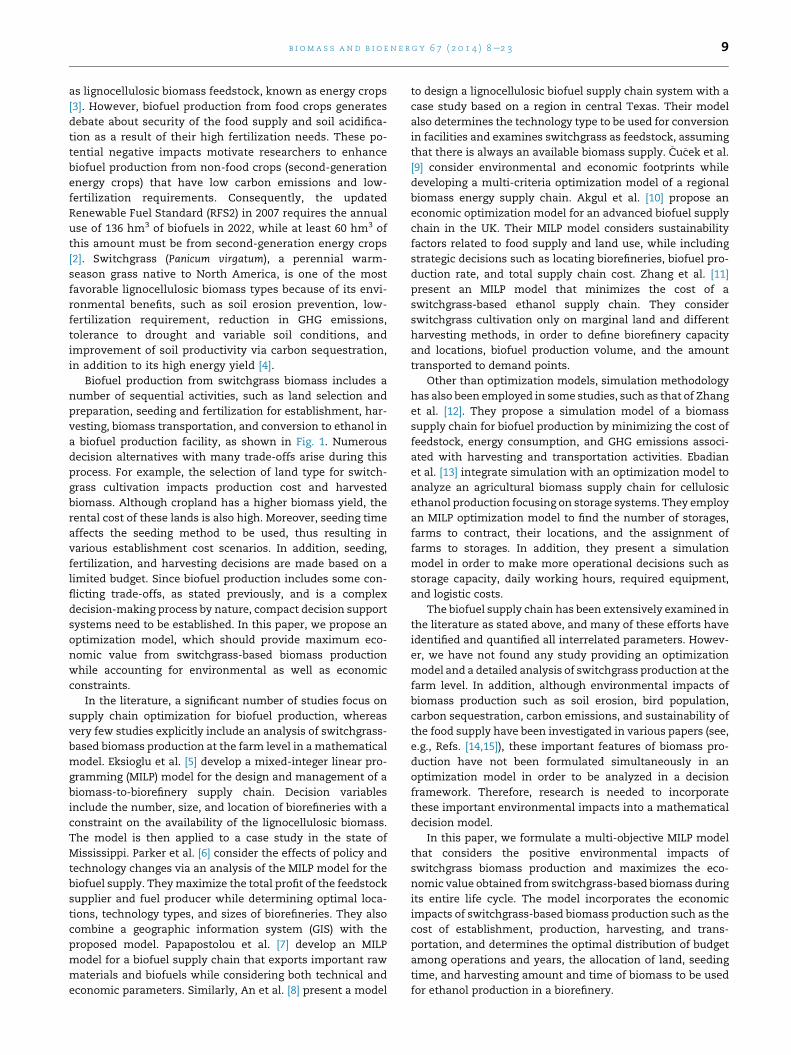
Fig. 1 e Operation types included in biofuel production from switchgrass.

b i om a s s a n d b i o e n e r g y 6 7 ( 2 0 1 4 ) 8e2 310

In addition, the proposed mathematical model contributes

to the state of the art by considering the following aspects:

� To our knowledge, none of the reviewed literature con-

siders the seeding scenario, including seeding season and

seeding method. Each seeding scenario has a different cost

and leads to various yield amounts. The proposed model

determines the best seeding scenario including seeding

season and seeding method in order to produce the

maximum amount of yield given a limited budget.

� Again, to the best of our knowledge, none of the previous

work considers the environmental contributions of

switchgrass in a biomass production optimization model.

As stated by Hartman et al. [16], switchgrass cultivation

can be considered on degraded and marginal land that are

in a conservation reserve program (CRP) since switchgrass

can restore the soil quality through increasing its organic

carbon content. In addition, having a very strong root

system, switchgrass prevents soil erosion significantly,

which in turn provides savings from reduced loss of fertile

soil. The proposed model incorporates switchgrass pro-

duction in productive as well as degraded land and ana-

lyzes its positive impacts on soil erosion prevention.

� This study also fills the gap of investigating and controlling

the effect of harvesting patterns on grassland bird pop-

ulations. It has been shown that rotational harvesting is

required in order to provide a nesting area to birds during

winter [16,17]. Ourmodel handles sustainability of bird and

wildlife populations by providing them available habitats

through limiting the number of harvested regions.

� In the literature, land allocation is defined with respect to

the amount of area needed for cultivation, and in most

cases, cropland is used for the cultivation of biomass crops.

The model proposed by An et al. [8] determines the

biomass amount required, where biomass is assumed to be

provided from cropland and lands in a CRP. On the other

hand, Zhang et al. [11] limit the cultivation of switchgrass

production to only marginal land. Our model is differenti-

ated from others by leaving the choice of land type to

decision-makers (landowners), since they can control

cropland, grassland (pastureland), and marginal land in

coordination. The model also enables decision-makers to

quantify the availability of cropland to be used for

switchgrass cultivation by incorporating a sustainability

factor in the land-usage constraints.

� In this model, we have calculated the establishment cost

for various seeding scenarios and production cost, which

depend on the rental cost and the amount of fertilizers

used. Furthermore, the savings from soil erosion preven-

tion and CO2 retained via soil carbon storage, which are not

directly available in the literature, are calculated by

incorporating a couple of sources. Therefore, this paper

also provides compact data for researchers looking for

various aspects of environmental and economic input and

output of switchgrass biomass production.

� In the literature, many constraints are not directly avail-

able: growth function of the switchgrass population; cost of

production including fertilizers; harvesting cost including

cost ofmowing, raking, baling, staging, and loading; as well

as the limitation of harvested areas to ensure sustainability

of bird populations. In order to incorporate these con-

straints into our optimization model, we have generated

formulations by evaluating the research-based in-

structions and data available in the literature. Althoughwe

have established the model particularly for switchgrass, it

can also be used as a basis for and applied to biomass

production from any other types of energy crops.

The remainder of this paper is organized as follows. The

problem is defined in section 2, while themathematicalmodel

is described in detail in section 3. The calculation of input

parameters and the application of the model to a real case

study in Kansas are presented in section 4. All computational

results for the base-case scenario and sensitivity analyses are

given in section 5. Finally, some concluding remarks with

future directions are provided in section 6.

2. Problem statement

We focus on the following echelons for the switchgrass-

based biofuel production shown in Fig. 1: land allocation,

establishment, biomass production, biomass harvesting,

and its transportation to a biorefinery. The land types to be

allocated for switchgrass cultivation include cropland,

grassland, and marginal land. Cropland defines the pro-

ductive land where food crops are cultivated. Grassland is

considered to have semi-productive soil covered by grasses.

Marginal land refers to arid, degraded soil and lands that are

in a CRP. After land type is determined, a seeding season

(frost and spring) and a suitable seeding method (airflow,

drill, and no-till drill) are decided. Harvesting, which in-

cludes mowing, raking, baling, staging, and loading, is per-

formed by late September. Finally, the harvested

switchgrass biomass is transported to the biorefinery to be

converted into bioethanol.

The objective of the mathematical model is to maximize

the total economic value obtained from switchgrass biomass

production while determining the optimal decision strategies

for the following:

b i om a s s a n d b i o e n e r g y 6 7 ( 2 0 1 4 ) 8e2 3 11

� Land allocation (seeding zones) for switchgrass cultivation.

� Seeding time along with seeding scenario to be

implemented.

� Biomass cultivated zones to be harvested and time for

harvesting.

� Amount of harvested switchgrass in a related zone at the

time of harvesting.

� Allocation of budget to various farm operations (seeding,

production, harvesting, and transportation).

2.1. Notation and assumptions

Depending on the equipment used, the estimation of har-

vesting cost can vary considerably. The type of bale (large

round or large square) also affects the cost. For the budget

Nomenclature

Indices

i row of cultivation zone

j column of cultivation zone

(i, j) switchgrass cultivation zone

k switchgrass seeding scenario

t time period

l transportation mode

Sets

I set of rows of cultivation area

J set of columns of cultivation area

K set of seeding scenarios

T set of time periods in planning horizon

L set of transportation modes

Mt set of time periods from the first period to period t

(Mt ¼ {1, ., t})

CR set of cultivation zones on croplands in cultivation

area

Binary decision variables

Stijk 1 if zone (i, j) is seeded at time period t with

seeding scenario k, and 0 otherwise

Xtij 1 if zone (i, j) is harvested at time period t, and

0 otherwise

Continuous decision variables

Ntij switchgrass yield in zone (i, j) at time period t (t)

Ntij harvested switchgrass biomass in zone (i, j) at

time period t (t)

Eb establishment budget ($)

Pb production budget ($)

Hb harvesting budget ($)

Tb transportation budget ($)

Parameters

Pt sale price of switchgrass at time period t ($ t�1)

SEij soil erosion prevention economic value of

switchgrass in zone (i, j) in each period ($)

CSij carbon sequestration economic value of

switchgrass in zone (i, j) in each period ($)

estimations in this paper, we consider harvesting in large

square bales weighing 397 kg each, which are easy to trans-

port and store [18,19].

Studies show that multiple harvesting in the same year

decreases the total amount of biomass since the root system is

weakened [19,20]. Therefore, single harvesting, which is sug-

gested immediately after the first killing frost, is used in this

model because it is stated to be the most economical and

environmentally friendly harvesting method [11].

It has been shown that bioethanol producers prefer to

obtain their biomass supply from within an 80-km radius of

the biorefinery, due to the high cost of transporting bulky

biomass [5]. Therefore, this study aims to maximize the

economic value of switchgrass production, given that a

predetermined facility is located in close proximity to the

cultivation area.

sk carbon emissions penalty for seeding

scenario k ($)

r fixed carbon emissions penalty for production and

harvesting ($)

u variable carbon emissions penalty specific for

production and harvesting ($ t�1)

s carbon emissions penalty for biomass

transportation ($ t�1 km�1)

a weight of switchgrass sales

b weight of soil erosion prevention value

m weight of savings from the reduction of GHG

emissions via carbon sequestration

Aij potential switchgrass yield from zone (i, j) (t)

pt growth factor of switchgrass after t years of

establishment

D fraction of facility capacity assigned to biomass

from switchgrass

Capt biomass capacity of facility at time period t (t)

TECk total expected establishment cost for seeding

scenario k ($)

MCk machinery cost for seeding scenario k ($)

SCk seeding cost for seeding scenario k ($)

FCk fertilization cost for seeding scenario k ($)

PCk pesticide cost for seeding scenario k ($)

RECk re-establishment cost of seeding scenario k ($)

Rk re-establishment probability of seeding scenario k

j fixed cost of switchgrass production per

cultivation zone ($)

g variable cost of switchgrass production ($ t�1)

RCij rental cost of cultivation zone (i, j) ($)

d fixed cost of harvesting per zone ($)

q variable cost of harvesting ($ t�1)

Dij distance of zone (i, j) to facility (km)

Fl fixed cost of transportation mode l ($)

Vl variable cost of transportation mode l ($ t�1 km�1)

Ab total available budget in the planning horizon ($)

l sustainability factor defining the percentage of

cropland, which is not allowed for biomass

production

b i om a s s a n d b i o e n e r g y 6 7 ( 2 0 1 4 ) 8e2 312

3. Mathematical modeling

AnMILPmodel is formulatedwith the objective ofmaximizing

economic values obtained from switchgrass-based biomass

production as well as its beneficial environmental impacts.

The optimal levels for various decisions regarding seeding and

harvesting time periods and cultivation areas are determined

by solving the MILP model. A detailed explanation of the

objective function and the constraints of the proposed model

are given in the following sections.

3.1. Objective function

The objective of the proposed model is the maximization of

the weighted sum of the total economic value obtained from

switchgrass production. The total economic value (TEV) in-

cludes revenue to be obtained from the sales of switchgrass

biomass (TB), economic value of soil erosion prevention (TS),

and savings from the reduction of GHG emissions via carbon

sequestration (TC), as indicated below:

TEV ¼ aTBþ bTSþ mTC (1)

All terms aremultiplied by a, b, and m, respectively, in order

to assign the priorities of the decision-maker where the sum

of a, b, and m equals 1. The first term, direct revenue of the

farmer from the sales of biomass production, is calculated as

TB ¼Xi˛I

Xj˛J

Xt˛T

Nt

ijPt (2)

where Nt

ij is the amount of harvested switchgrass biomass in

zone (i, j) at time t, and Pt is the sale price of switchgrass

biomass at time t.

We also need to consider the cost of soil erosion to land-

owners and farmers. In most cases, farmers rent land from

owners. Independent of whether the farmer is the owner or not,

more fertilizer is needed to compensate for the impact of soil

erosion, and eventually land value decreases due to loss of pro-

ductivity. Studies show that growing switchgrass reduces soil

erosion significantly [21,22]. Therefore, the second term repre-

sents savings from soil erosion via switchgrass cultivation as

TS ¼Xi˛I

Xj˛J

Xt˛T

Ntij

AijSEij (3)

where the ratio of Ntij to Aij is the percentage of switchgrass

yield grown at time twith respect to the potential yield in zone

(i, j), and SEij is the economic value of the soil erosion pre-

vention in zone (i, j) in each period.

Finally, since the storage of atmospheric CO2 as soil organic

carbon (SOC) increases the soil quality and since carbon

sequestration can be potentially used as savings in carbon

emission trading systems, the net CO2 sequestration is also

evaluated as a benefit of switchgrass cultivation [23,24]. The last

term, TC, savings from net carbon emission reduction, is

calculated by

TC ¼Xi˛I

Xj˛J

Xt˛T

Nt

ij

AijCSij �

Xk˛K

Stijksk � Xt

ijr�Nt

ij

�uþ Dijs

�!(4)

where CSij is the economic value of carbon sequestered in

zone (i, j) in each period, sk is the carbon emissions penalty for

seeding scenario k, r is the carbon emissions penalty for

production operations depending on harvesting, while u is the

carbon emissions penalty for production operations depend-

ing on yield. Finally, s is the carbon emissions penalty for

transporting harvested biomass.

3.2. Production constraints

Total switchgrass amount grown in zone (i, j) in year t, Ntij, is

defined as

Ntij ¼

Xk˛K

Xz˛Mt

Aijpt�zþ1Sz

ijk c i; j; t (5)

where Aij is the potential switchgrass yield in zone (i, j), Stijk is

the binary variable defining seeding scenario k in zone (i, j) at

time t, and pt�zþ1 is the switchgrass growth factor. It takes

three years for switchgrass to reach its potential yield [19].

Therefore, pt�zþ1 shows the portion of potential switchgrass

yield reached by time period t, where z represents the time

period of seeding.

The total number of seedings at each zone (i, j) is limited to

one, and only one seeding scenario k can be used through

period t:

Xk˛K

Xt˛T

Stijk � 1 c i; j (6)

Harvesting at each zone (i, j) at time t can only be made if

that zone is already seeded through time period t by any

seeding scenario k as

Xtij �

Xk˛K

Xz˛Mt

Szijk c i; j; t (7)

Harvested switchgrass biomass in zone (i, j) at time period

t, Nt

ij, cannot exceed the amount of switchgrass grown, Ntij, in

that zone:

Nt

ij � Ntij c i; j; t (8)

On the other hand, the harvested switchgrass biomass

in zone (i, j) at time period t can be, at most, equal to the

potential switchgrass yield of zone (i, j), if Xtij is set to 1. If

there is no harvest at time t, i.e., if Xtij is set to zero, then N

t

ij

is zero:

Nt

ij � AijXtij c i; j; t (9)

The total amount of the harvested biomass in each period

is limited by the capacity of the facility:

Xi˛I

Xj˛J

Nt

ij � DCapt c t (10)

where D is the fraction of facility capacity assigned to biomass

from switchgrass, and Capt is the biomass capacity of the fa-

cility at time period t.

3.3. Budget constraints

The budget assigned for establishment, Eb, is defined by the

total establishment cost of seeding in all zones (i, j) for all

seeding scenarios k in the planning horizon as

b i om a s s a n d b i o e n e r g y 6 7 ( 2 0 1 4 ) 8e2 3 13

Eb ¼Xi˛I

Xj˛J

Xk˛K

Xt˛T

TECkStijk (11)

where switchgrass establishment cost, TECk, is the sum of

machinery, seeding, fertilization, and pesticide costs for

seeding scenario k, as well as the expected re-establishment

cost, RECk, of a failed establishment trial. In order to find the

expected establishment cost, RECk is multiplied by Rk, the

probability of establishment failure for seeding scenario k.

TECk is used as an input and computed as

TECk ¼ MCk þ SCk þ FCk þ PCk þ RECkRk c k (12)

The budget assigned for production, Pb, is defined by the

total production cost of switchgrass cultivation as

Pb ¼Xi˛I

Xj˛J

Xt˛T

jXt

ij þ gNt

ij þXk˛K

Xz˛Mt

SzijkRCij

!(13)

where j is the fixed cost of nitrogen (N) application, and g is

the variable cost for phosphorus (P) and potassium (K) appli-

cations, since a fixed amount of N after harvesting and vari-

able amounts of P and K for each tonne of harvested biomass

are suggested for the best production practices of switch-

grass [18,19]. The term RCij, the rental cost of zone (i, j), is

multiplied by the seeding decision variable, which becomes 1

if switchgrass is seeded in that zone, and 0 otherwise.

Similarly, the budget assigned for harvesting, Hb, is defined

by the overall cost of harvesting as

Hb ¼Xi˛I

Xj˛J

Xt˛T

�dXt

ij þ qNt

ij

�(14)

where the total harvesting cost consists of the fixed cost, d, of

harvesting, and variable cost, q, which depends on the amount

of harvested switchgrass biomass. Mowing and raking have a

fixed cost per harvested zone, while the cost of baling, staging,

and loadingdependson theharvestedswitchgrassbiomass [19].

Various available transportation modes can be used to

transport biomass to the biorefinery facility. The budget

assigned for transportation, Tb, is defined as the total ex-

penses related to transportation as

Tb ¼Xi˛I

Xj˛J

Xt˛T

Xl˛L

�FlX

tij þ VlDijN

t

ij

�(15)

where Fl is the fixed cost incurred for the chosen trans-

portation mode l, if zone (i, j) is harvested, and Vl represents

the variable cost of mode l, which depends on the distance to

the biorefinery and the harvested biomass amount [19].

The total cost of farm operationsdestablishment, pro-

duction, harvesting, and transportationdwhich are given in

detail in equations (11)e(15), cannot exceed the total available

budget, Ab, in the planning horizon, as given below:

Eb þ Pb þ Hb þ Tb � Ab (16)

Equation (16) is formulized in the model in order to deter-

mine the value of optimal budget allocation to establishment,

production, harvesting, and transportation operations.

3.4. Environmental constraints

We formulate environmental constraints, considering the

ecological consequences of switchgrass production, with the

purpose of maintaining biodiversity and providing food sup-

ply safety.

The following constraint is introduced to the model to

sustain continuity and diversity of bird populations:

Xiþ1

m¼i�1

Xjþ1

n¼j�1

�1� Xt

mn

� � Xtij c i; j; t (17)

Constraint (17) ensures that if zone (i, j) is harvested, then

one of its neighbor zones should remain unharvested in each

time period t to ensure a nesting area for birds during winter.

It has been also stated that diversity of bird species increases

only when there is a mixture of harvested and unharvested

fields in a region, since shortgrass bird populations grow on

harvested fields, while tallgrass bird populations can survive

better on unharvested fields [16,17].

For sustainability of the food supply, a particular percent-

age of cropland should be kept for food crop production. Zones

to be converted to energy crop production cannot exceed the

allowable share, 1�l, of cropland:

Xði;jÞ˛CR

Xk˛K

Xt˛T

Stijk � ð1� lÞ jCR j (18)

where jCRj refers to the cardinality of the set of croplands.

4. Case study

TheMILPmodel explained in section 3 has been applied to the

case of a biofuel production project in Hugoton, Kansas. The

project was announced by the United States Department of

Agriculture as one of the Biomass Crop Assistance Program

projects in 2011. The proposed area to be used for biomass

production from switchgrass is up to 8094 ha and is sponsored

by Abengoa Bioenergy LLC. This planned biorefinery has

95 hm3 of cellulosic ethanol capacity through the conversion

of 330,000 t of crops [25,26].We assumed an ample capacity for

the biorefinery, which does not limit the biomass production,

where full capacity is assigned to biomass obtained from

switchgrass. The cultivation area surrounding the biorefinery

in the center of Hugoton has three different soil types: crop-

land, grassland, and CRP land, which we consider as marginal

land in this study. The total area is divided into 21 by 21

rectangular arrays, leading to 441 zones, each 2.59 km2 (1

square mile) in size. A total of 11 seeding scenarios have been

evaluated in this case study. Since the expected life of

switchgrass is at least ten years, in order to obtain the

maximum utilization of the investment on switchgrass pro-

duction, the planning horizon is considered as ten years in

this case study [29]. The other necessary input parameters

used in the model are provided with detailed explanations in

the next section.

4.1. Input parameters

In this section, we present the data collected from various

resources in order to formulate our case study. Since we have

different land types and seeding scenarios, for some param-

eters, we have consulted a combination of various publicly

Table 1 e Seeding scenarios and corresponding yield amounts.

Seeding scenario Seeding scenario characteristics Yield (t ha�1)

Land type Seeding season Method t ¼ 1 t ¼ 2 t ¼ 3e10

1 Cropland Frost Airflow 3.75 10 15

2 Grassland Frost Airflow 2.63 7 10.5

3 Cropland Spring Airflow 3.75 10 15

4 Cropland Spring Drill 3.75 10 15

5 Cropland Spring No-till drill 3.75 10 15

6 Grassland Spring Drill 2.63 7 10.5

7 Grassland Spring No-till drill 2.63 7 10.5

8 Marginal land Frost Airflow 1.87 5 7.5

9 Marginal land Spring Airflow 1.87 5 7.5

10 Marginal land Spring Drill 1.87 5 7.5

11 Marginal land Spring No-till drill 1.87 5 7.5

b i om a s s a n d b i o e n e r g y 6 7 ( 2 0 1 4 ) 8e2 314

available sources in order to gather and calculate the data. The

next subsections include those references that we have used

for the purpose of data collection. This section also provides a

valuable asset to researchers looking for compact data in this

field.

4.1.1. Seeding scenarios and yieldsSeeding scenarios and corresponding yield amounts for each

scenario in different years are given in Table 1. Seeding sce-

narios are defined by three characteristics: land type, seeding

season, and seeding method. Land type includes cropland,

grassland, andmarginal land. There are two available seeding

seasons: frost seeding and spring seeding. For seeding

method, airflow and no-till drill are used as modern seeding

methods because they lead to low soil erosion and less carbon

emissions, in contrast to drill seeding, which is used as the

conventional (traditional) seeding method. In this study, we

add four seeding scenarios of marginal land to those seven

scenarios provided for cropland and grassland by Duffy and

Nanhou [18].

The amount of switchgrass yield is mostly affected by land

type and time passed since the establishment. Various yield

amounts, ranging from 10 to 20 t ha�1 y�1, are estimated for

cropland. In this case study, for cropland, we use an average

value, 15 t ha�1 y�1 as the potential yield, which is a practical

amount in Kansas [27,28]. We also consider lower and upper

bound values on the yield level in the computational experi-

ments in order to investigate the impact of possible changes in

Table 2 e Switchgrass establishment, re-establishment, and to

Seedingscenario

Establishment cost($ ha�1)

Re-establishment($ ha�1)

1 407.15 112

2 417.77 112

3 416.84 112

4 589.35 121.4

5 505.60 116

6 599.97 121.4

7 516.62 116

8 446.80 112

9 426.53 112

10 599.97 121.4

11 516.62 116

yield level. The potential switchgrass yield is reached at the

third year after establishment [19]. The first-year switchgrass

yields may only be 25% of the potential yield. In the second

year of establishment, biomass yields can reach 66% of the

potential yield, based on the discussion by Garland et al. [29]

and West and Kincer [30]. For instance, in order to obtain

the yield amount in cropland in the first year, the potential

yield (15 t) is multiplied by 25%, thus leading to 3.75 t, while it

is multiplied by 66% to calculate the yield amount in the

second year. On the other hand, the yield of grassland and

marginal land drops to 70% and 50%, respectively, of that in

cropland [31]. For instance, to compute the amount of

switchgrass yield in marginal land in the first year, 3.75 t is

multiplied by 50%.

4.1.2. Establishment cost and selling priceData regarding the establishment and re-establishment costs

for various scenarios are provided in Table 2 [18,19]. The

selling price of switchgrass is taken as $120 t�1 [32], while

establishment cost depends on many variables such as ma-

chinery, seed, fertilizer, and pesticide costs. In machinery

cost, grassland seeding scenarios (2, 6, and 7) include the cost

of additional Roundup spraying to prepare the land for culti-

vation. Pure live seed (PLS) in the amounts of 6.7 kg ha�1 and

5.6 kg ha�1 is used for frost seeding and spring seeding,

respectively, in both cropland and grassland. PLS in the

amount of 11.2 kg ha�1 and 8.9 kg ha�1 are used for frost and

spring seeding, respectively, in marginal land. Phosphorus (P)

tal expected establishment costs.

cost, RECk Total expected establishment cost, TECk

($ ha�1)

435.15

445.77

472.84

650.05

563.60

660.67

574.62

474.80

482.53

660.67

574.62

Table 3 e Soil organic carbon (SOC), CO2 equivalence, andsavings.

Seedingscenario

SOC(t ha�1 y�1)

CO2 equivalence(t ha�1 y�1)

Savings($ ha�1 y�1)

1, 3, 4, 5 4.42 16.22 324.4

2, 6, 7 0.32 1.17 23.5

8, 9, 10, 11 3.2 11.74 234.8

b i om a s s a n d b i o e n e r g y 6 7 ( 2 0 1 4 ) 8e2 3 15

in the amount of 33.6 kg ha�1 and potassium (K) in the amount

of 44.8 kg ha�1 are applied for establishment. Nitrogen (N)

fertilizer is usually not applied during the seeding year

because this tends to stimulate weed growth more than

switchgrass growth. Atrazine and 2,4 D pesticides are used on

all types of lands.

Re-establishment is required if there are not enough

switchgrass stands a year later than seeding. Re-

establishment cost consists of seeding, fertilizer, pesticide,

and machinery costs. Since Roundup is already used for land

preparation in establishment, it is not included in re-

establishment cost. The probability of re-establishment is

taken as 25% for frost seeding and 50% for spring seeding

scenarios, as suggested in the literature [18]. Re-establishment

cost is multiplied by the corresponding probability values and

added to the establishment cost in order to compute the ex-

pected cost of establishment.

4.1.3. Production costAnnual production cost includes rental, fertilizer, and pesti-

cide costs. Average land rental costs for 1 ha of cropland,

grassland, and marginal land in southwest of Kansas are

$234.6, $23.7, and $75.3 [33], respectively. Fertilizers P and K

are applied in the amounts of 0.42 kg and 9.47 kg, respectively,

for each tonne of switchgrass harvested. A moderate amount

of N (112 kg ha�1) is used in this case study. Nitrogen appli-

cation costs $137 ha�1, while each kg of K and P costs $12. The

cost of pesticide is $16.89 ha�1 [18].

4.1.4. Harvesting costThe harvesting operation includes mowing, raking, baling,

staging, and loading. For the budget estimations in this paper,

it is assumed that harvesting is done in large square bales

weighing 397 kg each. Mowing and raking has a fixed cost of

$31.61 ha�1. The cost of baling is $7, while the cost of staging

and loading is $2.8, leading to a total of $9.8 for each bale [18].

Since 2.5 bales are obtained for each tonne, the variable cost of

harvesting is taken as $24.5 t�1 of switchgrass harvested.

4.1.5. Transportation costThe cost of transporting the biomass by truck is calculated

based on the following formula: $5.70 þ 0.1367X, where X is

the distance of the cultivation zone to the facility in km, while

0.1367 is the variable cost in $ km�1 t�1. On the other hand,

transporting the biomass by rail costs $17.10 þ 0.0277X [19]. In

this study, distance to the facility is calculated based on a city-

block distance, also known as theManhattan distance. Among

the transportation modes, only one mode of transportation,

transportation by truck is considered for this specific case

because of its availability in Kansas.

4.1.6. Soil erosionParameter values regarding the environmental benefits of

switchgrass cultivation have also been computed. A recent

study of the U.S. Department of Agriculture (USDA) considers

farmer and societal costs of soil erosion by providing scien-

tifically derived estimates. Summing the values of fertilizer

saved ($1.95) and water quality benefits ($5.43), the USDA es-

timates that the yearly savings of the farmers and society

from erosion is equal to $7.38 for each tonne of soil [21]. The

USDA estimates soil erosion in Kansas to be 8.29, 1.34, and

2.69 t ha�1 for cropland, grassland, and marginal land,

respectively. Multiplying these amounts by $7.38, value of one

tonne of soil per year, we estimate soil-erosion savings via

switchgrass cultivation to be $61.18, $9.89, and $19.85 ha�1 y�1

for cropland, grassland, and marginal land, respectively.

4.1.7. Carbon sequestration and CO2 emissionsThe amount of soil organic carbon (SOC) sequestered, its CO2

equivalence, and saving values due to carbon sequestration for

each seeding scenario are given in Table 3. SOC sequestration

depends on soil type. The value of SOC sequestration in crop-

land is taken as 4.42 t ha�1 y�1 [34]. On the other hand, seques-

tration rates of up to 2.4e4.0 t ha�1 y�1 are reported for

switchgrass crop grown in the CRP in South Dakota [35].

Therefore, an average value of 3.2 t ha�1 y�1 is used for carbon

sequestration on marginal land. Since grassland is expected to

be already saturated with high concentration of SOC, carbon

sequestrationvia switchgrasscultivation is less than1 tha�1 y�1

[36]. In this study, it is assumed to be 10% of that is onmarginal

land. To compute the equivalent CO2 sequestered from the at-

mosphere, the SOC values in Table 3 are multiplied by 3.67 [37].

The average cost of CO2 emissions is $20 t�1, according to the

emissions trading system in the EU [38]. The savings column is

computed bymultiplying CO2 equivalence with $20 t�1.

Carbon emissions that occur during seeding, production,

harvesting, and transportation operations are given in Table

4 [39,40]. CO2 emitted during in each sub-operation including

pesticide or fertilizer application is given under the CO2

emissions column. The number (amount) of these sub-

operations (pesticides or fertilizers) in each operation is indi-

cated in the usage column. Finally, the cost of CO2 emissions is

presented in the cost column and is equal to the multiplica-

tion of CO2 emissions, usage, and $20 t�1. For instance, the

cost of pesticide application in the seeding operation is ob-

tained by 6.3(kg kg�1) * 5.25(kg ha�1) * $20 t�1, which equals

$0.66 ha�1.

As given in equation (4), the net savings from CO2

sequestration are obtained by subtracting the cost of carbon

emissions in Table 4 from the savings via CO2 sequestration in

Table 3.

4.2. Experimental design

In this section, we evaluate the impact of key parameters on

results. These parameters include the objective function

weights, yield levels, sustainability factor, and the available

budget amount for biomass production.

We investigate three different cases of weight selection for

(a, b, and m) in the objective function given in equation (1) in

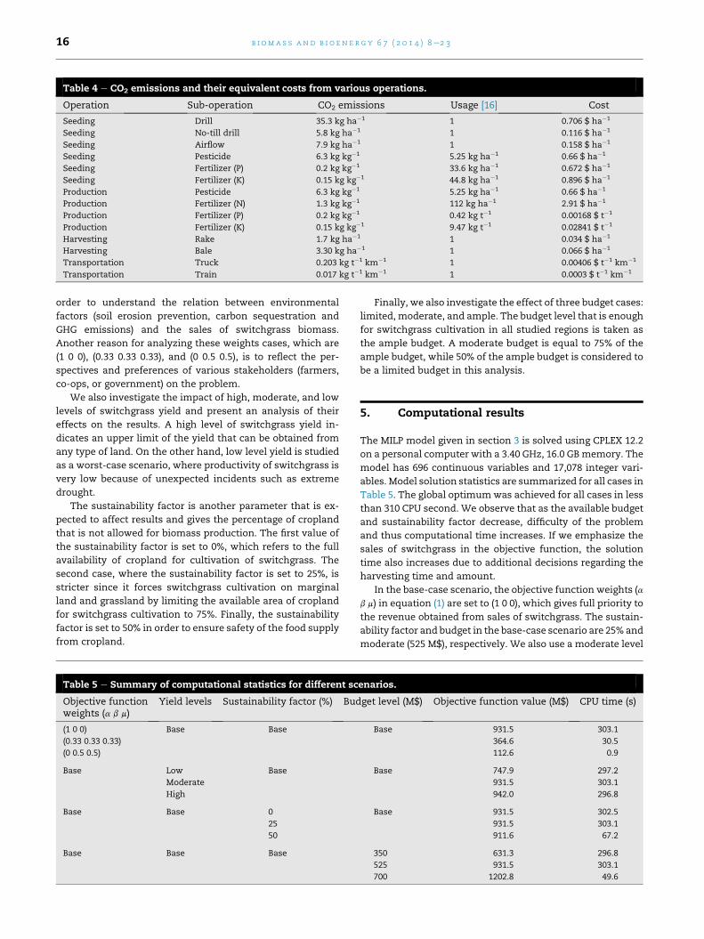
Table 4 e CO2 emissions and their equivalent costs from various operations.

Operation Sub-operation CO2 emissions Usage [16] Cost

Seeding Drill 35.3 kg ha�1 1 0.706 $ ha�1

Seeding No-till drill 5.8 kg ha�1 1 0.116 $ ha�1

Seeding Airflow 7.9 kg ha�1 1 0.158 $ ha�1

Seeding Pesticide 6.3 kg kg�1 5.25 kg ha�1 0.66 $ ha�1

Seeding Fertilizer (P) 0.2 kg kg�1 33.6 kg ha�1 0.672 $ ha�1

Seeding Fertilizer (K) 0.15 kg kg�1 44.8 kg ha�1 0.896 $ ha�1

Production Pesticide 6.3 kg kg�1 5.25 kg ha�1 0.66 $ ha�1

Production Fertilizer (N) 1.3 kg kg�1 112 kg ha�1 2.91 $ ha�1

Production Fertilizer (P) 0.2 kg kg�1 0.42 kg t�1 0.00168 $ t�1

Production Fertilizer (K) 0.15 kg kg�1 9.47 kg t�1 0.02841 $ t�1

Harvesting Rake 1.7 kg ha�1 1 0.034 $ ha�1

Harvesting Bale 3.30 kg ha�1 1 0.066 $ ha�1

Transportation Truck 0.203 kg t�1 km�1 1 0.00406 $ t�1 km�1

Transportation Train 0.017 kg t�1 km�1 1 0.0003 $ t�1 km�1

b i om a s s a n d b i o e n e r g y 6 7 ( 2 0 1 4 ) 8e2 316

order to understand the relation between environmental

factors (soil erosion prevention, carbon sequestration and

GHG emissions) and the sales of switchgrass biomass.

Another reason for analyzing these weights cases, which are

(1 0 0), (0.33 0.33 0.33), and (0 0.5 0.5), is to reflect the per-

spectives and preferences of various stakeholders (farmers,

co-ops, or government) on the problem.

We also investigate the impact of high, moderate, and low

levels of switchgrass yield and present an analysis of their

effects on the results. A high level of switchgrass yield in-

dicates an upper limit of the yield that can be obtained from

any type of land. On the other hand, low level yield is studied

as a worst-case scenario, where productivity of switchgrass is

very low because of unexpected incidents such as extreme

drought.

The sustainability factor is another parameter that is ex-

pected to affect results and gives the percentage of cropland

that is not allowed for biomass production. The first value of

the sustainability factor is set to 0%, which refers to the full

availability of cropland for cultivation of switchgrass. The

second case, where the sustainability factor is set to 25%, is

stricter since it forces switchgrass cultivation on marginal

land and grassland by limiting the available area of cropland

for switchgrass cultivation to 75%. Finally, the sustainability

factor is set to 50% in order to ensure safety of the food supply

from cropland.

Table 5 e Summary of computational statistics for different sc

Objective functionweights (a b m)

Yield levels Sustainability factor (%) Bud

(1 0 0) Base Base

(0.33 0.33 0.33)

(0 0.5 0.5)

Base Low Base

Moderate

High

Base Base 0

25

50

Base Base Base

Finally, we also investigate the effect of three budget cases:

limited, moderate, and ample. The budget level that is enough

for switchgrass cultivation in all studied regions is taken as

the ample budget. A moderate budget is equal to 75% of the

ample budget, while 50% of the ample budget is considered to

be a limited budget in this analysis.

5. Computational results

The MILP model given in section 3 is solved using CPLEX 12.2

on a personal computer with a 3.40 GHz, 16.0 GBmemory. The

model has 696 continuous variables and 17,078 integer vari-

ables. Model solution statistics are summarized for all cases in

Table 5. The global optimumwas achieved for all cases in less

than 310 CPU second. We observe that as the available budget

and sustainability factor decrease, difficulty of the problem

and thus computational time increases. If we emphasize the

sales of switchgrass in the objective function, the solution

time also increases due to additional decisions regarding the

harvesting time and amount.

In the base-case scenario, the objective function weights (a

b m) in equation (1) are set to (1 0 0), which gives full priority to

the revenue obtained from sales of switchgrass. The sustain-

ability factor and budget in the base-case scenario are 25% and

moderate (525 M$), respectively. We also use a moderate level

enarios.

get level (M$) Objective function value (M$) CPU time (s)

Base 931.5 303.1

364.6 30.5

112.6 0.9

Base 747.9 297.2

931.5 303.1

942.0 296.8

Base 931.5 302.5

931.5 303.1

911.6 67.2

350 631.3 296.8

525 931.5 303.1

700 1202.8 49.6

Fig. 2 e Hugoton area divided into 21 by 21 zones including land types, facility, residential areas, and optimal switchgrass

seeding locations.

Fig. 3 e Biomass yield and harvested amount in the

planning horizon.

b i om a s s a n d b i o e n e r g y 6 7 ( 2 0 1 4 ) 8e2 3 17

of switchgrass yield, which is given in Table 1, in the base-case

scenario. The first four columns of Table 5 correspond to four

different parameters that are investigated. In Table 5, four

different sets of experiments are presented in each row-block

of the table. In each set of experiments, each parameter is set

to three different values, as explained in section 4.2, in order

to analyze its impact on the results, while the remaining pa-

rameters are fixed to the base case values.

Whenwe analyze the tightness of the constraints given the

optimal solution in the base case, we observe that total

switchgrass yield is equal to the potential switchgrass yield

(constraint (5)), while harvested switchgrass biomass is equal

to switchgrass yield (constraint (8)). Constraints (6), (7) and (9)

are also binding. Inequality (10) is not a limiting constraint

since we have considered an ample capacity in this case

study. All constraints (11)e(16) regarding the budget allocation

are binding. Inequality (17) limits harvested zones to ensure

sustainability of bird populations, while constraint (18) is not

binding in the base case since cropland utilization is already

less than 75%.

As mentioned in section 4, the model is applied to a case

study in Hugoton. Fig. 2 displays amap of the studied region in

Hugoton, which is divided into 21 by 21 rectangular arrays of

cultivation zones with the row and column numbers referring

to zone (i, j) in themodel. For example, zone (11, 11) shows the

location of the facility, which is in the center of the Hugoton

map, while cultivation zone (6, 9) shows one section of

grassland in the considered region. This map displays the

considered area with the distribution of land types, the loca-

tion of the facility, and residential areas while indicating

optimal seeding zones in the first year of the planning horizon

when the MILP model is solved for the base-case scenario. It

can be seen that the closest zones to the facility are selected

for switchgrass cultivation. In addition, grassland is selected

for cultivation since it has a lower rental cost while cropland

becomes favorable due to its higher switchgrass yield. As the

best seeding scenario, scenario 1 is selected for cropland,

while scenario 2 is chosen for grassland. Both of these sce-

narios involve airflow planting in frost seeding. Seeding time

is always chosen as the first year of the planning horizon in

order to increase the overall production amount. Out of 248

zones of cropland, 163 are utilized for switchgrass production,

while 93 out of 94 zones of grassland are converted into

switchgrass cultivation. In other words, 87.6% of available

cropland is used, while this value increases to 99% for grass-

land. For this case, none of the 88 zones of marginal land is

chosen for switchgrass cultivation. The total area converted to

switchgrass cultivation is as follows: 42,380 ha for cropland

and 24,180 ha for grassland. The overall amount of biomass

yield reaches 7.99 Mt, while 7.76 Mt of that amount is har-

vested in the ten-year planning horizon. The cost of switch-

grass biomass harvested is calculated as $67.63 t�1 for the

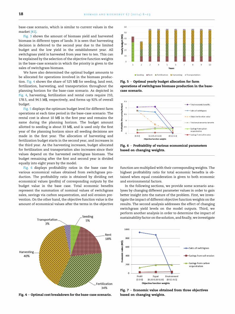
Fig. 5 e Optimal yearly budget allocation for farm

operations of switchgrass biomass production in the base-

case scenario.

Fig. 6 e Profitability of various economical parameters

based on changing weights.

b i om a s s a n d b i o e n e r g y 6 7 ( 2 0 1 4 ) 8e2 318

base-case scenario, which is similar to current values in the

market [41].

Fig. 3 shows the amount of biomass yield and harvested

biomass in different types of lands. It is seen that harvesting

decision is deferred to the second year due to the limited

budget and the low yield in the establishment year. All

switchgrass yield is harvested from year two to ten. This can

be explained by the selection of the objective functionweights

in the base-case scenario in which the priority is given to the

sales of switchgrass biomass.

We have also determined the optimal budget amounts to

be allocated for operations involved in the biomass produc-

tion. Fig. 4 shows the share of 525 M$ for seeding, land rent,

fertilization, harvesting, and transportation throughout the

planning horizon for the base-case scenario. As depicted in

Fig. 4, harvesting, fertilization and rental costs require 210,

178.5, and 94.5 M$, respectively, and forms up 92% of overall

budget.

Fig. 5 displays the optimum budget level for different farm

operations at each time period in the base-case scenario. The

rental cost is about 10 M$ in the first year and remains the

same during the planning horizon. The budget amount

allotted to seeding is about 33 M$, and is used only the first

year of the planning horizon since all seeding decisions are

made in the first year. The allocation of harvesting and

fertilization budget starts in the second year, and increases in

the third year. As the harvesting increases, budget allocated

for fertilization and transportation also increases since their

values depend on the harvested switchgrass biomass. The

budget remaining after the first and second year is divided

equally into eight years by the model.

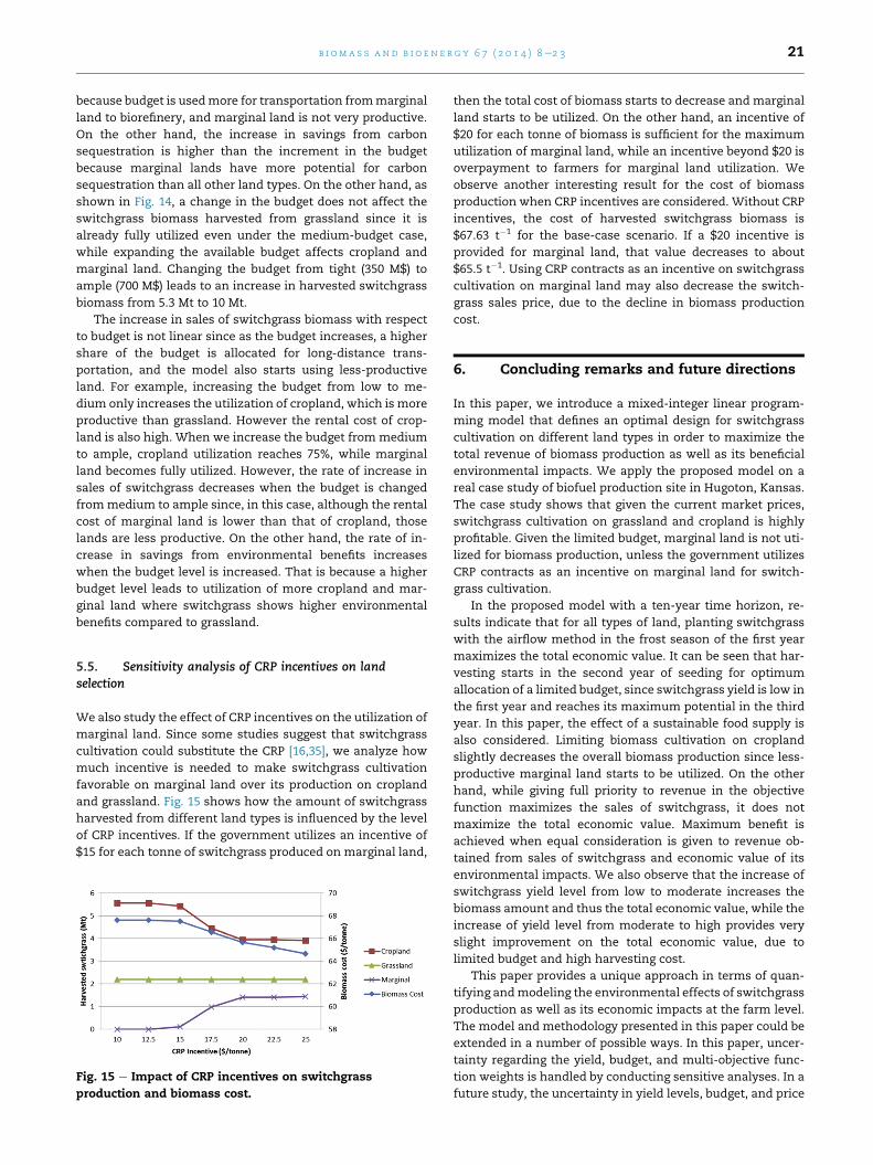
Fig. 6 displays profitability ratios in the base case for

various economical values obtained from switchgrass pro-

duction. The profitability ratio is obtained by dividing net

economical values (profits) of corresponding outputs by the

budget value in the base case. Total economic benefits

represent the summation of nominal values of switchgrass

sales, savings via carbon sequestration, and soil erosion pre-

vention. On the other hand, the objective function value is the

amount of economical values after the terms in the objective

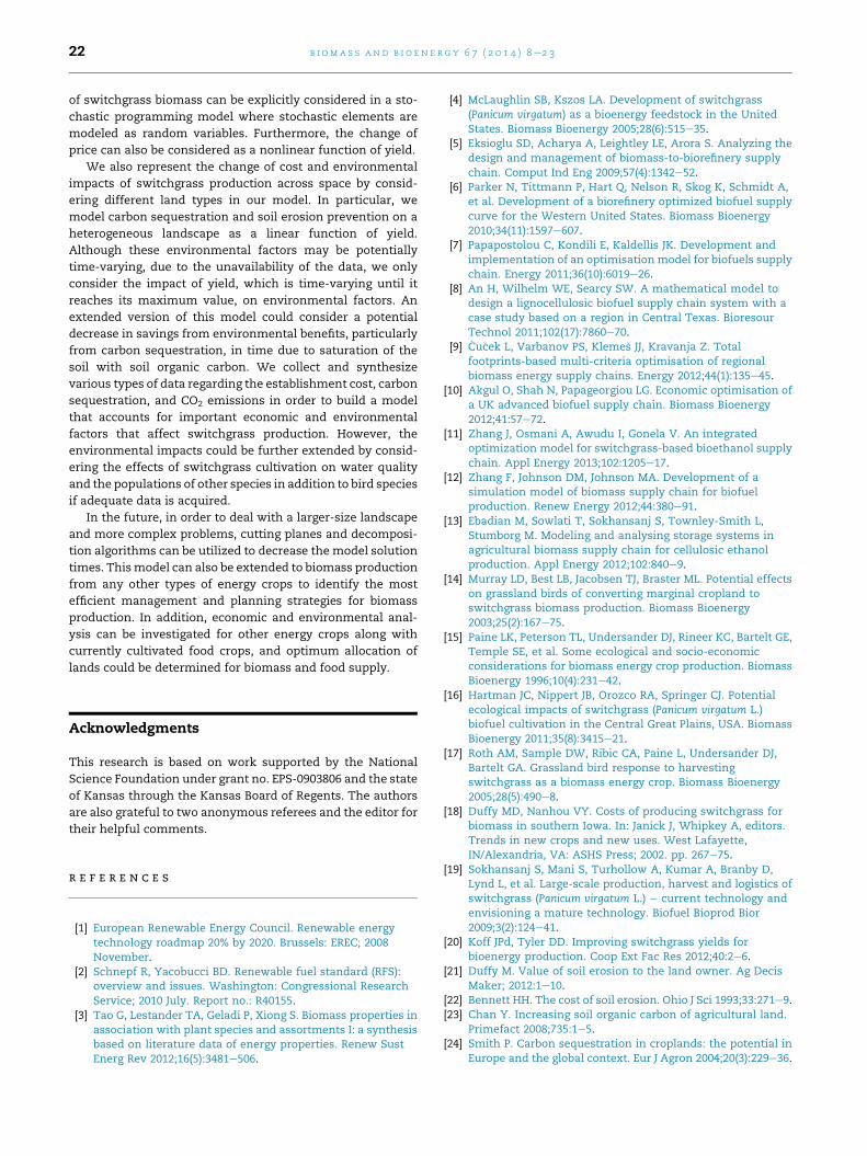
Fig. 4 e Optimal cost breakdown for the base-case scenario.

function aremultiplied with their corresponding weights. The

highest profitability ratio for total economic benefits is ob-

tained when equal consideration is given to both economic

and environmental factors.

In the following sections, we provide some scenario ana-

lyses by changing different parameter values in order to gain

better insight into the nature of the problem. First, we inves-

tigate the impact of different objective functionweights on the

results. The second analysis addresses the effect of changing

switchgrass yield levels on the model outputs. Third, we

perform another analysis in order to determine the impact of

sustainability factor on the solution, andfinally,we investigate

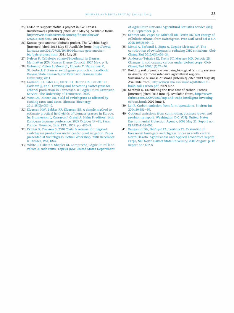
Fig. 7 e Economic value obtained from three objectives

based on changing weights.

b i om a s s a n d b i o e n e r g y 6 7 ( 2 0 1 4 ) 8e2 3 19

the impact of different budget levels. The values used in these

analyses are summarized in Table 5. Furthermore, we also

conduct a separate sensitivity analysis that examines the ef-

fect of CRP incentives on the selection of marginal land.

Fig. 9 e Economic value obtained from different objectives

based on changing yield levels.

5.1. Analysis of objective function weights

Three different weight cases are investigated to understand

the impact of objective functions on the results. For the first

set of weights (1 0 0), priority is given to revenue from biomass

sales, which emphasize the problem only from the farm

owner point of view. On the other hand, the second set of

weights (0.33 0.33 0.33) gives equal consideration to revenue

and environmental consequences of biomass production,

which may reflect the government’s goals. The last set of

weight (0 0.5 0.5) gives full consideration to the environment.

The total economic value obtained from the sales of

switchgrass, and savings from soil erosion and carbon

sequestration for three different objective function weights is

given in Fig. 7. The amount of switchgrass grown and har-

vested on different land types is also given for three different

objective function weights in Fig. 8. As shown in Figs. 7 and 8,

giving full consideration to the environment decreases the

amount of switchgrass harvested to zero, which results in no

sales. The equal-weight case (0.33 0.33 0.33) gives higher total

economic value than that in the profit priority case (1 0 0),

although the harvested amount decreases from 7.76 Mt to

7.30Mt. This is because in the equal-weight case, savings from

soil erosion and carbon sequestration increase faster than the

decrease in sales of switchgrass on marginal land. In this case

cropland, grassland, and marginal land account for 50%, 13%,

and 37%, respectively, of the overall biomass production.

Giving equal consideration to the environment and sales of

switchgrass, some production is shifted from grassland to

marginal land since marginal land has ten and two times

better savings for carbon sequestration and soil erosion,

respectively, than the savings from grassland. However, by

further emphasizing environmental benefits, the model uses

the entire harvesting budget to have almost 100%utilization of

all land types including grassland. However, in this case, the

change in soil erosion is minimal since switchgrass soil

erosion prevention is not high for grassland, and further uti-

lization of grassland does not provide much more additional

benefit.

Fig. 8 e Switchgrass yield and harvested amount based on

changing weights.

5.2. Analysis of switchgrass yield levels

In this study, potential switchgrass yield is assumed to be

mostly dependent on land types and establishment year.

However, lower and upper bounds are set on the potential

switchgrass yield in order to reflect the impact of various

factors such as changing weather conditions on potential

yield. Potential yield in low level is set to 33% less than that in

a moderate yield level, as shown in Table 1. Similarly, the

potential yield in high level is taken as 33%more than that in a

moderate yield level.

Figs. 9 and 10 show the effect of different yield levels on the

economic value and harvested switchgrass from different

land types, respectively. In the low-yield level case, all land

types are utilized for biomass harvesting since there is not

enough biomass grown on cropland and grassland. On the

other hand, increasing the potential yield level to a moderate

level removes marginal land from the solution. In other

words, amoderate biomass amount in cropland and grassland

leads to savings from the transportation cost, which can be

used for more harvesting. Removing less-productive marginal

lands from the solution leads to a higher economic value

because the total biomass amount increases from 6.23 Mt to

7.76Mt. However, further increasing the potential switchgrass

yield provides only a slight improvement in the sales of

switchgrass because, in this case, budget becomes a limiting

factor. We still obtain a slight increase in sales because the

same amount of biomass can be obtained from a closer region

Fig. 10 e Harvested yield from different land types based

on changing yield levels.

Fig. 11 e Economic value from three objective functions

based on sustainability factor.Fig. 13 e Economic value obtained from different objectives

based on changing budget.

b i om a s s a n d b i o e n e r g y 6 7 ( 2 0 1 4 ) 8e2 320

to the facility, which results in some savings from the trans-

portation cost and leads to more harvesting. Another inter-

esting result is obtained regarding savings from carbon

sequestration. A higher potential yield level decreases the

savings from carbon sequestration since the model does not

select marginal land, which leads to ten times more carbon

sequestration than that of grassland.

5.3. Analysis of sustainability factor

Figs. 11 and 12 provide the effect of the sustainability factor on

economic value obtained for different objective functions and

the amount of harvested switchgrass from different land

types, respectively. First, full availability of cropland for

biomass production is defined by setting the sustainability

factor to 0%. Then it has been increased to 25%. Finally, for full

security of the food supply, the sustainability factor has been

increased to 50%. Based on Figs. 11 and 12, there is no differ-

ence in results for sustainability factors of 0% and 25%, while

we observe a slight decrease in economic value from the sales

of switchgrass when the sustainability factor is set to 50%.

Since utilization of cropland is already less than 75% in the

base case, i.e., the sustainability constraint is not binding,

changing the sustainability factor from 0% to 25% (i.e., limiting

the usage of cropland for biomass production to 75%) does not

affect the results. The binding constraint on cropland

Fig. 12 e Harvested switchgrass based on sustainability

factor.

utilization is the budget constraint. On the other hand, when

we further increase the sustainability factor to 50% (i.e.,

limiting the usage of cropland to 50%), the model cannot use

the same amount of cropland as in the base case. Therefore, in

this case, the budget usage is shifted to marginal lands, which

are not so productive, leading to a decrease in the harvested

switchgrass biomass from 7.76 Mt to 7.50 Mt. By changing the

allocation of land types between the cases of 0% and 50%

sustainability factors, one can conclude that food supply

safety can be provided without losing too much economic

value.

5.4. Analysis of changing budget levels

We also investigate the effect of a changing budget on the

results. The economic value and harvested switchgrass

biomass are given in Figs. 13 and 14, respectively. Here, an

ample budget represents a sufficient budget amount for

seeding and harvesting on all types of land. A moderate

budget is set to 75% of the ample budget, while a tight budget

is considered to be 50% of the ample budget. Fig. 13 shows that

an increase in the budget results in an increase in all objective

functions in terms of economic value. However, the incre-

ment in sales in switchgrass biomass and savings from soil

erosion is slower than the increment in the budget. This is

Fig. 14 e Harvested yield from different land types based

on changing budget.

b i om a s s a n d b i o e n e r g y 6 7 ( 2 0 1 4 ) 8e2 3 21

because budget is usedmore for transportation frommarginal

land to biorefinery, and marginal land is not very productive.

On the other hand, the increase in savings from carbon

sequestration is higher than the increment in the budget

because marginal lands have more potential for carbon

sequestration than all other land types. On the other hand, as

shown in Fig. 14, a change in the budget does not affect the

switchgrass biomass harvested from grassland since it is

already fully utilized even under the medium-budget case,

while expanding the available budget affects cropland and

marginal land. Changing the budget from tight (350 M$) to

ample (700 M$) leads to an increase in harvested switchgrass

biomass from 5.3 Mt to 10 Mt.

The increase in sales of switchgrass biomass with respect

to budget is not linear since as the budget increases, a higher

share of the budget is allocated for long-distance trans-

portation, and the model also starts using less-productive

land. For example, increasing the budget from low to me-

dium only increases the utilization of cropland, which is more

productive than grassland. However the rental cost of crop-

land is also high. When we increase the budget from medium

to ample, cropland utilization reaches 75%, while marginal

land becomes fully utilized. However, the rate of increase in

sales of switchgrass decreases when the budget is changed

frommedium to ample since, in this case, although the rental

cost of marginal land is lower than that of cropland, those

lands are less productive. On the other hand, the rate of in-

crease in savings from environmental benefits increases

when the budget level is increased. That is because a higher

budget level leads to utilization of more cropland and mar-

ginal land where switchgrass shows higher environmental

benefits compared to grassland.

5.5. Sensitivity analysis of CRP incentives on landselection

We also study the effect of CRP incentives on the utilization of

marginal land. Since some studies suggest that switchgrass

cultivation could substitute the CRP [16,35], we analyze how

much incentive is needed to make switchgrass cultivation

favorable on marginal land over its production on cropland

and grassland. Fig. 15 shows how the amount of switchgrass

harvested from different land types is influenced by the level

of CRP incentives. If the government utilizes an incentive of

$15 for each tonne of switchgrass produced on marginal land,

Fig. 15 e Impact of CRP incentives on switchgrass

production and biomass cost.

then the total cost of biomass starts to decrease and marginal

land starts to be utilized. On the other hand, an incentive of

$20 for each tonne of biomass is sufficient for the maximum

utilization of marginal land, while an incentive beyond $20 is

overpayment to farmers for marginal land utilization. We

observe another interesting result for the cost of biomass

production when CRP incentives are considered. Without CRP

incentives, the cost of harvested switchgrass biomass is

$67.63 t�1 for the base-case scenario. If a $20 incentive is

provided for marginal land, that value decreases to about

$65.5 t�1. Using CRP contracts as an incentive on switchgrass

cultivation on marginal land may also decrease the switch-

grass sales price, due to the decline in biomass production

cost.

6. Concluding remarks and future directions

In this paper, we introduce a mixed-integer linear program-

ming model that defines an optimal design for switchgrass

cultivation on different land types in order to maximize the

total revenue of biomass production as well as its beneficial

environmental impacts. We apply the proposed model on a

real case study of biofuel production site in Hugoton, Kansas.

The case study shows that given the current market prices,

switchgrass cultivation on grassland and cropland is highly

profitable. Given the limited budget, marginal land is not uti-

lized for biomass production, unless the government utilizes

CRP contracts as an incentive on marginal land for switch-

grass cultivation.

In the proposed model with a ten-year time horizon, re-

sults indicate that for all types of land, planting switchgrass

with the airflow method in the frost season of the first year

maximizes the total economic value. It can be seen that har-

vesting starts in the second year of seeding for optimum

allocation of a limited budget, since switchgrass yield is low in

the first year and reaches its maximum potential in the third

year. In this paper, the effect of a sustainable food supply is

also considered. Limiting biomass cultivation on cropland

slightly decreases the overall biomass production since less-

productive marginal land starts to be utilized. On the other

hand, while giving full priority to revenue in the objective

function maximizes the sales of switchgrass, it does not

maximize the total economic value. Maximum benefit is

achieved when equal consideration is given to revenue ob-

tained from sales of switchgrass and economic value of its

environmental impacts. We also observe that the increase of

switchgrass yield level from low to moderate increases the

biomass amount and thus the total economic value, while the

increase of yield level from moderate to high provides very

slight improvement on the total economic value, due to

limited budget and high harvesting cost.

This paper provides a unique approach in terms of quan-

tifying andmodeling the environmental effects of switchgrass

production as well as its economic impacts at the farm level.

The model and methodology presented in this paper could be

extended in a number of possible ways. In this paper, uncer-

tainty regarding the yield, budget, and multi-objective func-

tion weights is handled by conducting sensitive analyses. In a

future study, the uncertainty in yield levels, budget, and price

b i om a s s a n d b i o e n e r g y 6 7 ( 2 0 1 4 ) 8e2 322

of switchgrass biomass can be explicitly considered in a sto-

chastic programming model where stochastic elements are

modeled as random variables. Furthermore, the change of

price can also be considered as a nonlinear function of yield.

We also represent the change of cost and environmental

impacts of switchgrass production across space by consid-

ering different land types in our model. In particular, we

model carbon sequestration and soil erosion prevention on a

heterogeneous landscape as a linear function of yield.

Although these environmental factors may be potentially

time-varying, due to the unavailability of the data, we only

consider the impact of yield, which is time-varying until it

reaches its maximum value, on environmental factors. An

extended version of this model could consider a potential

decrease in savings from environmental benefits, particularly

from carbon sequestration, in time due to saturation of the

soil with soil organic carbon. We collect and synthesize

various types of data regarding the establishment cost, carbon

sequestration, and CO2 emissions in order to build a model

that accounts for important economic and environmental

factors that affect switchgrass production. However, the

environmental impacts could be further extended by consid-

ering the effects of switchgrass cultivation on water quality

and the populations of other species in addition to bird species

if adequate data is acquired.

In the future, in order to deal with a larger-size landscape

and more complex problems, cutting planes and decomposi-

tion algorithms can be utilized to decrease the model solution

times. Thismodel can also be extended to biomass production

from any other types of energy crops to identify the most

efficient management and planning strategies for biomass

production. In addition, economic and environmental anal-

ysis can be investigated for other energy crops along with

currently cultivated food crops, and optimum allocation of

lands could be determined for biomass and food supply.

Acknowledgments

This research is based on work supported by the National

Science Foundation under grant no. EPS-0903806 and the state

of Kansas through the Kansas Board of Regents. The authors

are also grateful to two anonymous referees and the editor for

their helpful comments.

r e f e r e n c e s

[1] European Renewable Energy Council. Renewable energytechnology roadmap 20% by 2020. Brussels: EREC; 2008November.

[2] Schnepf R, Yacobucci BD. Renewable fuel standard (RFS):overview and issues. Washington: Congressional ResearchService; 2010 July. Report no.: R40155.

[3] Tao G, Lestander TA, Geladi P, Xiong S. Biomass properties inassociation with plant species and assortments I: a synthesisbased on literature data of energy properties. Renew SustEnerg Rev 2012;16(5):3481e506.

[4] McLaughlin SB, Kszos LA. Development of switchgrass(Panicum virgatum) as a bioenergy feedstock in the UnitedStates. Biomass Bioenergy 2005;28(6):515e35.

[5] Eksioglu SD, Acharya A, Leightley LE, Arora S. Analyzing thedesign and management of biomass-to-biorefinery supplychain. Comput Ind Eng 2009;57(4):1342e52.

[6] Parker N, Tittmann P, Hart Q, Nelson R, Skog K, Schmidt A,et al. Development of a biorefinery optimized biofuel supplycurve for the Western United States. Biomass Bioenergy2010;34(11):1597e607.

[7] Papapostolou C, Kondili E, Kaldellis JK. Development andimplementation of an optimisation model for biofuels supplychain. Energy 2011;36(10):6019e26.

[8] An H, Wilhelm WE, Searcy SW. A mathematical model todesign a lignocellulosic biofuel supply chain system with acase study based on a region in Central Texas. BioresourTechnol 2011;102(17):7860e70.

[9] �Cu�cek L, Varbanov PS, Kleme�s JJ, Kravanja Z. Totalfootprints-based multi-criteria optimisation of regionalbiomass energy supply chains. Energy 2012;44(1):135e45.

[10] Akgul O, Shah N, Papageorgiou LG. Economic optimisation ofa UK advanced biofuel supply chain. Biomass Bioenergy2012;41:57e72.

[11] Zhang J, Osmani A, Awudu I, Gonela V. An integratedoptimization model for switchgrass-based bioethanol supplychain. Appl Energy 2013;102:1205e17.

[12] Zhang F, Johnson DM, Johnson MA. Development of asimulation model of biomass supply chain for biofuelproduction. Renew Energy 2012;44:380e91.

[13] Ebadian M, Sowlati T, Sokhansanj S, Townley-Smith L,Stumborg M. Modeling and analysing storage systems inagricultural biomass supply chain for cellulosic ethanolproduction. Appl Energy 2012;102:840e9.

[14] Murray LD, Best LB, Jacobsen TJ, Braster ML. Potential effectson grassland birds of converting marginal cropland toswitchgrass biomass production. Biomass Bioenergy2003;25(2):167e75.

[15] Paine LK, Peterson TL, Undersander DJ, Rineer KC, Bartelt GE,Temple SE, et al. Some ecological and socio-economicconsiderations for biomass energy crop production. BiomassBioenergy 1996;10(4):231e42.

[16] Hartman JC, Nippert JB, Orozco RA, Springer CJ. Potentialecological impacts of switchgrass (Panicum virgatum L.)biofuel cultivation in the Central Great Plains, USA. BiomassBioenergy 2011;35(8):3415e21.

[17] Roth AM, Sample DW, Ribic CA, Paine L, Undersander DJ,Bartelt GA. Grassland bird response to harvestingswitchgrass as a biomass energy crop. Biomass Bioenergy2005;28(5):490e8.

[18] Duffy MD, Nanhou VY. Costs of producing switchgrass forbiomass in southern Iowa. In: Janick J, Whipkey A, editors.Trends in new crops and new uses. West Lafayette,IN/Alexandria, VA: ASHS Press; 2002. pp. 267e75.

[19] Sokhansanj S, Mani S, Turhollow A, Kumar A, Branby D,Lynd L, et al. Large-scale production, harvest and logistics ofswitchgrass (Panicum virgatum L.) e current technology andenvisioning a mature technology. Biofuel Bioprod Bior2009;3(2):124e41.

[20] Koff JPd, Tyler DD. Improving switchgrass yields forbioenergy production. Coop Ext Fac Res 2012;40:2e6.

[21] Duffy M. Value of soil erosion to the land owner. Ag DecisMaker; 2012:1e10.

[22] Bennett HH. The cost of soil erosion. Ohio J Sci 1993;33:271e9.[23] Chan Y. Increasing soil organic carbon of agricultural land.

Primefact 2008;735:1e5.[24] Smith P. Carbon sequestration in croplands: the potential in

Europe and the global context. Eur J Agron 2004;20(3):229e36.

b i om a s s a n d b i o e n e r g y 6 7 ( 2 0 1 4 ) 8e2 3 23

[25] USDA to support biofuels project in SW Kansas.Businessweek [Internet] [cited 2013 May 5]. Available from:,http://www.businessweek.com/ap/financialnews/D9OO2T880.htm; 2011 July 27.

[26] Kansas gets another biofuels project. The Wichita Eagle[Internet] [cited 2013 May 5]. Available from:, http://www.kansas.com/2011/07/26/1948944/kansas-gets-another-biofuels-project.html; 2011 July 26.

[27] Nelson R. Cellulosic ethanol/bioethanol in Kansas.Manhattan (KS): Kansas Energy Council; 2007 May. p. 8.

[28] Holman J, Gillen R, Moyer JL, Roberts T, Harmoney K,Sloderbeck P. Kansas switchgrass production handbook.Kansas State Research and Extension: Kansas StateUniversity; 2011.

[29] Garland CD, Bates GE, Clark CD, Dalton DA, Gerloff DC,Goddard JJ, et al. Growing and harvesting switchgrass forethanol production in Tennessee. UT Agricultural ExtensionService: The University of Tennessee; 2008.

[30] West DR, Kincer DR. Yield of switchgrass as affected byseeding rates and dates. Biomass Bioenergy2011;35(9):4057e9.

[31] Elbersen HW, Bakker RR, Elbersen BS. A simple method toestimate practical field yields of biomass grasses in Europe.In: Sjunnesson L, Carrasco J, Grassi A, Helm P, editors. 14thEuropean biomass conference, 2005 October 17e21, Paris,France. Florence, Italy: ETA; 2005. pp. 476e9.

[32] Painter K, Fransen S. 2010 Costs & returns for irrigatedswitchgrass production under center pivot irrigation. Paperpresented at Switchgrass Biofuel Workshop; 2010 December8. Prosser, WA, USA.

[33] White R, Habets S, Shepler GL, Lamprecht J. Agricultural landvalues & cash rents. Topeka (KS): United States Department

of Agriculture National Agricultural Statistics Service (KS);2011 September. p. 4.

[34] Schmer MR, Vogel KP, Mitchell RB, Perrin RK. Net energy ofcellulosic ethanol from switchgrass. Proc Natl Acad Sci U S A2008;105(2):464e9.

[35] Monti A, Barbanti L, Zatta A, Zegada-Lizarazu W. Thecontribution of switchgrass in reducing GHG emissions. GlobChang Biol 2012;4(4):420e34.

[36] Anderson-Teixeira KJ, Davis SC, Masters MD, Delucia EH.Changes in soil organic carbon under biofuel crops. GlobChang Biol 2009;1(1):75e96.

[37] Building soil organic carbon using biological farming systemsin Australia’s more intensive agricultural regions.Sustainable Business Australia [Internet] [cited 2013 May 20].Available from:, http://www.sba.asn.au/sba/pdf/BioCCS-build-soil-carbon.pdf; 2009 June.

[38] Serchuk D. Calculating the true cost of carbon. Forbes[Internet] [cited 2013 June 2]. Available from:, http://www.forbes.com/2009/06/03/cap-and-trade-intelligent-investing-carbon.html; 2009 June 3.

[39] Lal R. Carbon emission from farm operations. Environ Int2004;30:981e90.

[40] Optional emissions from commuting, business travel andproduct transport. Washington D.C. (US): United StatesEnvironmental Protection Agency; 2008 May 21. Report no.:EPA430-R-08-006.

[41] Bangsund DA, DeVuyst EA, Leistritz FL. Evaluation ofbreakeven farm-gate switchgrass prices in south centralNorth Dakota. Agribusiness and Applied Economics Report.Fargo, ND: North Dakota State University; 2008 August. p. 12.Report no.: 632-S.