Optim EngDOI 10.1007/s11081-013-9226-6

A mixed-integer nonlinear program for the optimaldesign and dispatch of distributed generation systems

Kristopher A. Pruitt · Sven Leyffer ·Alexandra M. Newman · Robert J. Braun

Received: 6 January 2012 / Accepted: 22 June 2013© Springer Science+Business Media New York 2013

Abstract Maturing distributed generation (DG) technologies have promoted inter-est in alternative sources of energy for commercial building applications due to theirpotential to supply on-site heat and power at a lower cost and emissions rate com-pared to centralized generation. Accordingly, we present an optimization model thatdetermines the mix, capacity, and operational schedule of DG technologies that min-imize economic and environmental costs subject to the heat and power demands of abuilding and to the performance characteristics of the technologies. The technologiesavailable to design the system include lead-acid batteries, photovoltaic cells, solid ox-ide fuel cells, heat exchangers, and a hot water storage tank. Modeling the acquisitionand operation of discrete technologies requires integer restrictions, and modeling thevariable electric efficiency of the fuel cells and the variable temperature of the tankwater introduces nonlinear equality constraints. Thus, our optimization model is anonconvex, mixed-integer nonlinear programming (MINLP) problem. Given the dif-ficulties associated with solving large, nonconvex MINLPs to global optimality, wepresent convex underestimation and linearization techniques to bound and solve theproblem. The solutions provided by our techniques are close to those provided by ex-isting MINLP solvers for small problem instances. However, our methodology offers

K.A. Pruitt · A.M. Newman (B)Division of Economics and Business, Colorado School of Mines, Golden, CO 80401, USAe-mail: anewman@mines.edu

K.A. Pruitte-mail: kpruitt@mines.edu

S. LeyfferMathematics and Computer Science Division, Argonne National Laboratory, Argonne, IL 60439,USAe-mail: leyffer@mcs.anl.gov

R.J. BraunDepartment of Mechanical Engineering, Colorado School of Mines, Golden, CO 80401, USAe-mail: rbraun@mines.edu

K.A. Pruitt et al.

the possibility to solve large problem instances that exceed the capacity of existingsolvers and that are critical to the real-world application of the model.

Keywords Global optimization · Mixed-integer nonlinear programming ·Distributed generation · Combined heat and power

1 Introduction

Distributed generation (DG) has gained interest as an alternative source of powerfor new and existing buildings in the residential, commercial, and industrial sectors.Rather than solely purchasing electricity from a centralized utility, a building ownercan invest in an on-site system to supply power using non-renewable technologiessuch as reciprocating engines, microturbines, and fuel cells, and renewable technolo-gies such as photovoltaic (PV) cells and wind turbines. When integrated with heatexchangers, solar thermal collectors, and absorption chillers, on-site systems can alsomeet some of the building heating and cooling demands. In addition to generation,DG systems can include electric and thermal storage technologies to address the un-certainty in the supply available from renewable generators or to take advantage oftime periods in which utility prices are low. Our research considers the integration oftechnologies such as these with existing commercial buildings.

There are a number of reasons why DG systems should be considered for commer-cial building applications. Between 2005 and 2009, the commercial sector accountedfor 36 % of electricity consumption across all sectors, which resulted in an averageannual cost of roughly $127 billion (see EIA 2011b). Gumerman et al. (2003) listbenefits to the owner of DG systems, which have the potential to reduce this eco-nomic burden. These benefits include a lower cost of electricity (in some markets),protection from utility price volatility, more reliable power, and greater energy effi-ciency. The authors further describe potential benefits of DG to the local community.When composed of “clean” natural gas-fed or renewable technologies, DG systemsemit less carbon dioxide than most centralized power plants. Smaller, on-site gener-ation also addresses much of the opposition in local communities to the constructionof large power plants and transmission lines. Yet, based on Department of Energyprojections for electricity consumption and DG market penetration, on-site systemswill supply a mere 2 % of commercial sector electricity demand in 2035 (see EIA2011a).

This disparity between the noted operational benefits of DG systems and the mod-est prediction for future market penetration exists for a variety of reasons. From apurely economic standpoint, many power utilities maintain low prices for electricitywhile the capital costs for DG technologies remain high. This discrepancy has dis-couraged building owners from investing in DG systems. However, due to their loweremissions rates compared to centralized power plants, some DG technologies affordlower environmental costs which building owners often have no economic incentiveto internalize. Properly considering all of the costs associated with generation, whichinclude environmental costs and other externalities, effectively increases the priceof electricity from the utility and may make DG more economically viable. Finally,

Distributed generation system design and dispatch

DG has experienced limited implementation simply due to a lack of understandingregarding how to design (i.e., configure and size) and dispatch (i.e., operate) suchmixed-resource systems. The objective of our research is to address this lack of un-derstanding with an optimization model that determines how to design and dispatcha DG system at minimum economic and environmental cost.

Previous research regarding DG focuses on various aspects of the optimal systemdesign and dispatch. Many studies address the optimal performance of an individualDG technology, but do not resolve the system-level design and dispatch problem ofintegrating, sizing, and operating multiple technologies. Other research seeks the op-timal dispatch of an existing system, but does not consider the optimal system design.Our research focuses on the optimal design and dispatch of a DG system. Similarlyfocused research in the literature applies simulation models, evolutionary algorithms(EAs), or more traditional mathematical programming algorithms, such as branch-and-bound, to the design and dispatch problem (e.g., Georgilakis 2006; Burer et al.2003; Weber et al. 2006; Siddiqui et al. 2005a). In general, studies that apply simu-lation or EAs cannot guarantee the global optimality of their solutions. The existingapplications of branch-and-bound to the design and dispatch problem provide theguarantee of global optimality, but fail to consider many of the detailed performancecharacteristics of the technologies that are required to realistically model the systemoperation. Our research contributes to the literature by providing techniques for deter-mining the provably globally minimum cost DG system design and dispatch withoutsacrificing realistic operation of the technologies.

Modeling the operation of such a complex system requires constraints to controlthe operational status (i.e., on or off), capacity, ramping (i.e., increasing or decreas-ing power output), and variable efficiency of the generators, as well as constraintsto control the state-of-charge (i.e., inventory) of electric storage technologies and thetemperature of thermal storage technologies. These constraints can include integervariables in each time period, connections between consecutive time periods, andnonlinear equalities. Given all of these characteristics, the resulting model is a large,nonseparable, nonconvex, mixed-integer, nonlinear programming (MINLP) problem.The algorithms suitable for solving large, nonconvex MINLPs are limited and de-pendent on the problem structure. The application of a nonlinear branch-and-boundalgorithm requires methods to obtain global upper and lower bounds on the objec-tive value at each node in order to converge to the optimal solution. However, thesebounds can be difficult to obtain for large, nonconvex problems. Thus, we developproblem-specific convex underestimation techniques, motivated by our engineeringinsight, to obtain global lower bounds on the objective value of our MINLP. We alsodevelop a linearization heuristic to obtain integer-feasible solutions, and thus globalupper bounds, for our MINLP. These bounding techniques can be applied as part ofa nonlinear branch-and-bound algorithm to solve large instances of the DG systemdesign and dispatch problem to global optimality.

The remainder of this paper is organized as follows: Sect. 2 presents the formu-lation of the MINLP. In Sect. 3, we discuss the problem structure, the convex un-derestimation of the MINLP, and our linearization heuristic. Section 4 compares thesolutions provided by our techniques with those provided by existing solvers. Finally,Sect. 5 concludes.

K.A. Pruitt et al.

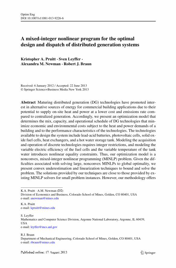
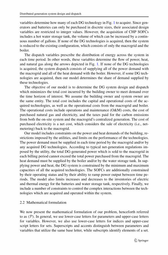
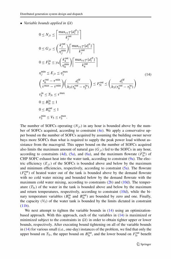
Fig. 1 Combined heat and power (CHP), distributed generation (DG) system consisting of photovoltaic(PV) cells, power-only and CHP solid-oxide fuel cells (SOFCs), lead-acid batteries, and a hot water storagetank

2 Model

The specific system addressed in this research is depicted in Fig. 1. We consider theretrofit of an existing commercial building with a combined heat and power (CHP),DG system. Prior to DG acquisition, the building receives electricity from the powerutility (i.e., macrogrid) and heat from a natural gas-fired boiler. The cooling demandis met by existing vapor-compression air conditioning units and is included as partof the power demand. The heat demand includes space and water heating, both ofwhich are met with hot water (i.e., space heat is provided by hot water radiators).The DG system being considered for acquisition generates power with fixed-tilt PVcells and/or natural gas-fed solid oxide fuel cells (SOFCs) which, according to Greeneand Hammerschlag (2000), provide lower carbon emissions than other DG-scale gen-erators. The CHP SOFCs are integrated with heat exchangers and a water tank, whichallow for the storage of thermal energy in the form of hot water. The system also in-cludes the option for electric storage using lead-acid batteries. We do not considerother non-renewable generators, wind turbines, solar thermal, or absorption chillers.However, our model can be adapted to include these technologies. Next, we providea general description of the system model, followed by the detailed mathematicalformulation.

2.1 Model description

Our model includes parameters for the time fidelity and horizon being considered,the heat and power demands of the building, the pricing and carbon emissions ratesof the utilities, and the capital and operational costs, carbon emissions rates, and per-formance characteristics of all the technologies in the system. All of these parametersare treated as deterministic.

The model includes two types of variables: design and dispatch. The design vari-ables establish the configuration and capacity of the DG system. In other words, these

Distributed generation system design and dispatch

variables determine how many of each DG technology in Fig. 1 to acquire. Since gen-erators and batteries can only be purchased in discrete sizes, their associated designvariables are restricted to integer values. However, the acquisition of CHP SOFCsincludes a hot water storage tank, the volume of which can be increased by a contin-uous number of gallons. If none of the DG technologies is acquired, then the systemis reduced to the existing configuration, which consists of only the macrogrid and theboiler.

The dispatch variables prescribe the distribution of energy across the system ineach time period. In other words, these variables determine the flow of power, heat,and natural gas along the arrows depicted in Fig. 1. If none of the DG technologiesis acquired, the system dispatch consists of supplying all of the power demand withthe macrogrid and all of the heat demand with the boiler. However, if some DG tech-nologies are acquired, then our model determines the share of demand supplied bythese technologies.

The objective of our model is to determine the DG system design and dispatchwhich minimizes the total cost incurred by the building owner to meet demand overthe time horizon of interest. We assume the building owner and system owner arethe same entity. The total cost includes the capital and operational costs of the ac-quired technologies, as well as the operational costs from the macrogrid and boiler.The operational costs include operations and maintenance (O&M) costs, the cost ofpurchased natural gas and electricity, and the taxes paid for the carbon emissionsfrom both the on-site system and the macrogrid’s centralized generation. The cost ofpurchased electricity is a net cost, which considers the sale of electricity (i.e., net-metering) back to the macrogrid.

Our model includes constraints on the power and heat demands of the building, re-strictions imposed by the utilities, and limits on the performance of the technologies.The power demand must be supplied in each time period by the macrogrid and/or byany acquired DG technologies. According to typical net-generation regulations im-posed by the utility, the total DG-generated power which is sold to the macrogrid ineach billing period cannot exceed the total power purchased from the macrogrid. Theheat demand must be supplied by the boiler and/or by the water storage tank. In sup-plying power and heat, the DG system is constrained by the minimum and maximumcapacities of all the acquired technologies. The SOFCs are additionally constrainedby their operating status and by their ability to ramp power output between time pe-riods. The model also limits increases and decreases to the inventories of electricand thermal energy for the batteries and water storage tank, respectively. Finally, weinclude a number of constraints to control the complex interactions between the tech-nologies which are acquired and operated within the system.

2.2 Mathematical formulation

We now present the mathematical formulation of our problem, henceforth referredto as (P). In general, we use lower-case letters for parameters and upper-case lettersfor variables. However, we also use lower-case letters for indices and upper-casescript letters for sets. Superscripts and accents distinguish between parameters andvariables that utilize the same base letter, while subscripts identify elements of a set.

K.A. Pruitt et al.

Some parameters and variables are only defined for certain set elements, which arelisted in each definition. The units of each parameter and variable are provided inbrackets after its definition. Throughout the definitions, “technology” is abbreviatedas “tech.”, “average” is abbreviated as “avg.”, and “respectively” is abbreviated as“resp.”

• Setsn ∈N : set of all monthst ∈ Tn: set of all hours in month n (T = ⋃

n Tn)i ∈ I: set of all cost elementsj ∈ J : set of all techs.Note: To avoid verbosity, we define the elements of J numerically as 1 = Bat-tery, 2 = PV, 3 = Power SOFC, 4 = CHP SOFC, 5 = Storage Tank, 6 = Boiler.

• Time and demand parametersδ = demand time increment [hours]dPt , dH

t = avg. power and heat demand, resp., in hour t [kW]• Cost and emissions parameters

cj = amortized capital cost of each tech. j = 1, . . . ,5 [$/kWh, $/kW, or $/gal]mj = avg. O&M cost of each tech. j = 2,3,4,6 [$/kWh]pt , gt = price of power and gas, resp., from the utility in hour t [$/kWh]pmax

n = peak demand price of power from the utility in month n [$/kW/month]z = tax on carbon emissions [$/kg]zp, zg = avg. carbon emissions rate for power and gas, resp. [kg/kWh]

• Power generation and storage parameterskoutj , kin

j = power rating out of and into, resp., each tech. j = 1, . . . ,4 [kW]

smaxj , smin

j = max and min, resp., storage capacity of tech. j = 1 [kWh]ajt = avg. availability of tech. j = 2 based on weather in hour t [fraction]μj = max turn-down (i.e., min power output) of each tech. j = 3,4 [fraction]σj = start-up time for each tech. j = 3,4 to reach μj [hours]r

upj , rdown

j = max ramp-up and down rate, resp., for each tech. j = 3,4 [kW/hr]

ηmaxj , ηmin

j = max and min, resp., electric efficiency of each tech. j = 1,3,4[fraction]

• Heat generation and storage parametersvmaxj , vmin

j = max and min, resp., storage capacity of tech. j = 5 [gallons]ηj = avg. thermal efficiency of each tech. j = 5,6 [fraction]αj = mean ambient heat loss of water stored in tech. j = 5 [fraction]γj = avg. exhaust gas output from tech. j = 4 per natural gas input [kg/kWh]hj = specific heat of fluid output from each tech. j = 4,5 [kWh/(kg °C) orkWh/(gal °C)]τ outj , τ in

j = avg. fluid temperature out of and into, resp., each tech. j = 4,5,6[°C]τmax, τmin = max and min, resp., temperature of water in the system [°C]

• System design variablesCi = total cost of cost element i over the time horizon [$]Aj = number of each tech. j = 1, . . . ,5 acquired [integer]Vj = water storage capacity of tech. j = 5 [gallons]

Distributed generation system design and dispatch

• Power dispatch and storage variablesUout

t ,U int = power purchased from and sold to the utility, resp., in hour t [kW]

Umaxn = max power purchased from the utility in month n [kW]

P outj t = aggregate power output from each tech. j = 1, . . . ,4 in hour t [kW]

P inj t = aggregate power input to tech. j = 1 in hour t [kW]

Sjt = aggregate state-of-charge of tech. j = 1 at the start of hour t [kWh]Njt = number of each tech. j = 3,4 operating in hour t [integer]Njt = increased number of each tech. j = 3,4 operating from t −1 to t [integer]Ejt = electric efficiency of each tech. j = 3,4 operating in hour t [fraction]

• Heat dispatch and storage variablesGjt = aggregate natural gas input to each tech. j = 3,4,6 in hour t [kW]F out

j t = flowrate of water out of tech. j = 5 in hour t [gal/hr]

F inj t = flowrate of exhaust gas into tech. j = 5 in hour t [kg/hr]

Tjt = temperature of water stored in technology j = 5 in hour t [°C]B in

j t = 1 if water in tech. j = 5 is above (τ in5 + ε) in hour t , 0 otherwise [binary]

Boutj t = 1 if water in tech. j = 5 is above τ out

6 in hour t , 0 otherwise [binary]• Problem (P)

(see Sect. 2.3.1—Minimum total cost)Minimize

∑

i∈ICi (1)

subject to(see Sect. 2.3.2—Power and heat demand)

(ηmax

1 P out1t − P in

1t

) +∑

j=2..4

P outj t + (

Uoutt − U in

t

) = dPt ∀t ∈ T (2a)

h5(τ out

6 − τ in5

)F out

5t

[(

1 −[

1 − τ out6 − τmin

T5t − τmin

]

Bout5t

)−1]

= dHt ∀t ∈ T (2b)

(see Sect. 2.3.3—Utility restrictions)

Umaxn ≥ Uout

t ∀n ∈N , t ∈ Tn (3a)∑

t∈Tn

U int ≤

∑

t∈Tn

Uoutt ∀n ∈N (3b)

(see Sect. 2.3.4—Power capacity)

P out1t ≤ kout

1 A1 ∀t ∈ T (4a)

P in1t ≤ kin

1 A1 ∀t ∈ T (4b)

P out2t ≤ a2t k

out2 A2 ∀t ∈ T (4c)

μjkoutj Njt ≤ P out

j t ≤ koutj Njt ∀j = 3,4, t ∈ T (4d)

Njt ≤ Aj ∀j = 3,4, t ∈ T (4e)

K.A. Pruitt et al.

(see Sect. 2.3.5—Electric efficiency)

Ejt =(

ηmaxj − μjη

minj

1 − μj

)

−(

ηmaxj − ηmin

j

koutj (1 − μj )

)(P out

j t

Njt

)

∀j = 3,4, t ∈ T (5a)

(see Sect. 2.3.6—Natural gas consumption)

Gjt = P outj t

Ejt

∀j = 3,4, t ∈ T (6a)

G6t = h5Fout5t (τ out

6 − T5t )(1 − Bout5t )

η6∀t ∈ T (6b)

(see Sect. 2.3.7—Start up and ramping)

Nj,t+1 − Njt ≤ Nj,t+1 ∀j = 3,4, t < |T | (7a)

−δrdownj Njt ≤ P out

j,t+1 − P outj t ≤ δr

upj Nj,t+1 ∀j = 3,4, t < |T | (7b)

(see Sect. 2.3.8—Power storage)

S1,t+1 − S1t = δ(ηmax

1 P in1t − P out

1t

) ∀t < |T | (8a)

smin1 A1 ≤ S1t ≤ smax

1 A1 ∀t ∈ T (8b)

S1,1 = S1,|T | (8c)

(see Sect. 2.3.9—Heat capacity)

F in5t ≤ γ4G4t ∀t ∈ T (9a)

(see Sect. 2.3.10—Heat storage)

T5,t+1 − (1 − α5B

in5t

)T5t

= δη5h4Fin5t (τ

out4 − T5t ) − δh5F

out5t (T5t − τ in

5 )

h5V5∀t < |T | (10a)

T5t − τ in5 ≤ (

τmax − τ in5

)A5 ∀t ∈ T (10b)

εB in5t ≤ T5t − τ in

5 ≤ ε + (τmax − τ in

5 − ε)B in

5t ∀t ∈ T (10c)(τ in

5 − τ out6

)(1 − Bout

5t

) ≤ T5t − τ out6 ≤ (

τmax − τ out6

)Bout

5t ∀t ∈ T (10d)

T5,1 = T5,|T | (10e)

(see Sect. 2.3.11—Heat storage acquisition)

A5 ≤ A4 ≤⌈

maxt∈T {dPt }

kout4

⌉

A5 (11a)

vmin5 ≤ V5 ≤ vmax

5 (11b)

Distributed generation system design and dispatch

(see Sect. 2.3.12—Non-negativity and integrality)

P outj t ,P in

j t , Sjt , Nj t ,Ejt ,Gjt ,Foutj t ,F in

j t , Tjt , Vj ≥ 0 ∀j ∈ J , t ∈ T (12a)

Uoutt ,U in

t ,Umaxn ≥ 0 ∀n ∈N , t ∈ T (12b)

Aj ,Njt ≥ 0, integer ∀j �= 5, t ∈ T (12c)

Aj ,Binj t ,B

outj t , binary, ∀j = 5, t ∈ T (12d)

2.3 Detailed discussion of formulation

Next, we discuss the objective function and constraints of (P) in more detail.

2.3.1 Minimum total cost

The objective is to minimize the total cost over the entire time horizon. The totalcost expressed in the objective function (1) includes the capital and operational costsof the acquired technologies, as well as the existing operational costs resulting fromdemand met by the macrogrid and boiler.

The fixed capital cost, C1, consists of the total amortized cost of all the DG tech-nologies that are acquired:

C1 = c1smax1 A1 +

∑

j=2..4

cj koutj Aj + c5

(V5 − vmin

5

).

The capital cost of the CHP SOFCs is greater than that of the power-only SOFCs inorder to account for the acquisition of the water storage tank and heat exchangers.The water tank’s initial size (vmin

5 ) is based on the building heating load. However,the tank size can be increased for an additional cost per gallon.

The initial capital cost for each of the technologies can be amortized in a number ofdifferent ways. One method of amortization uses the parameters and general equationthat follow:

ρ = interest rate [% (fraction) per time horizon]λj = average lifetime of technology j [number of time horizons]κj = initial capital cost of technology j [$/kWh, $ /kW, or $/gal]

cj = κj eρλj

λj

. (13)

The numerator of Eq. (13) calculates what κj is eventually worth after investment atinterest rate ρ over the average lifetime λj of technology j (see Nicholson and Snyder2008). Thus, the numerator represents the lifetime opportunity cost of acquiring thetechnology rather than investing the initial capital cost at the current rate of return.The lifetime opportunity cost is then divided by λj to determine the opportunity costper time horizon, which we call the amortized capital cost cj . Ultimately, the primaryfocus of this research is not on the method of amortization. Rather, the final amortized

K.A. Pruitt et al.

cost (cj ) is the value of interest. Equation (13) is just one method for calculating thatcost, without loss of generality.

The variable operational costs of the DG system consist of O&M costs for the PVcells and SOFCs, the cost of natural gas to fuel the SOFCs, the cost of the carbonemissions associated with the combustion of natural gas, and the negative cost (i.e.,revenue) from the sale of power to the macrogrid. The O&M costs, C2, for the PVcells and SOFCs increase with the energy output:

C2 =∑

j=2..4,t

mj δPoutj t .

The O&M cost for the CHP SOFCs is greater than that for the power-only SOFCsto account for the additional operational costs of the water tank and heat exchangers.Due to the limited need for variable maintenance on lead-acid battery systems, theO&M costs for the batteries are assumed fixed and are treated as part of the capitalcost. The parameter δ is included to appropriately convert units of power (kW) tounits of energy (kWh).

Fuel and emissions costs, C3, are incurred both to start up the SOFCs (i.e., toreach operating temperature) and to operate them within their performance limits.These costs depend on the price (gt ) of natural gas from the local utility, the price(zzg) of carbon emissions, as determined by the tax rate and the emissions rate, andthe total amount of gas required for start up and operation:

C3 =∑

j=3..4,t

(gt + zzg

)[σjμjkj

2ηminj

Nj t + δGjt

]

.

Our formulation assumes a carbon tax exists where the building is located and thatthe tax is paid by the building owner. We further assume that the SOFCs consumenatural gas with the same fixed electric efficiency during start up as at maximumpower output. Thus, the amount of gas required for a single SOFC to reach operatingtemperature is treated as a fixed value. The variable Njt determines how many SOFCsstart up in a given time period, which allows for the calculation of the total amount ofgas required. Once an SOFC reaches operating temperature, the amount of natural gas(Gjt ) consumed depends on the power output and the electric efficiency as definedin constraint (6a).

The final operational cost for the DG technologies is the negative cost, C4, associ-ated with the sale of power to the macrogrid:

C4 = −∑

t

pt δUint .

We assume that net-metering is available with the local power utility and that theutility can purchase power from the building owner in any hour at the prevailingmarket rate. However, the total power purchased by the utility in each billing cycle issubject to the restrictions imposed by constraint (3b).

In addition to the capital and operational costs of the acquired DG technologies,the system incurs the cost of electricity purchased from the macrogrid and the opera-tional costs for the boiler. If DG technologies are not acquired, then the macrogrid and

Distributed generation system design and dispatch

boiler costs are the only costs. The macrogrid charges both hourly and peak monthlyrates, which determine the total electricity cost, C5:

C5 =∑

t

(pt + zzp

)δUout

t +∑

n

pmaxn Umax

n .

Depending on the rate schedule dictated by the power utility for the building andlocation of interest, the charges pt and pmax

n could vary by time-of-day and/or sea-son. We must also consider the cost of the carbon emitted by the generation sourcesemployed by the macrogrid. Our formulation applies an average carbon emissionsrate (zp) for all of the macrogrid’s generation sources and assumes that the buildingowner is taxed for the emissions associated with the purchased electricity. For bothnatural gas and power utilities, the fixed monthly customer charge for service is notincluded in the formulation since this cost is constant and therefore does not impactthe optimal solution.

Finally, the total cost includes the O&M, fuel, and emissions costs, C6, for theexisting boiler:

C6 =∑

t

(η6m6 + gt + zzg

)δG6t .

Similar to the SOFCs, the fuel and emissions costs depend on the price of naturalgas and the price of carbon emissions. In contrast to the SOFCs, the average ther-mal efficiency (η6) of the boiler is treated as fixed. The amount of natural gas (G6t )consumed depends on whether the temperature of the water flowing to the boiler isabove or below the required delivery temperature. The relationship between the wa-ter temperature and the amount of natural gas consumed by the boiler is defined inconstraint (6b).

2.3.2 Power and heat demand

Constraint (2a) ensures that the hourly demand for power is met by the net dischargeof the batteries (after accounting for the discharge efficiency ηmax

1 ), the PV cells, thepower-only and CHP SOFCs, and the net supply from the macrogrid. Constraint (2b)dictates that the hourly demand for heat must be met by a mix of hot and cold waterflow. The demanded hot water, which is heated by the CHP SOFC exhaust and/or bythe boiler, must be delivered at a fixed temperature (τ out

6 ). If the temperature of the hotwater is above delivery temperature (i.e., Bout

5t = 1), then the hot water must be mixedwith cold water at the minimum system temperature (τmin). As the temperature ofthe tank water increases, the required flow of cold water for mixing increases, andthe required flow of hot water from the tank decreases.

2.3.3 Utility restrictions

Constraint (3a) establishes the peak power load supplied by the macrogrid in eachmonthly billing cycle as the largest hourly load supplied by the macrogrid eachmonth. Constraint (3b) dictates that the DG system cannot be a “net-generator” of

K.A. Pruitt et al.

power in each monthly billing cycle. Accordingly, the total power sold to the macro-grid each month cannot exceed the total power purchased from the macrogrid eachmonth.

2.3.4 Power capacity

Constraints (4a) and (4b) limit the rate at which power is discharged from and chargedto, respectively, all of the acquired batteries. If batteries are not acquired, then thecharge and discharge rates are set equal to zero. Constraint (4c) ensures that only afraction (a2t ) of the nameplate power capacity of the acquired PV cells is availablein each hour, based on the prevailing weather conditions. Because the solar radiationis often low enough that the available power from PV cells is zero (e.g., during thenight), there is no minimum power output enforced for PV cells. Constraint (4d)limits the maximum and minimum power output of all operating SOFCs in a givenhour. The maximum turn-down (μj ) results from the minimum operating temperaturenecessary for the SOFCs to produce power. Constraint (4e) dictates that the number ofSOFCs operating in a given hour cannot exceed the number acquired. Power suppliedby the macrogrid in each hour is unconstrained in this formulation.

2.3.5 Electric efficiency

Constraint (5a) demonstrates that the average electric efficiency across all SOFCs isa function of the number (Njt ) of SOFCs operating and the total power (P out

j t ) theyproduce. Our formulation assumes that each operating SOFC provides an equal shareof the total power produced in a given hour. Using the maximum (ηmax

j ) and minimum

(ηminj ) electric efficiencies as endpoints, we treat the average electric efficiency of all

SOFCs as a decreasing linear function of the share of total power provided by a singleSOFC.

2.3.6 Natural gas consumption

Constraint (6a) dictates that the total amount of natural gas consumed by all of theoperating power-only or CHP SOFCs in each hour is the quotient of their total poweroutput and their average electric efficiency. Constraint (6b) calculates the amount ofnatural gas consumed by the boiler in each hour as the quotient of its heat output andits average thermal efficiency. The amount of heat the boiler must provide dependson the temperature (T5t ) of the water from the storage tank, if one is acquired. Weassume the hot water must be delivered to the building’s faucets and radiators ata fixed temperature (τ out

6 ). If the temperature of the water from the storage tank isbelow τ out

6 in a given hour (i.e., Bout5t = 0), then the boiler must provide the additional

heat to increase the water temperature to τ out6 . In this case, the amount of heat is

calculated as the product of the specific heat of the tank water (h5), the flowrate ofthe tank water (F out

5t ), and the difference (τ out6 −T5t ) between the delivery temperature

and the tank water temperature. If the temperature of the water from the storage tankis at or above τ out

6 in a given hour (i.e., Bout5t = 1), then no additional heating from

the boiler is required. If a storage tank is not acquired, then the boiler must provideall of the heat demand, which entails heating all of the water from the average returntemperature (τ in

5 ) up to delivery temperature (τ out6 ).

Distributed generation system design and dispatch

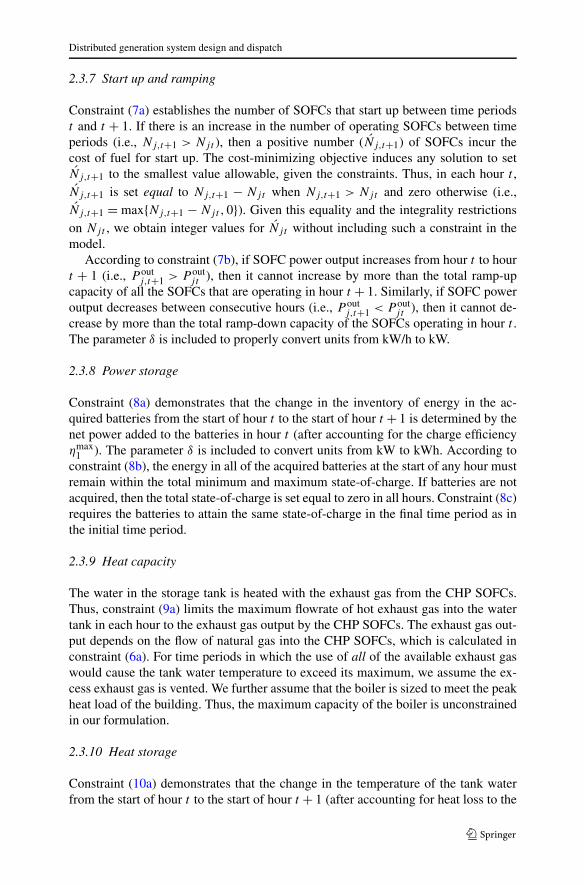
2.3.7 Start up and ramping

Constraint (7a) establishes the number of SOFCs that start up between time periodst and t + 1. If there is an increase in the number of operating SOFCs between timeperiods (i.e., Nj,t+1 > Njt ), then a positive number (Nj,t+1) of SOFCs incur thecost of fuel for start up. The cost-minimizing objective induces any solution to setNj,t+1 to the smallest value allowable, given the constraints. Thus, in each hour t ,Nj,t+1 is set equal to Nj,t+1 − Njt when Nj,t+1 > Njt and zero otherwise (i.e.,Nj,t+1 = max{Nj,t+1 − Njt ,0}). Given this equality and the integrality restrictionson Njt , we obtain integer values for Njt without including such a constraint in themodel.

According to constraint (7b), if SOFC power output increases from hour t to hourt + 1 (i.e., P out

j,t+1 > P outj t ), then it cannot increase by more than the total ramp-up

capacity of all the SOFCs that are operating in hour t + 1. Similarly, if SOFC poweroutput decreases between consecutive hours (i.e., P out

j,t+1 < P outj t ), then it cannot de-

crease by more than the total ramp-down capacity of the SOFCs operating in hour t .The parameter δ is included to properly convert units from kW/h to kW.

2.3.8 Power storage

Constraint (8a) demonstrates that the change in the inventory of energy in the ac-quired batteries from the start of hour t to the start of hour t + 1 is determined by thenet power added to the batteries in hour t (after accounting for the charge efficiencyηmax

1 ). The parameter δ is included to convert units from kW to kWh. According toconstraint (8b), the energy in all of the acquired batteries at the start of any hour mustremain within the total minimum and maximum state-of-charge. If batteries are notacquired, then the total state-of-charge is set equal to zero in all hours. Constraint (8c)requires the batteries to attain the same state-of-charge in the final time period as inthe initial time period.

2.3.9 Heat capacity

The water in the storage tank is heated with the exhaust gas from the CHP SOFCs.Thus, constraint (9a) limits the maximum flowrate of hot exhaust gas into the watertank in each hour to the exhaust gas output by the CHP SOFCs. The exhaust gas out-put depends on the flow of natural gas into the CHP SOFCs, which is calculated inconstraint (6a). For time periods in which the use of all of the available exhaust gaswould cause the tank water temperature to exceed its maximum, we assume the ex-cess exhaust gas is vented. We further assume that the boiler is sized to meet the peakheat load of the building. Thus, the maximum capacity of the boiler is unconstrainedin our formulation.

2.3.10 Heat storage

Constraint (10a) demonstrates that the change in the temperature of the tank waterfrom the start of hour t to the start of hour t + 1 (after accounting for heat loss to the

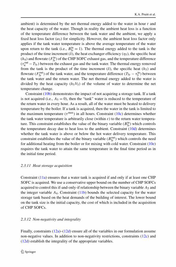
K.A. Pruitt et al.

ambient) is determined by the net thermal energy added to the water in hour t andthe heat capacity of the water. Though in reality the ambient heat loss is a functionof the temperature difference between the tank water and the ambient, we apply afixed heat loss factor (α5) for simplicity. However, the ambient heat loss factor onlyapplies if the tank water temperature is above the average temperature of the waterupon return to the tank (i.e., B in

5t = 1). The thermal energy added to the tank is theproduct of the time increment (δ), the heat exchanger efficiency (η5), the specific heat(h4) and flowrate (F in

5t ) of the CHP SOFC exhaust gas, and the temperature difference(τ out

4 −T5t ) between the exhaust gas and the tank water. The thermal energy removedfrom the tank is the product of the time increment (δ), the specific heat (h5) andflowrate (F out

5t ) of the tank water, and the temperature difference (T5t − τ in5 ) between

the tank water and the return water. The net thermal energy added to the water isdivided by the heat capacity (h5V5) of the volume of water to determine the nettemperature change.

Constraint (10b) demonstrates the impact of not acquiring a storage tank. If a tankis not acquired (i.e., A5 = 0), then the “tank” water is reduced to the temperature ofthe return water in every hour. As a result, all of the water must be heated to deliverytemperature by the boiler. If a tank is acquired, then the water in the tank is limited tothe maximum temperature (τmax) in all hours. Constraint (10c) determines whetherthe tank water temperature is arbitrarily close (within ε) to the return water tempera-ture. This constraint establishes the value of the binary variable (B in

5t ) which controlsthe temperature decay due to heat loss to the ambient. Constraint (10d) determineswhether the tank water is above or below the hot water delivery temperature. Thisconstraint establishes the value of the binary variable (Bout

5t ) which controls the needfor additional heating from the boiler or for mixing with cold water. Constraint (10e)requires the tank water to attain the same temperature in the final time period as inthe initial time period.

2.3.11 Heat storage acquisition

Constraint (11a) ensures that a water tank is acquired if and only if at least one CHPSOFC is acquired. We use a conservative upper bound on the number of CHP SOFCsacquired to control this if-and-only-if relationship between the binary variable A5 andthe integer variable A4. Constraint (11b) bounds the selected capacity for the waterstorage tank based on the heat demands of the building of interest. The lower boundon the tank size is the initial capacity, the cost of which is included in the acquisitionof CHP SOFCs.

2.3.12 Non-negativity and integrality

Finally, constraints (12a)–(12d) ensure all of the variables in our formulation assumenon-negative values. In addition to non-negativity restrictions, constraints (12c) and(12d) establish the integrality of the appropriate variables.

Distributed generation system design and dispatch

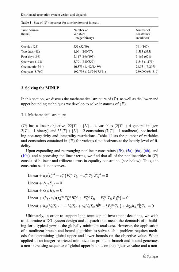
Table 1 Size of (P) instances for time horizons of interest

Time horizon(hours)

Number ofvariables(integer/binary)

Number ofconstraints(nonlinear)

One day (24) 533 (52/49) 791 (167)

Two days (48) 1,061 (100/97) 1,583 (335)

Four days (96) 2,117 (196/193) 3,167 (671)

One week (168) 3,701 (340/337) 5,543 (1,175)

One month (744) 16,373 (1,492/1,489) 24,551 (5,207)

One year (8,760) 192,736 (17,524/17,521) 289,090 (61,319)

3 Solving the MINLP

In this section, we discuss the mathematical structure of (P), as well as the lower andupper bounding techniques we develop to solve instances of (P).

3.1 Mathematical structure

(P) has a linear objective, 22|T | + |N | + 4 variables (2|T | + 4 general integer,2|T | + 1 binary), and 33|T | + |N | − 2 constraints (7|T | − 1 nonlinear), not includ-ing non-negativity and integrality restrictions. Table 1 lists the number of variablesand constraints contained in (P) for various time horizons at the hourly level of fi-delity.

Upon expanding and rearranging nonlinear constraints (2b), (5a), (6a), (6b), and(10a), and suppressing the linear terms, we find that all of the nonlinearities in (P)

consist of bilinear and trilinear terms in equality constraints (see below). Thus, theconstraint set is nonconvex.

Linear + h5(τ out

6 − τ in5

)F out

5t T5t + dHt T5tB

out5t = 0

Linear + NjtEjt = 0

Linear + GjtEjt = 0

Linear + (h5/η6)(τ out

6 F out5t Bout

5t + F out5t T5t − F out

5t T5tBout5t

) = 0

Linear + h5(V5T5,t+1 − V5T5t + α5V5T5tB

in5t + δF out

5t T5t

) + δη5h4Fin5t T5t = 0

Ultimately, in order to support long-term capital investment decisions, we wishto determine a DG system design and dispatch that meets the demands of a build-ing for a typical year at the globally minimum total cost. However, the applicationof a nonlinear branch-and-bound algorithm to solve such a problem requires meth-ods for determining global upper and lower bounds on the objective value. Whenapplied to an integer-restricted minimization problem, branch-and-bound generatesa non-increasing sequence of global upper bounds on the objective value and a non-

K.A. Pruitt et al.

decreasing sequence of global lower bounds on the objective value which eventuallyconverge (within some tolerance) to provide the optimal solution. In general, globalupper bounds are provided by integer-feasible solutions obtained with local solversand global lower bounds are provided by solutions to continuous relaxations of theinteger problem. Both types of bounds can be difficult to obtain for large, nonconvexMINLPs. Our testing indicates few existing MINLP solvers are capable of findingsolutions to one-day instances of (P), and none of those tested can provide solutionsfor time horizons greater than one week. Additionally, the nonconvex nature of (P)

dictates that solutions to continuous relaxations do not necessarily provide globallower bounds. Accordingly, the next two sections discuss our techniques to obtainlower and upper bounds which can be applied in a nonlinear branch-and-bound algo-rithm.

3.2 Lower bounding: convex underestimation

A lower bound for a mixed-integer linear programming (MILP) minimization prob-lem is obtained by relaxing the integrality restrictions and solving the resulting con-tinuous problem. A lower bound for an MINLP minimization problem can also beobtained in this manner as long as the problem is convex. However, nonconvex prob-lems provide no guarantee of obtaining a global lower bound when solving the NLPrelaxation. Thus, we formulate a convex underestimation problem, henceforth re-ferred to as (U), to obtain a global lower bound on (P).

Convex underestimation methods similar to those suggested by McCormick(1976) are still applied in the literature today. Indeed, this classical idea has beenadapted for use in some state-of-the-art software (Sahinidis 1996), and results havebeen reported in Tawarmalani and Sahinidis (2003) and Bao et al. (2009). Accord-ing to Eqs. (3) and (4) of Adjiman and Floudas (2008), bilinear and trilinear terms,respectively, are underestimated by their convex envelope. The convex envelopesare constructed by replacing each of the nonlinear terms with a new variable andadding linear inequality constraints that bound the new variable. Bilinear terms re-quire four constraints on the new variable while trilinear terms require eight con-straints. Considering some of our nonlinear terms are repeated across constraints,(P) contains 9|T | − 1 distinct bilinear terms and 2|T | − 1 distinct trilinear termsthat must be replaced with new variables. Accordingly, the (U) formulation is iden-tical to (P) with the exceptions of adding 11|T | − 2 new continuous variables,replacing each of the bilinear and trilinear terms with the appropriate new con-tinuous variable, and adding 52|T | − 12 new linear constraints. Hence, (U) is anMILP, the solution to which provides a global lower bound on the optimal solutionto (P).

The formulation of the convex envelopes in (U) requires the following upperand lower bounds on each of the original variables in the bilinear and trilinearterms:

Distributed generation system design and dispatch

• Variable bounds applied in (U)

0 ≤ Njt ≤⌈

maxt∈T {dPt }

koutj

⌉

0 ≤ Gjt ≤(

koutj

ηminj

)⌈maxt∈T {dP

t }koutj

⌉

0 ≤ F in5t ≤ γ4

(kout

4

ηmin4

)⌈maxt∈T {dP

t }kout

4

⌉

ηminj ≤ Ejt ≤ ηmax

j

(τ out

6 − τmin

τmax − τmin

)(dHt

h5(τout6 − τ in

5 )

)

≤ F out5t ≤

(dHt

h5(τout6 − τ in

5 )

)

τ in5 ≤ T5t ≤ τmax

0 ≤ B in5t ≤ 1

0 ≤ Bout5t ≤ 1

vmin5 ≤ V5 ≤ vmax

5 .

(14)

The number of SOFCs operating (Njt ) in any hour is bounded above by the num-ber of SOFCs acquired, according to constraint (4e). We apply a conservative up-per bound on the number of SOFCs acquired by assuming the building owner neverbuys more SOFCs than what is required to supply the peak power load without as-sistance from the macrogrid. This upper bound on the number of SOFCs acquiredalso limits the maximum amount of natural gas (Gjt ) fed to the SOFCs in any hour,according to constraints (4d), (5a), and (6a), and the maximum flowrate (F in

5t ) ofCHP SOFC exhaust heat into the water tank, according to constraint (9a). The elec-tric efficiency (Ejt ) of the SOFCs is bounded above and below by the maximumand minimum efficiencies, respectively, according to constraint (5a). The flowrate(F out

5t ) of heated water out of the tank is bounded above by the demand flowratewith no cold water mixing and bounded below by the demand flowrate with themaximum cold water mixing, according to constraints (2b) and (10d). The temper-ature (T5t ) of the water in the tank is bounded above and below by the maximumand return temperatures, respectively, according to constraint (10d), while the bi-nary temperature variables (B in

5t and Bout5t ) are bounded by zero and one. Finally,

the capacity (V5) of the water tank is bounded by the limits dictated in constraint(11b).

We next attempt to tighten the variable bounds in (14) using an optimization-based approach. With this approach, each of the variables in (14) is maximized orminimized subject to the constraints in (U) in order to obtain tighter upper or lowerbounds, respectively. After executing bound tightening on all of the variable boundsin (14) for various small (i.e., one-day) instances of the problem, we find that only theupper bound on T5t , the upper bound on Bout

5t , and the lower bound on F out5t benefit

K.A. Pruitt et al.

from the bound tightening. The fact that these three bounds can be tightened logicallyfollows from the relationships dictated by constraints (2b), (10a), and (10d). In certaintime periods, the maximum possible inflow of heat from the CHP SOFCs and theminimum required outflow of heat to meet demand could make it impossible forthe tank water temperature (T5t ) to reach its upper bound (τmax), or even deliverytemperature (τ out

6 ), in the following time period, according to constraint (10a). If thetank water temperature is below the delivery temperature, then the indicator variable(Bout

5t ) must be set to its lower bound (zero), according to constraint (10d), and theflow of hot water (F out

5t ) must be set to its upper bound, according to constraint (2b).Based on this information, we expedite the bound tightening procedure for larger (i.e.,two-day and greater) instances of the problem by only applying the optimization tothe upper bound on T5t (referred to as T5t ) and subsequently directly calculating thenew upper bound on Bout

5t (referred to as Bout5t ) and the new lower bound on F out

5t

(referred to as F out5t ). To further speed the bound tightening, we relax integrality in

(U) as part of the following algorithm:

• Bound tightening algorithm

1. Set T5t = τmax, Bout5t = 1, F out

5t = (τ out

6 −τmin

τmax−τmin )(dHt

h5(τout6 −τ in

5 )) ∀t .

2. Loop ∀t ∈ T .(a) Maximize T5t subject to (U) with integrality relaxed.(b) Set T5t equal to the objective value resulting from (a).(c) Set Bout

5t = 1 if T5t > τ out6 and 0 otherwise.

(d) Set F out5t = (1 − [1 − τ out

6 −τmin

T5t−τmin ]Bout5t )(

dHt

h5(τout6 −τ in

5 )).

This algorithm can be repeated multiple times to try and achieve even tighterbounds. However, empirical evidence suggests the majority of the improvement inthe bounds occurs within the first two to three repetitions. We also find that the algo-rithm results in the greatest improvement in the bounds on T5t ,B

out5t , and F out

5t in hoursthat follow large spikes in the heat demand. These tighter bounds are then applied in(U), with the original objective function and integrality once again enforced, to ob-tain an improved (i.e., greater) global lower bound on the optimal objective value for(P). For the instances presented in Sect. 4, the bound tightening algorithm increasesthe global lower bound on (P) by an average of 1.6 %. We next present techniquesfor obtaining a global upper bound on the optimal objective value for (P).

3.3 Upper bounding: linearization heuristic

An upper bound for an MI(N)LP minimization problem is provided by any integer-feasible solution. One integer-feasible solution to (P) is to acquire no DG technolo-gies and meet all of the building’s demand with the macrogrid and boiler. The costof this “no DG” solution can be directly calculated, without solving (P), using theC5 and C6 portions of the objective function and setting Uout

t = dPt ∀t,Umax

n =maxt∈Tn

{dPt } ∀n, and G6t = dH

t /η6 ∀t . However, the “no DG” solution providesa weak upper bound on the total cost for the optimal solution to (P) if DG technolo-gies are economically viable. Thus, we wish to find an integer-feasible solution, if

Distributed generation system design and dispatch

one exists, that includes some DG technologies and provides a lower total cost, andthus a tighter upper bound, than the “no DG” solution. Integer-feasible solutions canbe obtained by solving (P) with existing MINLP solvers for small problem instances.However, based on our testing, larger problem instances (i.e., greater than one week)cannot be solved with the currently available solvers. Accordingly, we next present alinearization heuristic, henceforth referred to as (H), for determining integer-feasiblesolutions to (P) that can be applied to the large instances.

The intuition behind (H) is the observation that fixing the electric efficiency of theSOFCs (E3t ,E4t ) and the tank water temperature (T5t ) renders (P) linear. Simplermodels in the literature similarly fix the efficiencies of generators and fix, or ignore,the temperature of thermal storage devices to avoid nonlinearity (e.g., Siddiqui et al.2005b). When E3t and E4t are fixed, constraint (5a) is linearized by clearing the de-nominator on the right-hand side of the equation and constraint (6a) is linear withoutmodification. When T5t is fixed, constraints (10c) and (10d) fix the values of B in

5t

and Bout5t , respectively. With T5t ,B

in5t , and Bout

5t all fixed, constraints (2b) and (6b) arelinear without modification and constraint (10a) is linearized by clearing the denomi-nator on the right-hand side of the equation. Thus, the (H) formulation is identical to(P) with the exception of fixing 3|T | continuous variable values (E3t ,E4t , and T5t )and 2|T | binary variable values (B in

5t and Bout5t ). Consequently, any feasible solution

to the MILP (H) is feasible for the MINLP (P).Although we obtain (P)-feasible solutions from (H)-feasible solutions, the fixed

values for E3t ,E4t , T5t ,Bin5t , and Bout

5t must be carefully selected in order to achieve(H)-feasibility. Additionally, not every (P)-feasible solution produces a total cost lessthan the “no DG” solution. In general, the fixed variable values used in (H) will pro-duce lower cost (P)-feasible solutions if those fixed values are tailored to the powerand heat demands of the building of interest. Hence, we next present techniques forselecting the fixed variable values used in (H) with the goal of obtaining (P)-feasiblesolutions that incur a lower total cost than the “no DG” solution. In presenting thesetechniques, we distinguish between two types of system design solutions: DG sys-tems with only power generation and storage (referred to as “power DG”) and DGsystems with both power and heat generation and storage (referred to as “CHP DG”).Depending on the particular problem instance, one of these system design types mayproduce a lower cost solution than the other.

For a “power DG” system, the selection of fixed values for E4t , T5t ,Bin5t , and Bout

5t

is trivial. Because there is no SOFC exhaust heat capture in this case, CHP SOFCsare never acquired and the associated electric efficiency can simply be set to its min-imum. Also, because there is no water storage tank, the water enters the boiler atreturn temperature in every hour and must be fully heated to delivery temperature.Less trivial, however, is the selection of the fixed values for the power-only SOFCelectric efficiency (E3t ). One might ignore the specific power demands of the build-ing and simply fix the efficiency to the same value (e.g., the minimum, average, ormaximum efficiency) in all hours. However, this approach forces the SOFCs to oper-ate at the same power output for all hours in which they are utilized (see constraint(5a)) and, therefore, is unlikely to produce a (P)-feasible solution with a total cost aslow as that produced by efficiency values which are tailored to the power demands.We can obtain these tailored fixed values for E3t from the solution to (U ). Given the

K.A. Pruitt et al.

underestimation of constraint (5a) in (U ), we cannot directly apply the values for E3t

from the solution to (U ). However, the solution to (U ) provides valid values for P out3t

and N3t , referred to as P out3t and N3t , that we use along with constraint (5a) to derive

E3t . These tailored values are applied in (H) as part of the following algorithm toobtain a (P)-feasible solution:

• “Power DG” (P)-feasible solution algorithm

1. Solve (U) and store resulting values for P out3t and N3t ∀t .

2. Set T5t = τ in5 , B in

5t = 0, Bout5t = 0, and E4t = ηmin

4 ∀t .

3. Set E3t = E3t = (ηmax

3 −μ3ηmin3

1−μ3) − (

ηmax3 −ηmin

3kout

3 (1−μ3))(P out

3t /N3t ) if N3t > 0, ηmin3 other-

wise ∀t .4. Solve (H) and return its solution.

For “CHP DG” systems, the tailored fixed values for E3t and E4t are both deter-mined from the solution to (U ), as previously demonstrated for E3t with “Power DG”systems. However, it may no longer be advisable to trivially fix the values for T5t ,B

in5t ,

and Bout5t to their minima. Fixing these variables to their minimum values prevents the

storage of heat across time periods (see constraint (10a)) and likely wastes a large por-tion of the available exhaust heat from the CHP SOFCs. We would prefer to use asmuch of the exhaust heat as possible to keep the tank water as hot as possible and toreduce the heat provided by the boiler. Hence, the fixed values for T5t ,B

in5t , and Bout

5t

should be tailored to the heat supplied to the water tank by the CHP SOFCs and theheat demanded from the water tank by the building.

Any fixed values selected for T5t ,Bin5t , and Bout

5t must satisfy constraints (10a)through (10e) to be (H)-feasible. In order to derive fixed values for T5t that satisfyconstraint (10a), we require values for the flowrate of heat from the CHP SOFCs(F in

5t ), the flowrate of hot water from the tank (F out5t ), and the tank size (V5). The

values for F in5t and V5 are determined from the solution to (U ). Given P out

4t and E4t ,along with constraints (6a) and (9a), we calculate the maximum flowrate of exhaustgas from the CHP SOFCs in each hour and use this as the value for F in

5t . The value forV5 is taken directly from the solution to (U ). With a fixed inflow of heat and fixed tanksize, we can iteratively calculate values for T5t that satisfy constraint (10a), values forB in

5t that satisfy constraint (10c), and values for Bout5t that satisfy constraint (10d). As

part of the algorithm, we also calculate values for F out5t that satisfy constraint (2b);

however, these values are not fixed in (H). Finally, in order to ensure the satisfactionof constraint (10e), we set the tank temperature in the initial time period (T5,1) equalto the temperature in the terminal time period (T5,|T |) after the first execution of thealgorithm. We then continue executing the algorithm until the terminal tank temper-ature is equal to the initial tank temperature. Empirically, we find that the terminaltemperature is so insensitive to the initial temperature that only two repetitions totalof the algorithm are necessary. These tailored temperature values are applied in (H)

as part of the following algorithm to obtain a “CHP DG” (P)-feasible solution:

• “CHP DG” (P)-feasible solution algorithm

1. Solve (U) and store resulting values for P outj t , Nj t ∀j, t , and V5.

Distributed generation system design and dispatch

2. Set Ejt = Ej t ∀j, t , F in5t = γ4(P

out4t /E4t ) ∀t, V5 = V5, and T5,1 = τmax.

3. Loop ∀t ∈ T .(a) Set B in

5t = 1 if T5t > (τ in5 + ε), 0 otherwise.

(b) Set Bout5t = 1 if T5t > τ out

6 , 0 otherwise.

(c) Let F out5t = (1 − [1 − τ out

6 −τmin

T5t−τmin ]Bout5t )(

dHt

h5(τout6 −τ in

5 )).

(d) Set

T5,t+1 = max

{

τ in5 ,min

{

τmax,(1 − α5B

in5t

)T5t

+ δη5h4Fin5t (τ

out4 − T5t ) − δh5F

out5t (T5t − τ in

5 )

h5V5

}}

.

4. If T5,|T | = T5,1 then go to Step 5. Otherwise, set T5,1 = T5,|T | and return toStep 3.

5. Solve (H) and return its solution.

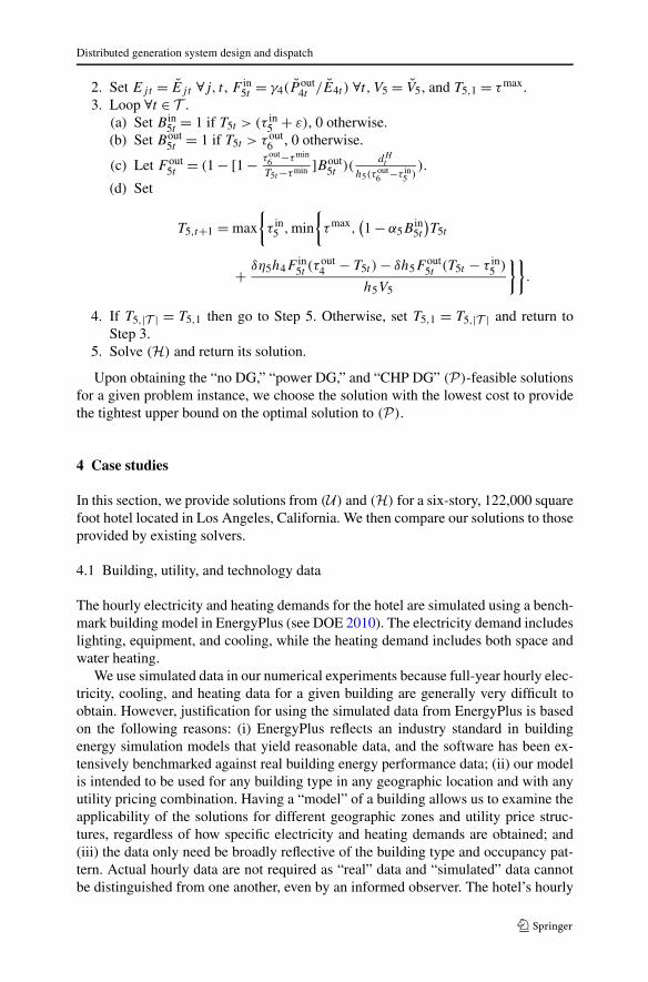
Upon obtaining the “no DG,” “power DG,” and “CHP DG” (P)-feasible solutionsfor a given problem instance, we choose the solution with the lowest cost to providethe tightest upper bound on the optimal solution to (P).

4 Case studies

In this section, we provide solutions from (U) and (H) for a six-story, 122,000 squarefoot hotel located in Los Angeles, California. We then compare our solutions to thoseprovided by existing solvers.

4.1 Building, utility, and technology data

The hourly electricity and heating demands for the hotel are simulated using a bench-mark building model in EnergyPlus (see DOE 2010). The electricity demand includeslighting, equipment, and cooling, while the heating demand includes both space andwater heating.

We use simulated data in our numerical experiments because full-year hourly elec-tricity, cooling, and heating data for a given building are generally very difficult toobtain. However, justification for using the simulated data from EnergyPlus is basedon the following reasons: (i) EnergyPlus reflects an industry standard in buildingenergy simulation models that yield reasonable data, and the software has been ex-tensively benchmarked against real building energy performance data; (ii) our modelis intended to be used for any building type in any geographic location and with anyutility pricing combination. Having a “model” of a building allows us to examine theapplicability of the solutions for different geographic zones and utility price struc-tures, regardless of how specific electricity and heating demands are obtained; and(iii) the data only need be broadly reflective of the building type and occupancy pat-tern. Actual hourly data are not required as “real” data and “simulated” data cannotbe distinguished from one another, even by an informed observer. The hotel’s hourly

K.A. Pruitt et al.

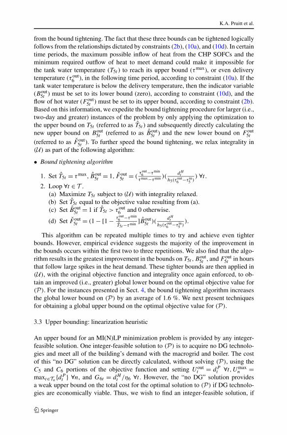
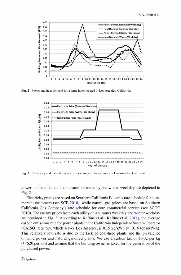
Fig. 2 Power and heat demand for a large hotel located in Los Angeles, California

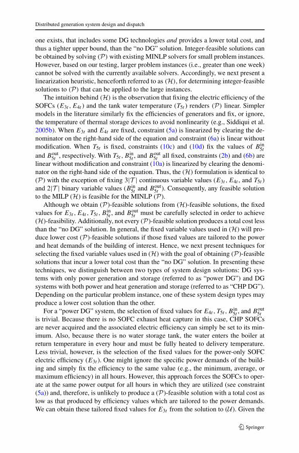
Fig. 3 Electricity and natural gas prices for commercial customers in Los Angeles, California

power and heat demands on a summer weekday and winter weekday are depicted inFig. 2.

Electricity prices are based on Southern California Edison’s rate schedule for com-mercial customers (see SCE 2010), while natural gas prices are based on SouthernCalifornia Gas Company’s rate schedule for core commercial service (see SCGC2010). The energy prices from each utility on a summer weekday and winter weekdayare provided in Fig. 3. According to Kaffine et al. (Kaffine et al. 2011), the averagecarbon emissions rate for power plants in the California Independent System Operator(CAISO) territory, which serves Los Angeles, is 0.15 kg/kWh (≈ 0.16 tons/MWh).This relatively low rate is due to the lack of coal-fired plants and the prevalenceof wind power and natural gas-fired plants. We use a carbon tax of $0.02 per kg(≈ $20 per ton) and assume that the building owner is taxed for the generation of thepurchased power.

Distributed generation system design and dispatch

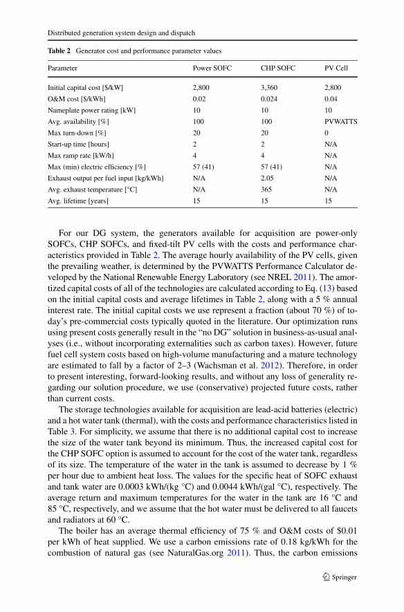
Table 2 Generator cost and performance parameter values

Parameter Power SOFC CHP SOFC PV Cell

Initial capital cost [$/kW] 2,800 3,360 2,800

O&M cost [$/kWh] 0.02 0.024 0.04

Nameplate power rating [kW] 10 10 10

Avg. availability [%] 100 100 PVWATTS

Max turn-down [%] 20 20 0

Start-up time [hours] 2 2 N/A

Max ramp rate [kW/h] 4 4 N/A

Max (min) electric efficiency [%] 57 (41) 57 (41) N/A

Exhaust output per fuel input [kg/kWh] N/A 2.05 N/A

Avg. exhaust temperature [°C] N/A 365 N/A

Avg. lifetime [years] 15 15 15

For our DG system, the generators available for acquisition are power-onlySOFCs, CHP SOFCs, and fixed-tilt PV cells with the costs and performance char-acteristics provided in Table 2. The average hourly availability of the PV cells, giventhe prevailing weather, is determined by the PVWATTS Performance Calculator de-veloped by the National Renewable Energy Laboratory (see NREL 2011). The amor-tized capital costs of all of the technologies are calculated according to Eq. (13) basedon the initial capital costs and average lifetimes in Table 2, along with a 5 % annualinterest rate. The initial capital costs we use represent a fraction (about 70 %) of to-day’s pre-commercial costs typically quoted in the literature. Our optimization runsusing present costs generally result in the “no DG” solution in business-as-usual anal-yses (i.e., without incorporating externalities such as carbon taxes). However, futurefuel cell system costs based on high-volume manufacturing and a mature technologyare estimated to fall by a factor of 2–3 (Wachsman et al. 2012). Therefore, in orderto present interesting, forward-looking results, and without any loss of generality re-garding our solution procedure, we use (conservative) projected future costs, ratherthan current costs.

The storage technologies available for acquisition are lead-acid batteries (electric)and a hot water tank (thermal), with the costs and performance characteristics listed inTable 3. For simplicity, we assume that there is no additional capital cost to increasethe size of the water tank beyond its minimum. Thus, the increased capital cost forthe CHP SOFC option is assumed to account for the cost of the water tank, regardlessof its size. The temperature of the water in the tank is assumed to decrease by 1 %per hour due to ambient heat loss. The values for the specific heat of SOFC exhaustand tank water are 0.0003 kWh/(kg °C) and 0.0044 kWh/(gal °C), respectively. Theaverage return and maximum temperatures for the water in the tank are 16 °C and85 °C, respectively, and we assume that the hot water must be delivered to all faucetsand radiators at 60 °C.

The boiler has an average thermal efficiency of 75 % and O&M costs of $0.01per kWh of heat supplied. We use a carbon emissions rate of 0.18 kg/kWh for thecombustion of natural gas (see NaturalGas.org 2011). Thus, the carbon emissions

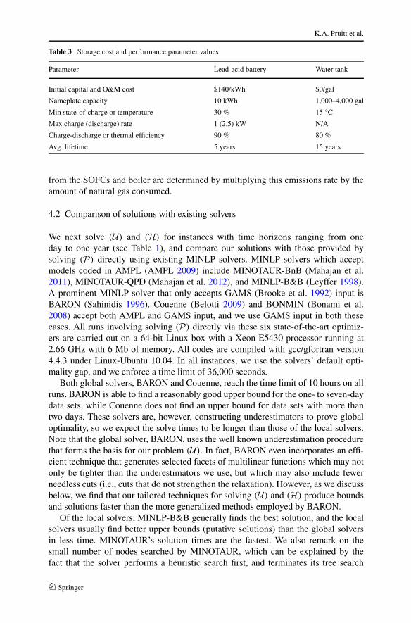
K.A. Pruitt et al.

Table 3 Storage cost and performance parameter values

Parameter Lead-acid battery Water tank

Initial capital and O&M cost $140/kWh $0/gal

Nameplate capacity 10 kWh 1,000–4,000 gal

Min state-of-charge or temperature 30 % 15 °C

Max charge (discharge) rate 1 (2.5) kW N/A

Charge-discharge or thermal efficiency 90 % 80 %

Avg. lifetime 5 years 15 years

from the SOFCs and boiler are determined by multiplying this emissions rate by theamount of natural gas consumed.

4.2 Comparison of solutions with existing solvers

We next solve (U) and (H) for instances with time horizons ranging from oneday to one year (see Table 1), and compare our solutions with those provided bysolving (P) directly using existing MINLP solvers. MINLP solvers which acceptmodels coded in AMPL (AMPL 2009) include MINOTAUR-BnB (Mahajan et al.2011), MINOTAUR-QPD (Mahajan et al. 2012), and MINLP-B&B (Leyffer 1998).A prominent MINLP solver that only accepts GAMS (Brooke et al. 1992) input isBARON (Sahinidis 1996). Couenne (Belotti 2009) and BONMIN (Bonami et al.2008) accept both AMPL and GAMS input, and we use GAMS input in both thesecases. All runs involving solving (P) directly via these six state-of-the-art optimiz-ers are carried out on a 64-bit Linux box with a Xeon E5430 processor running at2.66 GHz with 6 Mb of memory. All codes are compiled with gcc/gfortran version4.4.3 under Linux-Ubuntu 10.04. In all instances, we use the solvers’ default opti-mality gap, and we enforce a time limit of 36,000 seconds.

Both global solvers, BARON and Couenne, reach the time limit of 10 hours on allruns. BARON is able to find a reasonably good upper bound for the one- to seven-daydata sets, while Couenne does not find an upper bound for data sets with more thantwo days. These solvers are, however, constructing underestimators to prove globaloptimality, so we expect the solve times to be longer than those of the local solvers.Note that the global solver, BARON, uses the well known underestimation procedurethat forms the basis for our problem (U). In fact, BARON even incorporates an effi-cient technique that generates selected facets of multilinear functions which may notonly be tighter than the underestimators we use, but which may also include fewerneedless cuts (i.e., cuts that do not strengthen the relaxation). However, as we discussbelow, we find that our tailored techniques for solving (U) and (H) produce boundsand solutions faster than the more generalized methods employed by BARON.

Of the local solvers, MINLP-B&B generally finds the best solution, and the localsolvers usually find better upper bounds (putative solutions) than the global solversin less time. MINOTAUR’s solution times are the fastest. We also remark on thesmall number of nodes searched by MINOTAUR, which can be explained by thefact that the solver performs a heuristic search first, and terminates its tree search

Distributed generation system design and dispatch

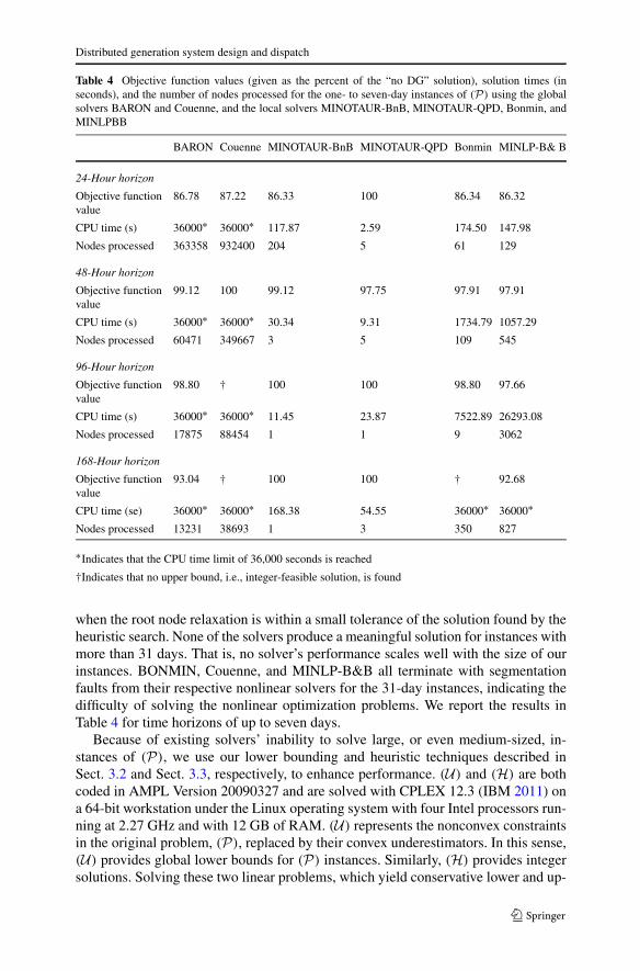
Table 4 Objective function values (given as the percent of the “no DG” solution), solution times (inseconds), and the number of nodes processed for the one- to seven-day instances of (P) using the globalsolvers BARON and Couenne, and the local solvers MINOTAUR-BnB, MINOTAUR-QPD, Bonmin, andMINLPBB

BARON Couenne MINOTAUR-BnB MINOTAUR-QPD Bonmin MINLP-B& B

24-Hour horizon

Objective functionvalue

86.78 87.22 86.33 100 86.34 86.32

CPU time (s) 36000∗ 36000∗ 117.87 2.59 174.50 147.98

Nodes processed 363358 932400 204 5 61 129

48-Hour horizon

Objective functionvalue

99.12 100 99.12 97.75 97.91 97.91

CPU time (s) 36000∗ 36000∗ 30.34 9.31 1734.79 1057.29

Nodes processed 60471 349667 3 5 109 545

96-Hour horizon

Objective functionvalue

98.80 † 100 100 98.80 97.66

CPU time (s) 36000∗ 36000∗ 11.45 23.87 7522.89 26293.08

Nodes processed 17875 88454 1 1 9 3062

168-Hour horizon

Objective functionvalue

93.04 † 100 100 † 92.68

CPU time (se) 36000∗ 36000∗ 168.38 54.55 36000∗ 36000∗Nodes processed 13231 38693 1 3 350 827

∗Indicates that the CPU time limit of 36,000 seconds is reached

†Indicates that no upper bound, i.e., integer-feasible solution, is found

when the root node relaxation is within a small tolerance of the solution found by theheuristic search. None of the solvers produce a meaningful solution for instances withmore than 31 days. That is, no solver’s performance scales well with the size of ourinstances. BONMIN, Couenne, and MINLP-B&B all terminate with segmentationfaults from their respective nonlinear solvers for the 31-day instances, indicating thedifficulty of solving the nonlinear optimization problems. We report the results inTable 4 for time horizons of up to seven days.

Because of existing solvers’ inability to solve large, or even medium-sized, in-stances of (P), we use our lower bounding and heuristic techniques described inSect. 3.2 and Sect. 3.3, respectively, to enhance performance. (U) and (H) are bothcoded in AMPL Version 20090327 and are solved with CPLEX 12.3 (IBM 2011) ona 64-bit workstation under the Linux operating system with four Intel processors run-ning at 2.27 GHz and with 12 GB of RAM. (U) represents the nonconvex constraintsin the original problem, (P), replaced by their convex underestimators. In this sense,(U) provides global lower bounds for (P) instances. Similarly, (H) provides integersolutions. Solving these two linear problems, which yield conservative lower and up-

K.A. Pruitt et al.

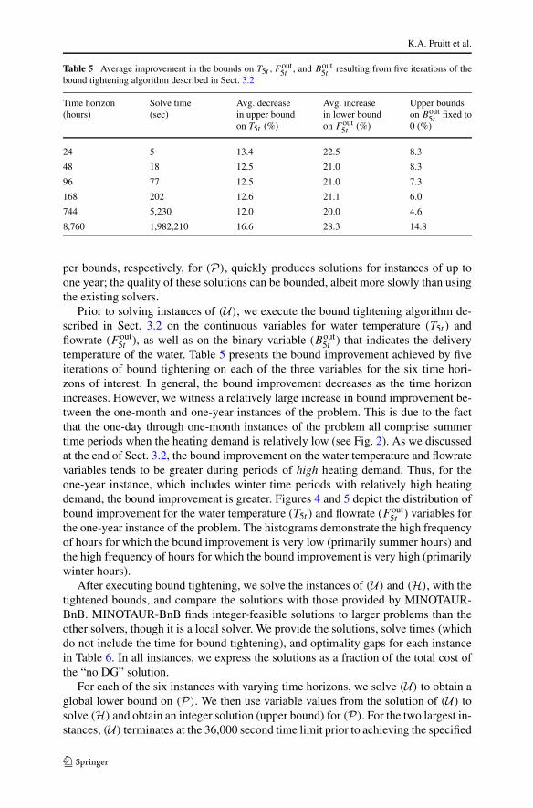
Table 5 Average improvement in the bounds on T5t , Fout5t

, and Bout5t

resulting from five iterations of thebound tightening algorithm described in Sect. 3.2

Time horizon(hours)

Solve time(sec)

Avg. decreasein upper boundon T5t (%)

Avg. increasein lower boundon F out

5t(%)

Upper boundson Bout

5tfixed to

0 (%)

24 5 13.4 22.5 8.3

48 18 12.5 21.0 8.3

96 77 12.5 21.0 7.3

168 202 12.6 21.1 6.0

744 5,230 12.0 20.0 4.6

8,760 1,982,210 16.6 28.3 14.8

per bounds, respectively, for (P), quickly produces solutions for instances of up toone year; the quality of these solutions can be bounded, albeit more slowly than usingthe existing solvers.

Prior to solving instances of (U), we execute the bound tightening algorithm de-scribed in Sect. 3.2 on the continuous variables for water temperature (T5t ) andflowrate (F out

5t ), as well as on the binary variable (Bout5t ) that indicates the delivery

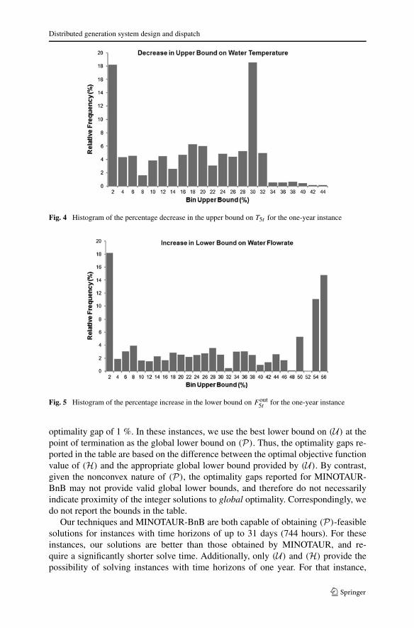
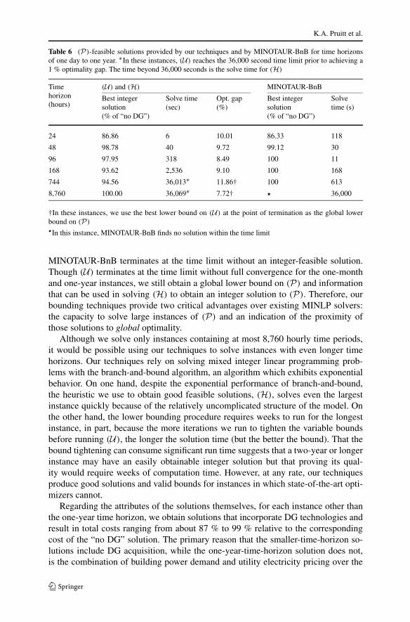
temperature of the water. Table 5 presents the bound improvement achieved by fiveiterations of bound tightening on each of the three variables for the six time hori-zons of interest. In general, the bound improvement decreases as the time horizonincreases. However, we witness a relatively large increase in bound improvement be-tween the one-month and one-year instances of the problem. This is due to the factthat the one-day through one-month instances of the problem all comprise summertime periods when the heating demand is relatively low (see Fig. 2). As we discussedat the end of Sect. 3.2, the bound improvement on the water temperature and flowratevariables tends to be greater during periods of high heating demand. Thus, for theone-year instance, which includes winter time periods with relatively high heatingdemand, the bound improvement is greater. Figures 4 and 5 depict the distribution ofbound improvement for the water temperature (T5t ) and flowrate (F out

5t ) variables forthe one-year instance of the problem. The histograms demonstrate the high frequencyof hours for which the bound improvement is very low (primarily summer hours) andthe high frequency of hours for which the bound improvement is very high (primarilywinter hours).

After executing bound tightening, we solve the instances of (U) and (H), with thetightened bounds, and compare the solutions with those provided by MINOTAUR-BnB. MINOTAUR-BnB finds integer-feasible solutions to larger problems than theother solvers, though it is a local solver. We provide the solutions, solve times (whichdo not include the time for bound tightening), and optimality gaps for each instancein Table 6. In all instances, we express the solutions as a fraction of the total cost ofthe “no DG” solution.

For each of the six instances with varying time horizons, we solve (U) to obtain aglobal lower bound on (P). We then use variable values from the solution of (U) tosolve (H) and obtain an integer solution (upper bound) for (P). For the two largest in-stances, (U) terminates at the 36,000 second time limit prior to achieving the specified

Distributed generation system design and dispatch

Fig. 4 Histogram of the percentage decrease in the upper bound on T5t for the one-year instance

Fig. 5 Histogram of the percentage increase in the lower bound on F out5t

for the one-year instance

optimality gap of 1 %. In these instances, we use the best lower bound on (U) at thepoint of termination as the global lower bound on (P). Thus, the optimality gaps re-ported in the table are based on the difference between the optimal objective functionvalue of (H) and the appropriate global lower bound provided by (U). By contrast,given the nonconvex nature of (P), the optimality gaps reported for MINOTAUR-BnB may not provide valid global lower bounds, and therefore do not necessarilyindicate proximity of the integer solutions to global optimality. Correspondingly, wedo not report the bounds in the table.

Our techniques and MINOTAUR-BnB are both capable of obtaining (P)-feasiblesolutions for instances with time horizons of up to 31 days (744 hours). For theseinstances, our solutions are better than those obtained by MINOTAUR, and re-quire a significantly shorter solve time. Additionally, only (U) and (H) provide thepossibility of solving instances with time horizons of one year. For that instance,

K.A. Pruitt et al.

Table 6 (P)-feasible solutions provided by our techniques and by MINOTAUR-BnB for time horizonsof one day to one year. ∗In these instances, (U) reaches the 36,000 second time limit prior to achieving a1 % optimality gap. The time beyond 36,000 seconds is the solve time for (H)

Timehorizon(hours)

(U) and (H) MINOTAUR-BnB

Best integersolution(% of “no DG”)

Solve time(sec)

Opt. gap(%)

Best integersolution(% of “no DG”)

Solvetime (s)

24 86.86 6 10.01 86.33 118

48 98.78 40 9.72 99.12 30

96 97.95 318 8.49 100 11

168 93.62 2,536 9.10 100 168

744 94.56 36,013∗ 11.86† 100 613

8,760 100.00 36,069∗ 7.72† � 36,000

†In these instances, we use the best lower bound on (U) at the point of termination as the global lowerbound on (P)

�In this instance, MINOTAUR-BnB finds no solution within the time limit

MINOTAUR-BnB terminates at the time limit without an integer-feasible solution.Though (U) terminates at the time limit without full convergence for the one-monthand one-year instances, we still obtain a global lower bound on (P) and informationthat can be used in solving (H) to obtain an integer solution to (P). Therefore, ourbounding techniques provide two critical advantages over existing MINLP solvers:the capacity to solve large instances of (P) and an indication of the proximity ofthose solutions to global optimality.

Although we solve only instances containing at most 8,760 hourly time periods,it would be possible using our techniques to solve instances with even longer timehorizons. Our techniques rely on solving mixed integer linear programming prob-lems with the branch-and-bound algorithm, an algorithm which exhibits exponentialbehavior. On one hand, despite the exponential performance of branch-and-bound,the heuristic we use to obtain good feasible solutions, (H), solves even the largestinstance quickly because of the relatively uncomplicated structure of the model. Onthe other hand, the lower bounding procedure requires weeks to run for the longestinstance, in part, because the more iterations we run to tighten the variable boundsbefore running (U), the longer the solution time (but the better the bound). That thebound tightening can consume significant run time suggests that a two-year or longerinstance may have an easily obtainable integer solution but that proving its qual-ity would require weeks of computation time. However, at any rate, our techniquesproduce good solutions and valid bounds for instances in which state-of-the-art opti-mizers cannot.

Regarding the attributes of the solutions themselves, for each instance other thanthe one-year time horizon, we obtain solutions that incorporate DG technologies andresult in total costs ranging from about 87 % to 99 % relative to the correspondingcost of the “no DG” solution. The primary reason that the smaller-time-horizon so-lutions include DG acquisition, while the one-year-time-horizon solution does not,is the combination of building power demand and utility electricity pricing over the

Distributed generation system design and dispatch

time horizon of interest. The one-month and shorter time horizons comprise onlysummer time periods. Based on the demand and pricing data depicted in Figs. 2 and3, respectively, the building power demand and utility electricity pricing are both rel-atively high in the summer. Thus, the savings provided by operating a DG systemto meet the building’s power demands, versus purchasing all of the electricity fromthe utility, are relatively high during the summer. As a result, DG acquisition is moreeconomically attractive when only summer time periods are considered. By contrast,when we consider the entire year, which includes winter time periods with relativelylower power demand and electricity pricing, the savings provided by DG are rela-tively lower and the technologies are less economically attractive.

Another reason that the lowest-cost solution we obtain for the one-year instance isno better than the “no DG” solution is that the capital costs are 70 % of today’s pre-commercial costs, a percentage that is still relatively high compared with purchasingpower from the grid at costs current at the time of this writing. Were we to reduce thispercentage, we would see investments in the DG technologies. Indeed, these capitalcosts are likely to decrease over time, making future capital installation costs 30 %of today’s costs realistic. All of our computational procedures (i.e., the heuristic andthe lower bounding techniques) are generalizable so, indeed, it would be possible tocreate other scenarios with lower capital costs, solving them using our procedures.

5 Conclusions

In this paper, we present an optimization model which determines the configuration,capacity, and operational schedule of a DG system capable of meeting the powerand heat demands of a commercial building at the globally minimum total cost. Themodel includes aspects of the system operation that are not considered in other re-search. In particular, we model the operational status, ramping capacity, and variableelectric efficiency of power generation technologies. Additionally, we model thermalstorage as a function of the temperature at which hot water is stored. These modelinginnovations allow us to capture detailed system performance characteristics and toobtain realistic solutions. However, those same innovations require additional integervariables in every time period and nonlinearities that dictate our system be modeledas a large, nonconvex MINLP.

The algorithms capable of solving large, nonconvex MINLPs to global optimal-ity are limited. In order to execute a nonlinear branch-and-bound algorithm that iscapable of solving such problems to global optimality, we require methods for deter-mining global lower and upper bounds on the optimal objective function value at eachnode of the branch-and-bound tree. Yet, solving the continuous relaxation of a non-convex MINLP may not lead to a global lower bound and currently available solversare not capable of solving large instances of nonconvex MINLPs to obtain a globalupper bound. As a result, we formulate a convex underestimation of our MINLP toobtain a global lower bound and develop a linearization heuristic to obtain a globalupper bound.

We demonstrate our bounding techniques for model instances ranging in size fromone day to one year using a large hotel located in Los Angeles, CA as a case study.

K.A. Pruitt et al.

We then compare our solutions with those provided by existing solvers. Few exist-ing solvers are capable of obtaining solutions for instances of our MINLP with timehorizons of longer than one week. Those that can solve these instances offer little tono improvement over the solutions provided by our techniques and require a longerrun time. Furthermore, our techniques present the possibility to solve larger instancesof the problem that exceed the capacity of existing solvers. The ability to solve theselarger instances is critical to the real-world application of the model to inform long-term capital investment decisions. Specifically, our ability to capture an entire year’sworth of data to produce a solution provides us with a better representation of thecost-minimizing operation of a system and the corresponding optimal design. Werewe to capture only a representative day for each season in our scenario, we wouldbe omitting the day-to-day fluctuations that occur, and we would be assuming thatwe could employ a method (in terms of the variables for which our model determinesvalues) for addressing these fluctuations. Such a method would rely upon the assump-tion that there is only a finite number of seasons within a year, each of which could becharacterized by a representative day. While this may be a reasonable approximation,it is certainly not realistic; there are transitions between days, or seasons, character-ized by, for example, a slow increase in the heating demand. Such a trend could notbe adequately captured nor optimally accounted for in the design and operation of aDG system without the explicit incorporation of the hours, or days, that exhibit thetrend.

The solutions obtained from our model provide valuable insights into the acquisi-tion and operation of commercial sector DG systems. Additionally, sensitivity analy-ses have the potential to influence future energy policy measures. The parameters forutility pricing, carbon taxation, building demand, DG capital and operational costs,and DG technological performance can all be analyzed within the context of ourmodel to determine the conditions for which DG is most economically and environ-mentally viable. Further research could also include uncertainty in building demand,system output, and utility pricing to test the robustness of the system design solu-tions. With such computational tools providing both critical information and quan-titative assessments of the energetic and economic benefits of DG-based solutions,CHP and other distributed energy resources might finally achieve substantial marketpenetration.

Acknowledgements The authors would like to thank the National Science Foundation for partial sup-port of this research effort under award #CNS-0931748. We are also grateful to Andrew Schmidt, Depart-ment of Mechanical Engineering, Colorado School of Mines, for providing the building load data fromEnergyPlus.

References

Adjiman C, Floudas C (2008) αBB algorithm. In: Encyclopedia of Optimization, vol 1. Kluwer Academic,Norwell, pp 61–73

AMPL (2009) AMPL version 10.6.16. AMPL optimization LLCBao X, Sahinidis N, Tawarmalani M (2009) Multiterm polyhedral relaxations for nonconvex,

quadratically-constrained quadratic programs. Optim Methods Softw 24(4–5):485–504Belotti P (2009) COUENNE: a user’s manual. Tech rep, Lehigh University. https://projects.coin-or.org/

Couenne/browser/trunk/Couenne/doc/couenne-user-manual.pdf?format=raw

Distributed generation system design and dispatch

Bonami P, Biegler L, Conn A, Cornuéjols G, Grossmann I, Laird C, Lee J, Lodi A, Margot F, Sawaya N,Wächter A (2008) An algorithmic framework for convex mixed integer nonlinear programs. DiscreteOptim 5(2):186–204

Brooke A, Kendrick D, Meeraus A (1992) GAMS—a user’s guide (release 2.25). Boyd & Fraser, DanversBurer M, Tanaka K, Favrat D, Yamada K (2003) Multi-criteria optimization of a district cogeneration

plant integrating a solid oxide fuel cell-gas turbine combined cycle, heat pumps and chillers. Energy28(6):497–518

DOE (2010) Getting started with EnergyPlus: basic concepts manual-information you need about runningEnergyPlus

EIA (2011a) Annual energy outlook (AEO2011). Early release overviewEIA (2011b) Summary statistics for electric power in the US, 1998–2009Georgilakis P (2006) State-of-the-art of decision support systems for the choice of renewable energy

sources for energy supply in isolated regions. Int J Distrib Energy Resour 2(2):129–150Greene N, Hammerschlag R (2000) Small and clean is beautiful: exploring the emissions of distributed

generation and pollution prevention policies. Electr J 13(5):50–60Gumerman E, Bharvirkar R, LaCommare K, Marnay C (2003) Evaluation framework and tools for dis-

tributed energy resources. Tech rep LBNL-52079, Lawrence Berkeley National LaboratoryIBM (2011) IBM ILOG AMPL version 12.3 user’s guide: standard (command-line) version including

CPLEX directivesKaffine D, McBee B, Lieskovsky J (2011) Empirical estimates of emissions avoided from wind power

generation. USAEE Dialogue 19(1)Leyffer S (1998) User manual for MINLP-BB. University of DundeeMahajan A, Leyffer S, Kirches C (2012) Solving mixed-integer nonlinear programs by QP-diving. Preprint

ANL/MCS-2071-0312, Argonne National Laboratory, Mathematics and Computer Science DivisionMahajan A, Leyffer S, Linderoth J, Luedtke J, Munson T (2011) MINOTAUR: a toolkit for solving mixed-

integer nonlinear optimization. Wiki-page http://wiki.mcs.anl.gov/minotaurMcCormick G (1976) Computability of global solutions to factorable nonconvex programs. Part 1. Convex

underestimating problems. Math Program 10:147–175NaturalGas.org (2011) Natural gas and the environmentNicholson W, Snyder C (2008) Microeconomic theory: basic principles and extensions, 10th edn. South-

WesternNREL (2011) A performance calculator for grid-connected PV systems (PVWATTSv.1)Sahinidis N (1996) BARON: a general purpose global optimization software package. J Glob Optim

8(2):201–205SCE (2010) Schedule TOU-GS-3SCGC (2010) Schedule G-10Siddiqui A, Marnay C, Bailey O, LaCommare K (2005a) Optimal selection of on-site generation with

combined heat and power applications. Int J Distrib Energy Resour 1(1):33–62Siddiqui A, Marnay C, Firestone R, Zhou N (2005) Distributed generation with heat recovery and storage.

Tech rep LBNL-58630, Lawrence Berkeley National LaboratoryTawarmalani M, Sahinidis N (2003) A polyhedral branch-and-cut approach to global optimization. Math

Program 103(2):225–249Wachsman E, Marlowe A, Lee K (2012) Role of solid oxide fuel cells in a balanced energy strategy. Energ

Environ Sci 5(2):5498–5509Weber C, Marechal F, Favrat D, Kraines S (2006) Optimization of an SOFC-based decentralized poly-

generation system for providing energy services in an office-building in Tokyo. Appl Therm Eng26(13):1409–1419