a minimal-variable symplectic integrator on spheres · a minimal-variable symplectic integrator on...
TRANSCRIPT

A minimal-variable symplectic integrator onspheres
Robert McLachlan∗1, Klas Modin†2, and Olivier Verdier‡3
1 Institute of Fundamental Sciences, Massey University, New Zealand2 Mathematical Sciences, Chalmers University of Technology, Sweden
3 Department of Computing, Mathematics and Physics, Western Norway University of AppliedSciences, Bergen, Norway
2017-05-19
We construct a symplectic, globally defined, minimal-variable, equivariantintegrator on products of 2-spheres. Examples of corresponding Hamiltoniansystems, called spin systems, include the reduced free rigid body, the motionof point vortices on a sphere, and the classical Heisenberg spin chain, aspatial discretisation of the Landau–Lifshitz equation. The existence of suchan integrator is remarkable, as the sphere is neither a vector space, nor acotangent bundle, has no global coordinate chart, and its symplectic form isnot even exact. Moreover, the formulation of the integrator is very simple,and resembles the geodesic midpoint method, although the latter is notsymplectic.
1. Introduction
The 2–sphere, denoted S2, is a fundamental symplectic manifold that occurs as the phasespace, or part of the phase space, of many Hamiltonian systems in mathematical physics.A globally defined symplectic integrator on S2 needs a minimum of three variables, sincethe lowest-dimensional vector space in which S2 can be embedded is R3. To constructsuch a minimal-variable, symplectic integrator is, however, surprisingly difficult, and haslong been an open problem. Here we solve that problem. We equip the direct product of
∗[email protected]†[email protected]‡[email protected]
1
arX
iv:1
402.
3334
v5 [
mat
h-ph
] 1
8 M
ay 2
017

n 2-spheres, (S2)n, with the symplectic form ω given by the weighted sum of the areaforms
ω =n∑i=1
κidAi, κi > 0, (1)
where dAi is the standard area form on the i:th sphere.Throughout the paper, we represent S2 by the space of unitary vectors in R3. General
Hamiltonian systems on (S2)n with respect to the symplectic form (1) take the form
wi = wi ×1
κi
∂H
∂wi, wi ∈ S2, i = 1, . . . , n, H ∈ C∞((S2)n). (2)
We provide a global, second order symplectic integrator for such systems, which we callthe spherical midpoint method. The method is remarkably simple: for a Hamiltonianfunction H ∈ C∞((S2)n), it is the mapping(
S2)n 3 (w1, . . . ,wn) 7→
(W 1, . . . ,W n
)∈(S2)n,
defined by
W i −wi
h=wi +W i
|wi +W i|× 1
κi
∂H
∂wi
(w1 +W 1
|w1 +W 1|, . . . ,
wn +W n
|wn +W n|
),
where h > 0 is the step size. In addition to be symplectic, this method is equivariant,meaning it respects the intrinsic symmetries of the 2–sphere. Put differently, it respectsthe homogeneous space structure S2 ' SO(3)/SO(2), a property analogous to the affineequivariance of B-series methods [24]. Note also, as we observe in Remark 2.2, that ourmethod is not the geodesic midpoint method applied to (2).
Equations of the form (2) are called classical spin systems [14]. The simplest exampleis the reduced free rigid body
w = w × I−1w, w ∈ S2.
Other examples include the motion of massless particles in a divergence-free vector fieldon the sphere (for example, test particles in a global weather simulation), the motion of npoint vortices in a ideal incompressible fluid on the sphere, and the set of Lie–Poissonsystems on so(3)∗. Spin systems with large n are obtained by spatial discretisationsof Hamiltonian PDEs on S2. An example is the classical Heisenberg spin chain ofmicromagnetics,
wi = wi × (wi+1 − 2wi +wi−1), w0 = wn, wi ∈ S2,
which is a spatial discretisation of the Landau–Lifshitz PDE
w = w ×w′′, w ∈ C∞(S1, S2).
Apart from its abundance in physics, there are a number of reasons for focusing on thephase space (S2)n. It is the first example of a symplectic manifold that
2

• is not a vector space,
• is not a cotangent bundle,
• does not have a global coordinate chart or a cover with one, and
• is not exact (that is, the symplectic form is not exact).
Furthermore, next to cotangent bundles, the two main types of symplectic manifolds arecoadjoint orbits of Lie–Poisson manifolds and Kahler manifolds; (S2)n is the simplestexample of both of these.
Lie group integrators for general systems on (S2)n are developed in [18]. These are,however, not symplectic. Symplectic integrators for some classical spin systems aregiven in [35, 20]. These are, however, based on splitting, and therefore not applicable forgeneral Hamiltonians.
To find symplectic integrators on (S2)n for general Hamiltonians is particularly chal-lenging because symplectic integrators for general Hamiltonians are closely related to theclassical canonical generating functions defined on symplectic vector spaces (or in localcanonical coordinates). Generating functions are a tool of vital importance in mechanics,used for perturbation theory, construction of orbits and of normal forms, in bifurcationtheory, and elsewhere. They have retained their importance in the era of symplecticgeometry and topology, being used to construct Lagrangian submanifolds and to countperiodic orbits [37, 36]. Although there are different types of generating function, all ofthem are restricted to cotangent bundle phase spaces.
In our case, the four ‘classical’ generating functions, that treat the position andmomentum differently, do not seem to be relevant given the symmetry of S2. Instead,our novel method (or generating function) is more related to the Poincare generatingfunction [32, vol. III, §319]
J(W −w) = ∇G(W +w
2
), J =
(0 I−I 0
),
which is equivariant with respect to the full affine group and which corresponds to theclassical midpoint method when interpreted as a symplectic integrator. The classicalmidpoint method on vector spaces is known to conserve quadratic invariants [6], andhence automatically induces a map on S2 when applied to spin systems. However, it haslong been known not to be symplectic [2].
We now list the already known techniques to construct symplectic integrators forgeneral Hamiltonian systems on a symplectic manifold M that is not a vector space:
1. If M = T ∗Q is the cotangent bundle of a submanifold Q ⊂ Rn determined by levelsets of m functions c1, . . . , cm, then the family of RATTLE methods can be used [10].More generally, if M is a transverse submanifold of R2n defined by coisotropicconstraints, then geometric RATTLE methods can be used [27].
2. If M ⊂ g∗ is a coadjoint orbit (symplectic leaf) of the dual of a Lie algebra gcorresponding to a Lie group G, RATTLE methods can again be used: first extend
3
the symplectic system on M to a Poisson system on g∗, then “unreduce” to asymplectic system on T ∗G, then embed G in a vector space and use strategy 1above [8, §VII.5]. One can also use Lie group integrators for the unreduced systemon T ∗G [4, 22]. The discrete Lagrangian method, pioneered in this context byMoser and Veselov [29], yields equivalent classes of methods. The approach is verygeneral, containing a number of choices, especially those of the embedding and thediscrete Lagrangian. For certain choices, in some cases, such as the free rigid body,the resulting discrete equations are completely integrable; this observation has beenextensively developed [7].
3. If M ⊂ g∗ is a coadjoint orbit and g∗ has a symplectic realisation on R2n obtainedthrough a momentum map associated with a Hamiltonian action of G on R2n,then symplectic Runge–Kutta methods for collective Hamiltonian systems (cf. [21])sometimes descend to symplectic methods on M (so far, the cases sl(2)∗, su(n)∗,so(n)∗, and sp(n)∗ have been worked out). This approach leads to collectivesymplectic integrators [25].
Let us review these approaches for the case M = S2.The first approach is not applicable, since S2 is not a cotangent bundle.The second approach is possible, since S2 is a coadjoint orbit of su(2)∗ ' R3. SU(2)
can be embedded as a 3–sphere in R4 using unit quaternions, which leads to methodsthat use 10 variables, in the case of RATTLE (8 dynamical variables plus 2 Lagrangemultipliers), and 8 variables, in the case of Lie group integrators. Both of these methodsare complicated; the first due to constraints and the second due to the exponential mapand the need to solve nonlinear equations in auxiliary variables.
The third approach is investigated in [26]. It relies on a quadratic momentum mapπ : T ∗R2 → su(2)∗ and integration of the system corresponding to the collective Hamil-tonian H ◦ π using a symplectic Runge–Kutta method. This yields relatively simpleintegrators using 4 variables. They rely on an auxiliary structure (the suspension toT ∗R2 and the Poisson property of π) and requires solving nonlinear equations in auxiliaryvariables; although simple, they do not fully respect the simplicity of S2.
Our spherical midpoint method, fully described in § 2, is simpler than all of the knownapproaches above; it is as simple as the classical midpoint method on vector spaces. Wewould like to emphasise, however, that symplecticity of our method is by no means relatedto the symplecticity of the classical midpoint method. The existence of the sphericalmidpoint method is thus unexpected, and its symplecticity is surprisingly difficult toprove.
In § 3 we provide a series of detailed numerical examples for various spin systems.Interestingly, the error constants for the spherical midpoint method appears to besignificantly smaller than for the RATTLE method.
Finally, while the present study is phrased in the language of numerical integration,we wish to remind the reader of the strong relation to discrete time mechanics, a fieldstudied for many reasons:
(i) It has an immediate impact in computational physics, where symplectic integrators
4

are in widespread use and in many situations are overwhelmingly superior tostandard numerical integration [28].
(ii) As a generalisation of continuous mechanics, discrete geometric mechanics is inprinciple more involved: the nature of symmetries, integrals, and other geometricconcepts is important to understand both in its own right and for its impact onnumerical simulations [8].
(iii) Discretisation leads to interesting physics models, for example the extensively-studied Chirikov standard map [5].
(iv) Discrete models can also be directly relevant to intrinsically discrete situations,such as waves in crystal lattices. Here, the appearance of new phenomena, notpersisting at small or vanishing lattice spacing, is well known [11].
(v) The field of discrete integrability is undergoing rapid evolution, with many newexamples, approaches, and connections to other branches of mathematics, e.g.,special functions and representation theory [13].
(vi) A strand of research in physics, pioneered notably by Lee [16], develops the ideathat time is fundamentally discrete, and it is the continuum models that are theapproximation.
(vii) Discrete models can contain “more information and more symmetry than the corre-sponding differential equations” [17]; this also occurs in discrete integrability [13].
2. Main results
We present our two methods, the spherical midpoint method, and the extended sphericalmidpoint method, and state their properties.
We use the following notation. X(M) denotes the space of smooth vector fields on amanifold M . If M is a Poisson manifold, and H ∈ C∞(M) is a smooth function on M ,then the corresponding Hamiltonian vector field is denoted XH . The Euclidean lengthof a vector w ∈ Rd is denoted |w|. If w ∈ R3n ' (R3)n, then wi denotes the i:thcomponent in R3.
2.1. Spherical Midpoint Method: Symplectic integrator on spheres
Our paper is devoted to the following novel method.
Definition 2.1. The spherical midpoint method for ξ ∈ X((S2)n
)is the numerical
integratorΦ(hξ) : (S2)n → (S2)n, (3)
obtained as a mapping w →W , with w, W in (S2)n, by
W −w = hξ( (w +W )1
|(w +W )1|, . . . ,
(w +W )n|(w +W )n|
). (4)
5

Remark 2.2. Note that, even for n = 1, the spherical midpoint method is not thegeodesic midpoint method on the sphere. Let m(w,W ) denote the geodesic midpoint ofw and W , and let d(w,W ) denote the geodesic (great-circle) distance between w and W .The geodesic midpoint method is defined by the conditions that ξ(m(w,W )) is tangentto the geodesic between w and W , and that d(w,W ) = |hξ(m(w,W ))|. The sphericalmidpoint method (4) fulfills the first of these conditions, but not the second: ξ(m(w,W ))is tangent to the geodesic between w and W , but 2 sin
(d(w,W )/2
)= |hξ(m(w,W ))|.
Recall now the definition of the classical midpoint method:
Definition 2.3. The classical midpoint method for discrete time approximation ofthe ordinary differential equation w = X(w), X ∈ X(Rd), is the mapping w 7→ Wdefined by
W −w = hX(W +w
2
), (5)
where h > 0 is the time-step length.
Define a projection map ρ by
ρ(w) =( w1
|w1|, . . . ,
wn
|wn|
). (6)
It is clear that the spherical midpoint method (4) is obtained by defining the vectorfield given by
X(w) := ξ(ρ(w)). (7)
and then use the classical midpoint method (5) with the vector field X. Notice that X isnot defined whenever wi = 0 for some i. In practice this is never a problem, since we areinterested in vector fields preserving the spheres.
This indeed gives an integrator on (S2)n, since the classical midpoint method preservesquadratic invariants, and the vector field (7) is tangent to the spheres (which are thelevel sets of quadratic functions on R3n).
We now give the main result of the paper.
Theorem 2.4. The spherical midpoint method (3) fulfils the following properties:
(i) it is symplectic with respect to ω if ξ is Hamiltonian with respect to ω;
(ii) it is second order accurate;
(iii) it is equivariant with respect to(SO(3)
)nacting on (S2)n, i.e.,
ψg−1 ◦ Φ(hξ) ◦ ψg = Φ(hψ∗gξ), ∀ g = (g1, . . . , gn) ∈(SO(3)
)n,
where ψg is the action map;
(iv) it preserves arbitrary linear symmetries, arbitrary linear integrals, and single-spinhomogeneous quadratic integrals w>i Awi;
6

(v) it is self-adjoint and preserves arbitrary linear time-reversing symmetries;
(vi) it is linearly stable: for the linear ODE w = λw × a, the method yields a rotationabout the unit vector a by an angle cos−1(1 − 1
2(λh)2) and hence is stable for0 ≤ λh < 2.
Proof. We use on several occasions the observation that the spherical midpoint methodcan be reformulated as the classical midpoint method applied to the vector field (7),using the projection map ρ defined in (6).
(i) The proof is postponed to § 2.3.
(ii) The midpoint method is of order 2, and a solution to w = X(w) with X givenby (7) is also a solution to w = ξ(w).
(iii) The map ρ is equivariant with respect to(SO(3)
)n,(SO(3)
)nis a subgroup of the
affine group on R3n and the classical midpoint method is affine equivariant.
(iv), (v) Direct calculations show that X has the same properties in the given cases as theoriginal vector field ξ, and the classical midpoint method is known to preserve theseproperties.
(vi) The projection ρ renders the equations for the method nonlinear, even for thislinear test equation; it is clear that the solution is a rotation about a by someangle; this yields a nonlinear equation for the angle with the given solution.
Remark 2.5. Note that the unconditional linear stability of the classical midpointmethod is lost for the spherical midpoint method; the method’s response to the harmonicoscillator is identical to that of the leapfrog (Stormer–Verlet) method.
Remark 2.6. The spherical midpoint method is second order accurate. Since it is alsosymmetric, one can use symmetric composition techniques, as described in [8, §V.3.2], toobtain higher order symplectic integrators on (S2)n.
2.2. Spherical Midpoint Method: Lie–Poisson integrator
R3n is a Lie–Poisson manifold with Poisson bracket
{F,G}(w) =n∑k=1
(∂F (w)
∂wk× ∂G(w)
∂wk
)·wk. (8)
This is the canonical Lie–Poisson structure of (so(3)∗)n, or (su(2)∗)n, obtained byidentifying so(3)∗ ' R3, or su(2)∗ ' R3. For details, see [23, § 10.7] or [26].
The Hamiltonian vector field associated with a Hamiltonian function H : R3n → R isgiven by
XH(w) =n∑k=1
wk ×∂H(w)
∂wk.
7

λ
Figure 1: Structure of the Lie–Poisson manifold (R3, {·, ·}). Lie–Poisson manifolds arefoliated by symplectic submanifolds (symplectic leaves) given by the coadjointorbits. For R3 equipped with the Poisson bracket (8), the coadjoint orbitsare given by the submanifolds S2
λ ⊂ R3. Thus, to construct a Lie–Poissonintegrator on R3n is equivalent to constructing symplectic integrators for thesymplectic direct product manifolds S2
λ1× · · · × S2
λn.
Its flow, exp(XH), preserves the Lie–Poisson structure, i.e.,
{F ◦ exp(XH), G ◦ exp(XH)} = {F,G} ◦ exp(XH), ∀F,G ∈ C∞(R3n).
The flow exp(XH) also preserves the coadjoint orbits [23, § 14], given by
S2λ1 × · · · × S
2λn ⊂ R3n, λ1, . . . , λn ≥ 0,
where S2λ denotes the 2–sphere in R3 of radius λ. A Lie–Poisson integrator for XH is an
integrator that, like the exact flow, preserves the Lie–Poisson structure and the coadjointorbits. For an illustration of the coadjoint orbits, see Figure 1.
Definition 2.7. The extended spherical midpoint method for X ∈ X(R3n) is thenumerical integrator defined by
W −w = hX
(√|w1||W 1|(w1 +W 1)
|w1 +W 1|, . . . ,
√|wn||W n|(wn +W n)
|wn +W n|
). (9)
We define the expression
√|wi||W i|(wi+W i)
|wi+W i| to be zero whenever the denominator is
zero. The equation (9) is thereby defined on all of R3n.We have the following result, analogous to Theorem 2.4.
Theorem 2.8. The extended spherical midpoint method (9) fulfils the following properties:
(i) it is a Lie–Poisson integrator for Hamiltonian vector fields XH ∈ X(R3n);
(ii) it is second order accurate;
(iii) it is equivariant with respect to(SO(3)
)nacting diagonally on (R3)n ' R3d (the
diagonal action is defined by (g1, . . . , gn) · (w1, . . . ,wn) = (g1w1, . . . , gnwn)).
8

(iv) it preserves arbitrary linear symmetries, arbitrary linear integrals, and single-spinhomogeneous quadratic integrals w>i Awi, where A ∈ R3×3;
(v) it is self-adjoint and preserves arbitrary linear time-reversing symmetries;
Proof. For convenience, we define Γ: R3n ×R3n → R3n by
Γ(w,W
):=
(√|w1||W 1|(w1 +W 1)
|w1 +W 1|, . . . ,
√|wn||W n|(wn +W n)
|wn +W n|
).
(i) The proof is postponed to § 2.3.
(ii) First notice that
Γ(w,W ) =w +W
2+O(|W −w|) (10)
Using (10) in (9), and using that X is smooth, we obtain
W −w = hX(w +W
2
)+ hO(|W −w|).
We use (9) again to obtain
W −w = hX(w +W
2
)+ h2O
(∣∣X(Γ(w,W ))∣∣).
Since Γ(w,W ) is bounded for fixed w, we get W = W + O(h2), where W isthe solution obtained by the classical midpoint method (5) on R3n. The methoddefined by (9) is therefore at least first order accurate. Second order accuracyfollows since the method is symmetric.
(iii) Γ is equivariant with respect to (SO(3))n, so we obtain SO(3) equivariance of themethod.
(iv), (v) Same proof as in Theorem 2.4.
2.3. Proof of symplecticity
We need some preliminary definitions and results before the main proof.
Definition 2.9. The ray through a point w ∈ R3n is the subset
{(λ1w1, . . . , λnwn);λ ∈ Rn+}.
The set of all rays is in one-to-one relation with (S2)n. Note that the vector field Xdefined by (7) is constant on rays. The following result, essential throughout theremainder of the paper, shows that the property of being constant on rays is passed onfrom Hamiltonian functions to Hamiltonian vector fields.
9

Lemma 2.10. If a Hamiltonian function H ∈ C∞((R3\{0})n) is constant on rays, thenso is its Hamiltonian vector field XH .
Proof. It is enough to consider n = 1, as the general case proceeds the same way. H isconstant on rays, so for λ > 0, we have
H(λw) = H(w).
Differentiating with respect to w yields
λ∇H(λw) = ∇H(w)
The Hamiltonian vector field at λw is
XH(λw) = λw ×∇H(λw)
= w ×∇H(w)
= XH(w),
which proves the result.
Recall that if X is any vector field on Rn, then tangent vectors u(t) to integral curvesw(t) of X obey the variational equation u = DX(w(t))u, where u ∈ Tw(T )R
n. Thefollowing lemma establishes the equivalent result for transport of 1-forms. We representthe 1-form
∑ni=1 σidwi ∈ T ∗wRn by the column vector σ.
Lemma 2.11. Let ϕ(t) the flow of the vector field X on Rn and w(t) an integral curve.Let σ(t) be a curve of 1-forms transported by the flow, i.e., such that ϕ(t)∗σ(t) = σ(0).Then σ = −DX(w(t))>σ.
Proof. For all u ∈ Tw(0)Rn we have 〈ϕ(t)∗σ(t),u〉 = 〈σ(t), Dϕ(t)u〉, so that σ(0)>u =
σ(t)>Dϕ(t)u or σ(0) = Dϕ(t)>σ(t). Differentiating with respect to t at t = 0 and usingDϕ(0) = I, ϕ(0) = X gives the result.
Any Poisson bracket on a manifold M is associated with a Poisson bivector K, a sectionof∧2(TM), such that {F,G}(w) = K(w)
(dF (w),dG(w)
). The flow of a Hamiltonian
vector field preserves the Poisson structure (see, e.g., [23], Prop. 10.3.1), which in termsof K is the statement that d
dtK(w(t)(σ(t), λ(t))=0. In the Lie–Poisson case, K is linearin w, so using the product rule together with linearity in each of the 3 arguments gives
K(w)(σ, λ) +K(w)(σ, λ) +K(w)(σ, λ) = 0 (11)
where w = XH(w) and from Lemma 2.11, σ = −(DXH)>σ and λ = −(DXH)>λ.
Lemma 2.12. Let H ∈ C∞((R3\{0})n) be constant on rays, and let X := XH denoteits Hamiltonian vector field. Then the classical midpoint method (Definition 2.3) appliedto X is a Lie–Poisson integrator.
10
Proof. From Lemma 2.10, the Hamiltonian vector field X is constant on rays.In addition, X is tangent to the coadjoint orbits, which are the level sets of the
quadratics |w1|2, . . . , |wn|2, so the classical midpoint method applied to X preserves thecoadjoint orbits. We will show that it is also a Poisson map with respect to the Poissonbracket (8).
In terms of the Poisson bivector K, to establish that a map ϕ : w 7→W is Poisson isequivalent to showing that K is preserved, i.e., that K(W )(Σ,Λ) = K(w)(σ, λ) for all 1-forms Σ,Λ ∈ T ∗WM , where σ = ϕ∗Σ and λ = ϕ∗Λ. Letw := (w+W )/2 and −→w := W−w.Then the classical midpoint method applied to X takes the form −→w = hX(w). Therefore,introducing −→σ := Σ− σ and σ := 1
2(σ + Σ), we have −→σ = −hDX(w)>σ and similarly−→λ := Λ− λ, λ := 1
2(λ+ Λ), and−→λ = −hDX(w)>λ.
In the Lie–Poisson case (8), K(w) is linear in w and so linearity in all three argumentsgives after cancellations:
K(W )(Σ,Λ)−K(w)(σ, λ) =
K(−→w)(−→σ ,−→λ )︸ ︷︷ ︸
∆1
+K(−→w)(σ, λ) +K(w)(−→σ , λ) +K(w)(σ,−→λ )︸ ︷︷ ︸
∆2
.
The term ∆2 vanishes because the 3 terms are precisely those appearing in (11). (Infact, ∆2 = 0 for the classical midpoint method applied to any Lie–Poisson system,essentially because −→w is a Poisson vector field evaluated at w.)
We now look at the term ∆1. For the Poisson structure (8), K(w)(σ, λ) =∑n
i=1 det([wi, σi, λi]).Therefore
K(−→w)(−→σ ,−→λ ) =
n∑i=1
det([−→w i,−→σ i,−→λ i])
= h3n∑i=1
det([X(w)i, (−DX(w)>σ)i, (−DX(w)>λ)i])
= 0
because X(w)i, (−DX(w)>σ)i, and (−DX(w)>λ)i are all orthogonal to wi: X(w)i,because it is tangent to the 2-spheres, and (−DX(w)>σ)i and (−DX(w)>λ)i, because〈wi, (−DX(w)>σ)i〉 = −〈(DX(w)w)i, σi〉, which is zero because X is constant on rays.We have shown that the classical midpoint method applied to X is Poisson and preservesthe symplectic leaves, thus it is symplectic on them. This establishes the result.
Proof of Theorem 2.4-(i). The symplectic form ω on S2λ1× · · · × S2
λninduced by the
Lie–Poisson structure on R3n is given by
ωw(u,v) =
n∑i=1
ui × vi ·wi.
11
Likewise, the symplectic structure ω on (S2)n given by (1) can be written
ωw(u,v) =n∑i=1
κiui × vi ·wi.
The mapping Φ: ((S2)n, ω) → (S2κ1 × · · · × S
2κn , ω) given by wi 7→ κiwi is therefore
a symplectomorphism (a symplectic diffeomorphism). Thus, the spherical midpointmethod (3) is symplectic on ((S2)n, ω) if and only if it is symplectic on (S2
κ1×· · ·×S2κn , ω)
when represented in the variables w = Φ(w) and W = Φ(W ). Let H be the Hamiltonianfunction corresponding to a Hamiltonian vector field ξ on (S2)n. Let H ∈ C∞((R3\{0})n)be the extension to a ray-constant Hamiltonian. A short calculation shows that thespherical midpoint method (4) for the Hamiltonian vector field ξ, but expressed in thevariables w and W , can be written
W − w = hXH
(ρ
(W + w
2
)). (12)
Since H is constant on rays, it follows from Lemma 2.10 that XH is constant of rays.Therefore, XH ◦ ρ = XH . It follows follows from Lemma 2.12 that w 7→ W definedby (12) is a symplectic mapping with respect to ω. This proves the result.
Proof of Theorem 2.8-(i). We need to prove that the method w 7→ W defined by (9)with X = XH is a Lie–Poisson map that preserves the coadjoint orbits. Equivalentis to prove that if w ∈ S2
λ1× · · · × S2
λn, with λi ≥ 0, then w 7→ W is a symplectic
mapping S2λ1× · · · × S2
λn→ S2
λ1× · · · × S2
λn(with respect to the symplectic structure on
S2λ1× · · · × S2
λninduced by the Lie–Poisson structure of R3). If λk = 0 for some k, i.e.,
wk = 0, then XH(w)k = 0 and if follows from (9) that W k = 0. Thus, the variableswk and W k are constants that do not affect the dynamics (they can be removed fromphase space). It is therefore no restriction to assume that λi > 0 for all i. Now definea Hamiltonian function H on (R3\{0})n by extending H|S2
λ1×···×S2
λnto be constant on
the rays. By Lemma 2.12, the classical midpoint method applied to XH is a Lie–Poissonintegrator. In particular, it defines a symplectic map ϕh : S2
λ1×· · ·×S2
λn→ S2
λ1×· · ·×S2
λn.
If W := ϕh(w), then w and W fulfill equation (9) with X = XH , since |wi| = |W i| = λiand XH |S2
λ1×···×S2
λn= XH |S2
λ1×···×S2
λn. This proves the result.
3. Examples
3.1. Single particle system: free rigid body
Consider a single particle system on S2 with Hamiltonian
H(w) =1
2w · I−1w, (13)
12

Figure 2: Phase portrait for the free rigid body problem with Hamiltonian (13). Thesystem has relative equilibria at the poles of the principal axes. The phaseportrait is invariant under central inversions due to time-reversal symmetryH(w) = H(−w) of the Hamiltonian.
2−9 2−7 2−5 2−3 2−1
100
10−2
10−4
10−6
10−8
Time-step length h
Maxim
um
erro
r Moser–Veselov
Classical midpoint
Spherical midpoint
Figure 3: Errors maxk|wk −w(hk)| at different time-step lengths h, for three differentapproximations of the free rigid body. The time interval is 0 ≤ hk ≤ 10 andthe initial data are w0 = (cos(1.1), 0, sin(1.1)). The errors for the sphericalmidpoint method are about 400 times smaller than the corresponding errorsfor the discrete Moser–Veselov algorithm and about 30 times smaller than thecorresponding errors for the classical midpoint method.
13

where I is an inertia tensor, given by
I =
I1 0 00 I2 00 0 I3
, I1 = 1, I2 = 2, I3 = 4.
This system describes a free rigid body. Its phase portrait is given in Figure 2. Thepoles of the principal axes are relative equilibria, and every trajectory is periodic (asexpected for 2–dimensional Hamiltonian systems). Also note the time-reversal symmetryw 7→ −w.
We consider three different discrete approximations: the discrete Moser–Veslov algo-rithm [29], the classical midpoint method (5), and the spherical midpoint method (3). Allthese methods exactly preserve the Hamiltonian (13), so each discrete trajectory lies on asingle trajectory of the continuous system: if w0,w1,w2, . . . is a discrete trajectory, andw(t) is the continuous trajectory that fulfils w(0) = w0, then wk ∈ w(R). There are,however, phase errors: if w0,w1,w2, . . . is a discrete trajectory with time-step length h,and w(t) is the continuous trajectory that fulfils w(0) = w0, then ek := |wk−w(hk)| 6= 0(in general). The maximum error in the time interval t ∈ [0, 10] for the three methods,with initial data w0 = (cos(1.1), 0, sin(1.1)) and various time-step lengths, is given inFigure 3. The spherical midpoint method produce errors about 400 times smaller thanerrors for the discrete Moser–Veselov algorithm, and about 30 times smaller than errorsfor the classical midpoint method.
The discrete model of the free rigid body obtained by the spherical midpoint discreti-sation is discrete integrable (c.f. [29]), i.e., it is a symplectic mapping S2 → S2 with aninvariant function (or, equivalently, it is a Poisson mapping R3 → R3 with two invariantfunctions that are in involution). An interesting future topic is to attempt to generalisethis integrable mapping to higher dimensions, and to characterise its integrability interms of Lax pairs. For the Moser–Veselov algorithm, such studies have led to a richmathematical theory [7].
3.2. Single particle system: irreversible rigid body
Consider a single particle system on S2 with Hamiltonian
H(w) =1
2w · I(w)−1w, (14)
where I(w) is an irreversible inertia tensor, given by
I(w) =
I1
1+σw10 0
0 I21+σw2
0
0 0 I31+σw3
, I1 = 1, I2 = 2, I3 = 4, σ =2
3.
This system describes an irreversible rigid body with fixed unitary total angular mo-mentum. It is irreversible in the sense that the moments of inertia about the principalaxes depend on the rotation direction, i.e., the moments for clockwise and anti-clockwise
14

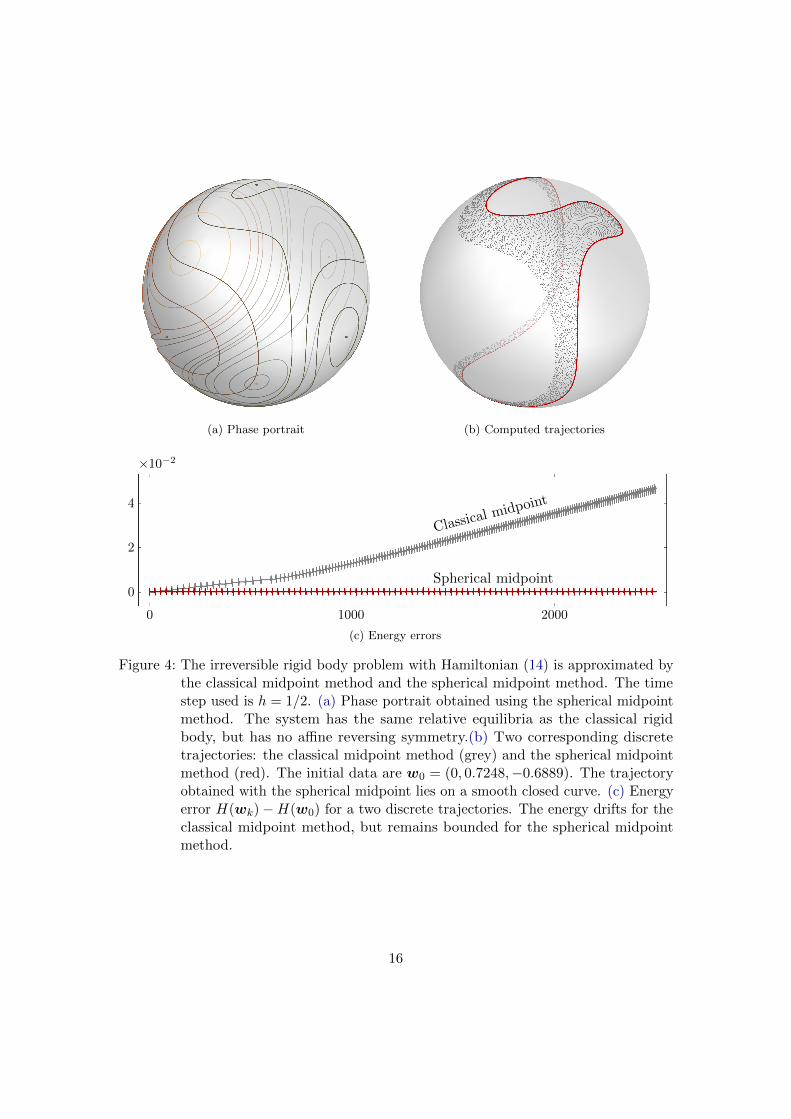
rotations are different. A phase portrait is given in Figure 4(a). Like the free rigidbody, the poles of the principal axes are relative equilibria, and every trajectory isperiodic. Contrary to the free rigid body, the phase portrait is not symmetric undercentral inversions, i.e., there is no apparent time-reversal symmetry.
We consider two different discrete approximations: the classical midpoint method (5)and the spherical midpoint method (3). Locally the two methods are akin (they areboth second order accurate), but they exhibit distinct global properties: trajectories lieon periodic curves for the spherical midpoint method but not for the classical midpointmethod; see Figure 4(b). Also, the deviation in the Hamiltonian (14) along discretetrajectories remains bounded for the spherical midpoint method, but drifts for theclassical midpoint method; see Figure 4(c).
Periodicity of phase trajectories and near conservation of energy, as displayed forthe spherical midpoint method, suggests the presence of a first integral, a modifiedHamiltonian, that is exactly preserved. The existence of such a modified Hamiltonianhinges on symplecticity, as established through the theory of backward error analysis [8].
The example in this section illustrates the advantage of the spherical midpoint method,over the classical midpoint method, for approximating Hamiltonian dynamics on S2. Ingeneral, one can expect that spherical midpoint discretisations of continuous integrablesystems on (S2)n remain almost integrable in the sense of Kolmogorov–Arnold–Mosertheory for symplectic maps, as developed by Shang [34].
3.3. Single particle system: forced rigid body, development of chaos
Consider the time dependent Hamiltonian on S2 given by
H(w, t) =1
2w · I−1w + ε sin(t)w3, w = (w1, w2, w3),
where I is an inertia tensor, given by
I =
I1 0 00 I2 00 0 I3
, I1 = 1, I2 = 4/3, I3 = 2.
This system describes a forced rigid body with periodic loading of period 2π. At ε = 0the system is integrable, but it becomes non-integrable as ε increases. We discretise thesystem using the spherical midpoint method with time-step length 2π/N , N = 20. APoincare section is obtain by sampling the system every N :th step; the result for variousinitial data and choices of ε is shown in Figure 5. Notice the development of chaoticbehaviour near the unstable equilibria points.
The example in this section illustrates that the spherical midpoint method, beingsymplectic, behaves as expected in the transition from integrable to chaotic dynamics.
3.4. 4–particle system: point vortex dynamics on the sphere
Point vortices constitute special solutions of the Euler fluid equations on two-dimensionalmanifolds; see the survey by Aref [1] and references therein. Consider the codimension
15
(a) Phase portrait (b) Computed trajectories
0 1000 2000
4
2
0
×10−2
Classical midpoint
Spherical midpoint
(c) Energy errors
Figure 4: The irreversible rigid body problem with Hamiltonian (14) is approximated bythe classical midpoint method and the spherical midpoint method. The timestep used is h = 1/2. (a) Phase portrait obtained using the spherical midpointmethod. The system has the same relative equilibria as the classical rigidbody, but has no affine reversing symmetry.(b) Two corresponding discretetrajectories: the classical midpoint method (grey) and the spherical midpointmethod (red). The initial data are w0 = (0, 0.7248,−0.6889). The trajectoryobtained with the spherical midpoint lies on a smooth closed curve. (c) Energyerror H(wk)−H(w0) for a two discrete trajectories. The energy drifts for theclassical midpoint method, but remains bounded for the spherical midpointmethod.
16

Figure 5: Poincare section of the forced rigid body system with Hamiltonian (3.3), ap-proximated by the spherical midpoint method. Left: ε = 0.01. Right: ε = 0.07.Notice the development of chaos near the unstable equilibria points.
zero submanifold of (S2)n given by
(S2)n∗ := {w ∈ (S2)n;wi 6= wj , 1 ≤ i < j ≤ n}.
Point vortex systems on the sphere, first studied by Bogomolov [3], are Hamiltoniansystems on (S2)n∗ that provide approximate models for atmosphere dynamics with localisedareas of high vorticity, such as cyclones on Earth and vortex streets [9] on Jupiter. Inabsence of rotational forces, the Hamiltonian function is given by
H(w) = − 1
4π
∑i<j
κiκj ln(2− 2wi ·wj).
In this context, the constants κi of the symplectic structure (1) are called vortex strengths.The cases n = 1, 2, 3 are integrable [12, 33], but the case n = 4 is non-integrable.Characterisation and stability of relative equilibria have been studied extensively; see [15]and references therein.
In this example, we study the case n = 4 and κi = 1 by using the time-discreteapproximation provided by the spherical midpoint method (3). Our study reveals a non-trivial 4-dimensional invariant manifold of periodic solutions.1 The invariant manifoldcontains both stable and non-stable equilibria.
First, let c(θ, φ) :=(
cos(φ) sin(θ), sin(θ) sin(φ), cos(θ))
and let
C(θ, φ) :=
c(θ, φ)
c(θ, φ+ π)c(π − θ,−φ)c(π − θ, π − φ)
.
1Interestingly, this special symmetric configuration was also found by Lim et al. [19]. We thank JamesMontaldi for pointing this out.
17

2θ
2θ
2φ
2φ
x1 x2
x3
x4
Figure 6: Illustration of the invariant submanifold I ⊂ (S2)4∗ given by (15).
Next, consider the two-dimensional submanifold of (S2)4∗ given by
I = {w ∈ (S2)4∗ ;w = C(θ, φ), θ ∈ [0, π), φ ∈ [0, 2π)}. (15)
See Figure 6 for an illustration.The numerical observation that I is an invariant manifold for the discrete spherical
midpoint discretisation led us to the following result for the continuous system.
Proposition 3.1.
I = {w ∈ (S2)4∗;w = A · w, A ∈ SO(3), w ∈ I}
is a 5–dimensional invariant manifold for the continuous 4–particle point vortex system onthe sphere with unitary vortex strengths. Furthermore, every trajectory on I is periodic.
Proof. Direct calculations show that XH is tangent to I. The result for I follows since His invariant with respect to the action of SO(3) on (S2)4.
The example in this section illustrates how numerical experiments with a discretesymplectic model can give insight to the corresponding continuous system. Generalisationof the result in Proposition 3.1 to other vortex ensembles is an interesting topic left forfuture studies.
3.5. n–particle system: Heisenberg spin chain
The classical Heisenberg spin chain of micromagnetics is a Hamiltonian system on (S2)n
with strengths κi = 1 and Hamiltonian
H(w) =
n∑i=1
wi−1 ·wi, w0 = wn. (16)
18

Figure 7: Particle trajectories on the invariant manifold I. The singular points aremarked in red (these points are not part of I). Notice that there are two typesof equilibria: the corners and the centres of the “triangle like” trajectories. Thecorners are unstable (bifurcation points) and the centres are stable (they are,in fact, stable on all of (S2)4
∗, as is explained in [15]).
For initial data distributed equidistantly on a closed curve, the system (16) is a spacediscrete approximation of the Landau–Lifshitz equation (see [14] for an overview). ThisPDE is known to be integrable, so one can expect quasiperiodic behaviour in the solution.Indeed, if we use the spherical midpoint method for (16), with n = 100 and initialdata equidistantly distributed on a closed curve, the resulting dynamics appear to bequasiperiodic (see Figure 8).
The example in this section illustrates that the spherical midpoint method, togetherwith a spatial discretisation, can be used to accurately capture the dynamics of integrableHamiltonian PDEs on S2.
A. Generalisation to Nambu systems
It is natural to ask for which non-canonical symplectic or Poisson manifolds other than(S2)n generating functions can be constructed. In full generality, this is an unsolvedproblem: no method is known to generate, for example, symplectic maps of a symplecticmanifold F−1({0}) in terms of F : T ∗Rd → Rk. In this appendix we shall show that thespherical midpoint method does generalise to Nambu mechanics [30]. Let C : R3 → Rbe a homogeneous quadratic function defining the Nambu system w = ∇C(w)×∇H(w)with Hamiltonian H ∈ C∞(R3). For C(w) = 1
2 |w|2, these are spin systems with a single
spin. The Lagrange system w1 = w2w3, w2 = w3w1, w3 = w1w2 is an example of aNambu system with C = 1
2(w21 − w2
2) and H = 12(w2
1 − w23).
19

Figure 8: Evolution of the Heisenberg spin chain system (16) with n = 100 for initialdata equidistantly spaced on a simple closed curve using the spherical midpointmethod. The corresponding Hamiltonian PDE (the Landau–Lifshitz equation)is known to be integrable.
Proposition A.1. A symplectic integrator for the symplectic manifold given by thelevel set C(w) = c 6= 0 in a Nambu system w = f = ∇C × ∇H, C = 1
2wTCw, is
given by the classical midpoint method applied to the Nambu system with HamiltonianH(w/
√C(w)/c).
Proof. The Poisson structure of the Nambu system is given byK(w)(σ, λ) = det([Cw, σ, λ]).Let X be the projected Nambu vector field. Calculations as in the proof of Theorem 2.4now give
K(W )(Σ,Λ)−K(w)(σ, λ) = h3 det([C−→w ,−→σ ,−→λ ]
= h3 det([CX(w),−DX(w)>σ,−DX(w)>λ]).
As before, all three arguments are orthogonal to w: CX(w), because X(w) is tan-gent to the level set C(w) = c, whose normal at w is Cw, and −DX(w)>σ because〈−DX(w)>σ,w〉 = 〈σ,−DX(w)w〉, and becausew 7→ H(w/
√C(w)/c) is homogeneous
on rays, X is constant on rays.
Note that if H is also a homogeneous quadratic (as in the Lagrange system), thenthe method preserves C and H and generates an integrable map. The Nambu systemsin Proposition A.1 are all 3-dimensional Lie–Poisson systems. There are 9 inequivalentfamilies of real irreducible 3-dimensional Lie algebras [31]. Five of them have homogeneousquadratic Casimirs and are covered by Proposition A.1: in the notation of [31], theyare A3,1 (C = w2
1, Heisenberg Lie algebra) A3,4 (C = w1w2, e(1, 1)); A3,6 (C = w21 + w2
2,e(2)); A3,8 (C = w2
2 + w1w3, su(1, 1), sl(2)); A3,9 (C = w21 + w2
2 + w23, su(2), so(3)). A
large set of Lie–Poisson systems is obtained by direct products of the duals of these Liealgebras. Such a structure was already mentioned by Nambu in his original paper, noting
20
the application to spin systems. The spherical midpoint method applies to these systems;it generates symplectic maps in neighbourhoods of symplectic leaves with c 6= 0.
References
[1] H. Aref, Point vortex dynamics: a classical mathematics playground, J. Math. Phys.48 (2007), 065401, 23.
[2] M. A. Austin, P. Krishnaprasad, and L.-S. Wang, Almost Poisson integration ofrigid body systems, Journal of Computational Physics 107 (1993), 105–117.
[3] V. Bogomolov, Dynamics of vorticity at a sphere, Fluid Dynamics 12 (1977), 863–870.
[4] P. Channell and J. Scovel, Integrators for Lie–Poisson dynamical systems, PhysicaD: Nonlinear Phenomena 50 (1991), 80 – 88.
[5] B. Chirikov and D. Shepelyansky, Chirikov standard map, Scholarpedia 3 (2008),3550.
[6] G. Cooper, Stability of Runge–Kutta methods for trajectory problems, IMA J.Numer. Anal. 7 (1987), 1–13.
[7] P. Deift, L.-C. Li, and C. Tomei, Loop groups, discrete versions of some classicalintegrable systems, and rank 2 extensions, vol. 100, AMS, 1992.
[8] E. Hairer, C. Lubich, and G. Wanner, Geometric Numerical Integration, Springer-Verlag, Berlin, 2006.
[9] T. Humphreys and P. S. Marcus, Vortex Street Dynamics: The Selection Mechanismfor the Areas and Locations of Jupiter’s Vortices, Journal of the Atmospheric Sciences64 (2007), 1318–1333.
[10] L. Jay, Symplectic partitioned Runge–Kutta methods for constrained Hamiltoniansystems, SIAM J. Numer. Anal. 33 (1996), 368–387.
[11] K. Kaneko and K. Kaneko, Theory and applications of coupled map lattices, vol. 159,Wiley Chichester, 1993.
[12] R. Kidambi and P. K. Newton, Motion of three point vortices on a sphere, PhysicaD: Nonlinear Phenomena 116 (1998), 143 – 175.
[13] Y. Kosmann-Schwarzbach, B. Grammaticos, and T. Tamizhmani, Discrete integrablesystems, Springer, 2004.
[14] M. Lakshmanan, The fascinating world of the Landau–Lifshitz–Gilbert equation: anoverview, Philosophical Transactions of the Royal Society A: Mathematical, Physicaland Engineering Sciences 369 (2011), 1280–1300.
21

[15] F. Laurent-Polz, J. Montaldi, and M. Roberts, Point vortices on the sphere: stabilityof symmetric relative equilibria, J. Geom. Mech. 3 (2011), 439–486.
[16] T. Lee, Can time be a discrete dynamical variable?, Physics Letters B 122 (1983),217 – 220.
[17] T. Lee, Difference equations and conservation laws, Journal of Statistical Physics46 (1987), 843–860.
[18] D. Lewis and N. Nigam, Geometric integration on spheres and some interestingapplications., J. Comput. Appl. Math. 151 (2003), 141–170.
[19] C. Lim, J. Montaldi, and M. Roberts, Relative equilibria of point vortices on thesphere, Phys. D 148 (2001), 97–135.
[20] C. Lubich, B. Walther, and B. Brugmann, Symplectic integration of post-Newtonianequations of motion with spin, Phys. Rev. D 81 (2010), 104025.
[21] J. Marsden and A. Weinstein, Coadjoint orbits, vortices, and Clebsch variables forincompressible fluids, Phys. D 7 (1983), 305–323.
[22] J. E. Marsden, S. Pekarsky, and S. Shkoller, Discrete Euler-Poincare and Lie–Poissonequations, Nonlinearity 12 (1999), 1647–1662.
[23] J. E. Marsden and T. S. Ratiu, Introduction to Mechanics and Symmetry, Springer-Verlag, New York, 1999.
[24] R. I. McLachlan, K. Modin, H. Z. Munthe-Kaas, and O. Verdier, B-series methodsare exactly the affine equivariant methods, Numerische Matematik (2015), http://arxiv.org/abs/1409.1019, 1409.1019.
[25] R. I. McLachlan, K. Modin, and O. Verdier, Collective symplectic integrators,Nonlinearity 27 (2014), 1525.
[26] R. I. McLachlan, K. Modin, and O. Verdier, Collective Lie–Poisson integrators onR3, IMA J. Num. Anal. 35 (2015), 546–560.
[27] R. I. McLachlan, K. Modin, O. Verdier, and M. Wilkins, Geometric generalisationsof SHAKE and RATTLE, Found. Comput. Math. 14 (2013), 339–370.
[28] R. I. McLachlan and G. R. W. Quispel, Geometric integrators for ODEs, Journal ofPhysics A: Mathematical and General 39 (2006), 5251.
[29] J. Moser and A. P. Veselov, Discrete versions of some classical integrable systemsand factorization of matrix polynomials, Comm. Math. Phys. 139 (1991), 217–243.
[30] Y. Nambu, Generalized Hamiltonian dynamics, Physical Review D 7 (1973), 2405–2412.
22

[31] J. Patera, R. Sharp, P. Winternitz, and H. Zassenhaus, Invariants of real lowdimension Lie algebras, Journal of Mathematical Physics 17 (1976), 986.
[32] H. Poincare, Les Methodes Nouvelles de la Mecanique Celeste, Gauthier–Villars,Paris, transl. in New Methods of Celestial Mechanics, Daniel Goroff, ed. (AIP Press,1993), 1892.
[33] T. Sakajo, The motion of three point vortices on a sphere, Japan Journal of Industrialand Applied Mathematics 16 (1999), 321–347.
[34] Z. Shang, KAM theorem of symplectic algorithms for Hamiltonian systems, Numer.Math. 83 (1999), 477–496.
[35] R. Steinigeweg and H.-J. Schmidt, Symplectic integrators for classical spin systems.,Comput. Phys. Commun. 174 (2006), 853–861.
[36] C. Viterbo, Generating functions, symplectic geometry, and applications, Proceedingsof the International Congress of Mathematicians, vol. 1, p. 2, 1994.
[37] A. Weinstein, Symplectic geometry, Bull. Amer. Math. Soc. (N.S.) 5 (1981), 1–13.
23