a minimal model for forest fire regimes

The University of Chicago

A Minimal Model for Forest Fire Regimes.Author(s): Renato Casagrandi and Sergio RinaldiSource: The American Naturalist, Vol. 153, No. 5 (May 1999), pp. 527-539Published by: The University of Chicago Press for The American Society of NaturalistsStable URL: http://www.jstor.org/stable/10.1086/303194 .

Accessed: 27/09/2014 04:28

Your use of the JSTOR archive indicates your acceptance of the Terms & Conditions of Use, available at .http://www.jstor.org/page/info/about/policies/terms.jsp

.JSTOR is a not-for-profit service that helps scholars, researchers, and students discover, use, and build upon a wide range ofcontent in a trusted digital archive. We use information technology and tools to increase productivity and facilitate new formsof scholarship. For more information about JSTOR, please contact [email protected].

.

The University of Chicago Press, The American Society of Naturalists, The University of Chicago arecollaborating with JSTOR to digitize, preserve and extend access to The American Naturalist.

http://www.jstor.org

This content downloaded from 68.168.203.75 on Sat, 27 Sep 2014 04:28:41 AMAll use subject to JSTOR Terms and Conditions

http://www.jstor.org/action/showPublisher?publisherCode=ucpress

http://www.jstor.org/action/showPublisher?publisherCode=amsocnat

http://www.jstor.org/stable/10.1086/303194?origin=JSTOR-pdf

http://www.jstor.org/page/info/about/policies/terms.jsp


vol. 153, no. 5 the american naturalist may 1999

A Minimal Model for Forest Fire Regimes

Renato Casagrandi1,* and Sergio Rinaldi2,†

1. Politecnico di Milano, Via Ponzio 34/5, 20133 Milano, Italy;2. CIRITA, Politecnico di Milano, Via Ponzio 34/5, 20133 Milano,Italy

Submitted April 15, 1998; Accepted November 25, 1998

abstract: We show in this article how the characteristics of firerecurrence in forests can be theoretically derived from simple infor-mation concerning forest morphology. The task is accomplished bymeans of a minimal model encapsulating a few assumptions on theinteractions between overstory and understory species and on themechanisms of fire development and transmission. The main dif-ference with other models for fire prediction and simulation is that,here, fire is an endogenous variable with purely deterministic dy-namics. Nevertheless, the analysis shows that fire recurrence can bechaotic for parameter values corresponding to Mediterranean forests.By contrast, the model shows that boreal forests and savannas havethe tendency to experience periodic fires. These general results arein agreement with the studies carried out on many different forestsin this century.

Keywords: forest fires, Mediterranean forests, savannas, boreal forests,cycles, chaos.

Forests can be classified in different ways depending onthe characteristics one likes to focus on. Four importantgroups are present in many, if not all, classifications (Spurr1964; Walter 1985; Archibold 1995): rain forests, borealforests, savannas, and Mediterranean forests. The defini-tion of each class is usually based on forest morphology.Rain forests are dense and humid, and layers are not easilyrecognizable (Longman and Jenık 1974; Richards 1996).Boreal forests are characterized by high density of largeconifers and scarcity of bush (Viereck et al. 1983), theprevalent understory species being bryophytes and lichens(Johnson 1981). By contrast, trees are quite rare whileherbs are very dense in savannas (Menaut and Cesar 1979;Huntley and Walker 1982). Finally, in Mediterranean for-

* E-mail: [email protected].

† E-mail: [email protected].

Am. Nat. 1999. Vol. 153, pp. 527–539. q 1999 by The University of Chicago.0003-0147/99/5305-0006$03.00. All rights reserved.

ests, both understory and overstory species are important(di Castri and Mooney 1973). The same classification issometimes based on different arguments, like the char-acteristics of fire regimes. Indeed, fires are only accidentalin rain forests (Sanford et al. 1985; Saldarriaga and West1986), while they are recurrent in other forests. But fireregimes of boreal forests, savannas, and Mediterraneanforests are remarkably different. Indeed, fires in northernboreal forests prevalently involve crowns (Kasischke et al.1995), and the fire return times are typically 50–200 yr(Rowe and Scotter 1973; Zackrisson 1977; Engelmark1984; Payette 1989). By contrast, fires in savannas are sur-face fires, and return times are typically 1–2 yr in moistsavannas (Scott 1971; Goldammer 1983) and 5–10 yr inarid savannas (Tyson and Dyer 1975; Rutherford 1981).Finally, in Mediterranean forests, fires can be either crownor surface fires and occur in an apparently random se-quence. This diversity gives rise to a pronounced variabilityof the fire return times (10–100 yr as reported by Kruger[1983] and Davis and Burrows [1994]). Thus, the varia-bility of the return time at a given site is not very pro-nounced in boreal forests (see Bonan 1989 and referencestherein) and savannas (see Goldammer 1983 and refer-ences therein), while it is in Mediterranean forests (Kruger1983). By oversimplifying a bit the overall picture, onecould say that fires are absent in rain forests, periodic atlow frequency in boreal forests, periodic at high frequencyin savannas, and recurrent but aperiodic in Mediterraneanforests.

Thus, the same classification can be obtained in twodifferent ways, namely, by looking at forest morphologyor at fire regimes. While it is true that savannas are “trop-ical formations where the grass stratum is continuous andimportant but occasionally interrupted by trees and shrubs[and] the stratum is burnt from time to time” (Bourliereand Hadley 1970, pp. 125–126), it is also true that sucha definition contains some redundancy because, as shownin this article, the morphology of a given forest identifiesits fire regime. Although this is a priori more than con-ceivable, we are not aware of any formal theoretical der-ivation of such a property. For this reason, we show inthis article how this property can be derived from a simplebut general model based only on standard assumptions on



528 The American Naturalist

the interactions between overstory and understory speciesand on the mechanisms of fire development and trans-mission. The model can be viewed as a classical ecologicalmodel composed of two predators (crown and surfacefires) and two preys (overstory and understory species).Of course, other analogies, for example, with epidemics,could also be explored, as suggested by an anonymousreviewer. The model is purely deterministic and shouldnot be confused or compared with the numerous sto-chastic models for fire prediction (see, e.g., Van Wagner1978; Johnson and Van Wagner 1985; Davis and Burrows1994; Chao et al. 1997). In the model, the forest is idealizedas two homogeneous, interacting layers called upper (u)and lower (l) layers. Each layer is composed of two com-partments, the green (G) and the red (R) biomass, thesecond one identifying the burning biomass. The dynamicbehavior of the model is studied through bifurcation anal-ysis, and the result is surprisingly neat. It shows that de-pending on the value of some strategic parameters theforest can behave in four possible ways corresponding,indeed, to the four distinct fire regimes outlined above.The conclusion is that the assumptions we have encap-sulated in our simple model have the power of explainingthe fire regimes of rain forests, boreal forests, savannas,and Mediterranean forests.

A Minimal Model

We now describe the model on which our analysis is based.It is such a crude simplification of reality that the word“model” is almost inappropriate. Indeed, models that ne-glect many of the mechanisms that are known to operatein the field are sometimes called “minimal” in order todistinguish them from detailed simulation models. Min-imal models are based only on a few basic facts that arerelated to the property one would like to discuss. In gen-eral, simulation models are tuned on a specific forest, whileminimal models are used to characterize and classify thebehaviors (e.g., the fire regimes) of large classes of forests.

The identification and the classification of all modes ofbehavior of a model requires a paramount effort if themodel is complex, that is, if it has more than a few variablesand parameters. Spatial heterogeneity is systematicallyruled out in minimal models because it would require usto work with partial differential equations or with a greatnumber of ordinary differential equations, thus makingthe problem intractable. For the same reason, species di-versity, age structure, and plant physiology are also notconsidered, unless they are strategically important. Thus,in our minimal model, we look only at total biomass (see,e.g., Shugart 1984, chap. 6), but in order to distinguishcrown fires from surface fires, we consider an upper veg-etational layer, in general composed of trees of various

species, and a lower vegetational layer that, depending onthe forest, is composed of bryophytes, herbs, shrubs, orany mix of these plants.

At time t, a tree (or a part of it) is either burning ornot burning so that the biomass of the upper layer canbe subdivided into green component, indicated by ,G (t)u

and red component, indicated by . Similarly, the bi-R (t)u

omass of the lower layer is subdivided into green biomassand red biomass . Obviously, and areG (t) R (t) R (t) R (t)l l u l

indicators of fire intensity in the two layers at time t.The instantaneous rate of variation of each biomass can

be specified through a simple mass balance equation. Inparticular, the rate of variation of the green biomass ofeach layer is the difference between a growthG 5 dG/dtrate g (taking into account productivity, natural mortality,and competition) and the rate f at which green biomassis attacked by fire. Since fire transforms green biomassinto red biomass, the rate of variation of theR 5 dR/dtred biomass of each layer is the difference between f andthe rate e at which such a biomass goes extinct.

Thus, the minimal model is a fourth-order continuous-time model of the form

G 5 g 2 f , (1)u u u

R 5 f 2 e , (2)u u u

G 5 g 2 f , (3)l l l

R 5 f 2 e , (4)l l l

where the first two equations describe the upper layer, andthe last two the lower layer.

In order to specify the model, we must first define thearguments of the functions e, f, and g. Of course, this mustbe done by trading off between two conflicting objectives:the realism of the model and its simplicity. We assumethat the combustion processes of burning plants are notinfluenced by the surrounding green biomasses, that is,

e 5 e (R ),u u u

e 5 e (R ),l l l

while for fire ignition rates, we write

f 5 f (G , R , R ),u u u u l

f 5 f (G , R , R ),l l l u l

because the burning biomass of each layer attacks the greenbiomasses of both layers. Finally, shadowing and com-petition for nutrients among plants of different layers im-ply that both growth rates and depend on, in principle,g gu l



A Model for Forest Fire Regimes 529

Figure 1: Influence graph of the minimal model (A) and Vandermeer’smodel (B). Both models can be interpreted as two coupled oscillators:in case A each layer can be an oscillator, while in case B each prey-predator pair can be an oscillator.

the green biomasses of both layers. Nevertheless, in thefollowing, we consider the asymmetric case

g 5 g (G ),u u u

g 5 g (G , G ),l l u l

g l! 0,

Gu

corresponding to forests in which interlayer competitionfor nutrients is negligible and understory species are neg-atively influenced by shadowing.

The structure of the model is described by the influencegraph of figure 1A, which shows that each layer can beinterpreted as a prey-predator assembly, where the prey isthe green biomass and the predator the red one. As is wellknown (May 1976), such an assembly can be an oscillator(biological clock) even in the absence of external forcing(environmental clock). In other words, for suitable func-tions e, f, and g, each single layer of our model can ex-perience periodic fires, even in the absence of seasons.Thus, the model is composed of two coupled oscillators.The literature on this topic is very rich (see Strogatz 1994).It is rooted in a study of Huygens, who in the seventeenthcentury discovered that two asynchronous clocks couldlock their frequencies when they were hanging on the samewall. But frequency locking is only one of the many com-plex and intriguing behaviors (including deterministicchaos) that can occur when coupling nonlinear oscillators(Guckenheimer and Holmes 1983). In the ecological con-text, coupled oscillators have been used by Vandermeer(1993) to explain the complex dynamics of communitiescomposed of two populations preyed on by two predatorpopulations. But the influence graph of Vandermeer’smodel (see fig. 1B) is radically different from that of ourmodel. In fact, fire transmission between layers corre-sponds to a beneficial influence between predators, a factusually not present in other ecosystems where differentpredators do not interact or interact negatively throughinterference. In conclusion, even if our model is composedof two prey-predator submodels, the coupling is not stan-dard, and the results obtained by Vandermeer cannot beused to predict the fire regimes. In other words, our min-imal model is a new model and must be studied per se.

In order to further specify the model, we must decidehow to deal with environmental (weather) variability. Forthis we can distinguish between (1-yr) periodic determin-istic components, identified by a standard season, andaperiodic stochastic components, that is, deviations fromthe standard season (like storms, windy summers, severedroughts, etc.). In principle, the deterministic componentcould be included in the model by assuming that some

parameters (e.g., fire transmission and extinction rates)are periodically varying with period of 1 yr. But this is notreally needed in the present case because the existing con-tributions on periodically forced predator-prey models(Hastings et al. 1993; Rinaldi et al. 1993) show that theinteractions between biological and environmental clocksare relevant only if the frequencies of the two clocks arenot too different. Since this condition is not satisfied inMediterranean and boreal forests (where the environmen-tal and biological frequencies are in the ratio1 : 20–1 : 200), the use of a constant parameter model forsuch forests is justified. On the other hand, seasonalitiesare moderate at the Tropics, so that the choice of a constantparameter model seems a natural one also for savannas.By contrast, stochastic variability certainly plays an im-portant role because it deals with rare but severe episodesthat can anticipate or delay fires with respect to those that




Table 1: Vegetational data

Forest type

NPP Biomass

Min Max Min Max

Rain 1 3.5 6 80Boreal .4 2 6 40Savanna .2 2 .2 15Mediterranean .5 1.5 .7 26

Note: Minimum (min) and maximum (max) values

of net primary productivity (NPP) and biomass are

expressed in and , respectively.22 21 22kg m yr kg m

Data for rain forests, boreal forests, and savannas are

derived from Whittaker and Woodwell (1971) and

Whittaker and Likens (1975), while data for Mediter-

ranean forests are taken from Lieth (1975), De Bano

and Conrad (1978), Hoffmann and Kummerow

(1980), and Malanson and Trabaud (1987).

would occur in standard conditions. Nevertheless, sto-chastic variability will be intentionally omitted because wewant to show that some forests would experience recurrentaperiodic fires even in a constant environment. In otherwords, our thesis is that nonlinear biological interactionscan be the source of complex fire regimes and that sucha complexity can possibly be reinforced by weatherstochasticity.

The analysis will not be carried out in general but fora significant class of the functions e, f, and g giving riseto the following model:

GuG 5 r G 1 2u u u( )k u

Gu2b R (5)u uG 1 hu uu

Gu2 g R ,u lG 1 hu ul

GuR 5 b Ru u uG 1 hu uu

Gu1 g R 2 d R , (6)u l u uG 1 hu ul

G lG 5 r G 1 2 2 aG Gl l l u l( )k l

G l2 b R (7)l lG 1 hl ll

G l2 g R ,l uG 1 hl lu

G lR 5 b Rl l lG 1 hl ll

G l1 g R 2 d R . (8)l u l lG 1 hl lu

In equations (5)–(8), all parameters are indicated by low-ercase letters and are constant in time, while the four statevariables are indicated by capital letters. In the absence offire ( ), trees grow 1ogistically toward the car-R 5 R 5 0u l

rying capacity (see eq. [5]). By contrast, plants of thek u

lower layer do not tend toward their carrying capacitybecause tree canopy reduces light availability. This hask l

been taken into account by introducing a mortality rateproportional to into equation (7). Thus, if there is noGu

fire and trees tend toward their carrying capacity, the greenbiomass of the lower layer tends toward . The(1 2 ak /r )ku l l

fire attack rates and appearing in equations (1)–(4)f fu l

are the sum of two components representing the fire at-tacks due to the burning biomasses of the two layers. Eachcomponent is proportional to the product of a burningbiomass R and the probability P that such a red biomasstransmits fire to the green biomass G. Obviously P in-creases with green biomass, it is equal to 0 for andG 5 0saturates to 1 for G tending to infinity. Functions of thiskind are the Monod function and Ivlev’sP 5 G/(G 1 h)function . In equations (5)–(8), we have used2aGP 5 1 2 ethe Monod function that is more popular in the contextof predator-prey models, but we have checked that theresults of our analysis are not influenced practically by thischoice. The parameter h appearing in the Monod function(called half-saturation constant) is the density of greenbiomass at which the fire transmission rate of the burningbiomass is half maximum. The maximum fire attack rateswithin the same layer are denoted by b, while the interlayerfire attack rates are denoted by g. Finally, as for the func-tions e, the parameters d in equations (6) and (8) representthe rate at which burning trees and burning plants of thelower layer become extinct. In the extinction phase of asevere fire, when is negligible, equation (6) becomesGu

so that exp( ). In otherR 5 2d R R (t) 5 R (0) 2d tu u u u u u

words, crown fires decay exponentially with a time con-stant 1/ . Similarly, surface fires decay exponentially withdu

a time constant 1/ .d l

Model (5)–(8) has 15 parameters. Five of them( ) specify vegetation growth in the two layers,r , k , r , k , au u l l

while the others are related to fire characteristics. In orderto adapt the model to different classes of forests, the pa-rameters must be assigned properly. Many parametersmust have extreme values in savannas and boreal forestsbecause in these forests one of the two layers is muchmore dense than the other. Table 1 reports the net primaryproductivity ranges and the biomass ranges, and table 2




Table 2: Vegetational and fire parameters

Units Minimum Maximum

ru yr21 .05 (b) 1 (s)rl yr21 . 1 (b) 4 (s)ku 10 22kg m .15 (s) 3 (b)k l 10 22kg m .05 (b) 3 (r)a .1 2 21 21m kg yr .003 (b) 16 (s)bu yr21 18 (b) 50 (s)bl yr21 20 (b) 90 (s)du yr21 15 (b) 60 (s)dl yr21 25 (b) 75 (s)gu yr21 .01 (b) 5 (r)gl yr21 .01 (b) 5 (r)huu 10 22kg m .0015 (s) .15 (b)hul 10 22kg m .0015 (s) .15 (b)h ll 10 22kg m .0005 (b) .15 (r)h lu 10 22kg m .0005 (b) .15 (r)

Note: Ranges of vegetational and fire parameters used in

the model. The type of forest ( , ,r 5 rain b 5 boreal s 5

) corresponding to extreme parameter values is in-savanna

dicated in parentheses.

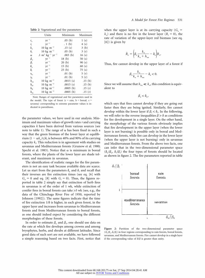
Figure 2: Partition of the two-dimensional parameter space( ) in four regions corresponding to rain forests, boreal forests,d /b , d /bu u l l

savannas, and Mediterranean forests. Fire cannot develop in a single layerif the corresponding value of is greater than unity.d/b

the parameter values, we have used in our analysis. Min-imum and maximum values of growth rates r and carryingcapacities k have been derived from various sources (seenote to table 1). The range of a has been fixed in such away that the green biomass of the lower layer at equilib-rium is between 40% and 90% of its carrying(1 2 ak /r )ku l l

capacity . This reduction is in agreement with studies onk l

savannas and Mediterranean forests (Grunow et al. 1980;Specht et al. 1983). Notice that a is minimum in borealforests, where the plants of the lower layer are shade tol-erant, and maximum in savannas.

The identification of realistic ranges for the fire param-eters is not an easy task because available data are scarce.Let us start from the parameters and and recall thatd du l

their inverses are fire extinction times (see eq. [6] withand eq. [8] with ). Thus, the figures re-G 5 0 G 5 0u l

ported in table 2 simply say that extinction of herb firesin savannas is of the order of 1 wk, while extinction ofconifer fires in boreal forests can take 13 wk (see, e.g., thedata of the Chinchaga River Fire of 1950, reported byJohnson [1992]). The same figures indicate that the timeof fire extinction 1/d is higher, in each given forest, in theupper layer and increases from savannas to Mediterraneanforests and from Mediterranean forests to boreal forests,as one should indeed expect by considering the differentmorphologies of these forests.

In order to estimate and , one should use data onb bu l

the rate at which fire develops among crowns and amongbryophytes, herbs, and shrubs at different latitudes. Sincegood data of such sort are not available, we have followeda simple reasoning based on two facts. First, notice that

when the upper layer is at its carrying capacity (G 5u

) and there is no fire in the lower layer ( ), thek R 5 0u l

rate of variation of the upper-layer red biomass (see eq.[6]) is given by

k uR 5 b 2 d R .u u u u( )k 1 hu uu

Thus, fire cannot develop in the upper layer of a forest if

k ub 2 d ! 0.u uk 1 hu uu

Since we will assume that , this condition is equiv-h K kuu u

alent to

b ! d ,u u

which says that fires cannot develop if they are going outfaster then they are being ignited. Similarly, fire cannotdevelop within the lower layer if . In the following,b ! dl l

we will refer to the reverse inequalities as conditionsb 1 d

for fire development in a single layer. On the other hand,the morphology of the various forests obviously impliesthat fire development in the upper layer (when the lowerlayer is not burning) is possible only in boreal and Med-iterranean forests, while fire can develop in the lower layer(when the upper layer is not burning) only in savannasand Mediterranean forests. From the above two facts, onecan infer that in the two-dimensional parameter space( , ) the four types of forests should be locatedd /b d /bu u l l

as shown in figure 2. The fire parameters reported in table




Figure 3: Transients of green biomasses as predicted by the minimal model for a rain forest after an accidental fire. Parameter values are r 5u

, , , , , , , , and . The dot on the left border of0.15 r 5 0.25 k 5 2 k 5 3 a 5 0.07 b 5 b 5 23 g 5 g 5 5 d 5 d 5 30 h 5 h 5 h 5 h 5 0.045l u l u l u l u l uu ul lu ll

the figure indicates initial conditions (see text).

2 are in agreement with figure 2 and show that the highestrate of fire development ( ) in a single layer is thatb 2 d

of the lower layer in savannas.The two parameters and are coupling parametersg gu l

(in fact, if were equal to 0, the upper layer would begu

fully independent of the lower layer). Interlayer fire trans-mission is rather small since the inflammable parts of thetwo layers are often quite separated in space. For thisreason, we have chosen and .g K b g K bu u l l

Finally, the half-saturation constants and haveh huu ul

been fixed between 1% and 5% of the carrying capacity, thus implying that crown fires develop at least at 90%k u

of their maximum speeds ( and ), even in forests thatb gu u

are at 50% of their upper-layer carrying capacity, since

k /2u 5 0.90.k /2 1 0.05ku u

The same criterion has been used to fix the ratios of h ll

and to . With this choice, the half-saturation constantsh klu l

have practically no role during severe fires but inhibit theoccurrence of fires in immature forests.

Model Behavior

In this section, we show how model (5)–(8) behaves forfour different parameter settings, corresponding to a typ-ical rain forest, boreal forest, savanna, and Mediterraneanforest, respectively.

Rain Forests

In order to determine the parameter setting of a rain forest,we first fix the values of , and in such a wayb , b , d du l u l

that the point ( , ) falls in the region indicatedd /b d /bu u l l

by “rain forest” in figure 2. Since upper and lower layerscan hardly be distinguished in rain forests, we have usedfor them the same parameter values andb 5 b 5 23u l

. The other parameter values have been se-d 5 d 5 30u l

lected within the ranges indicated in table 2, far from theextreme values that are typical of boreal forests and sa-vannas. Simulations of model (5)–(8) performed with ran-domly selected initial conditions show that the forest tendstoward the same equilibrium independently of initial con-ditions. Figure 3 reports the time patterns of green bio-masses as predicted by the model starting from the fol-lowing initial conditions

1G (0) 5 G (0) 5 k 5 1,u l u2

1R (0) 5 R (0) 5 k 5 0.2.u l u10

The patterns of red biomasses are not shown in the figurebecause they are !1023 ( ) after a few weeks, while22kg mgreen biomasses tend toward a plateau. The time neededto reach the equilibrium is of the order of 70 yr for bothlayers. Similar transients are obtained from different initialconditions, and the conclusion is that such a forest tendstoward a steady state in which fire is absent. Assumingthat this example is a good representative of rain forests,we could conclude that the minimal model explains why




Figure 4: Cyclical patterns of green biomasses as predicted by the minimal model for a boreal forest. Parameter values are , ,r 5 0.1 r 5 0.3u l

, , , , , , , , , , and .k 5 3 k 5 0.1 a 5 0.045 b 5 18 b 5 20 g 5 0.1 g 5 0.02 d 5 16.5 d 5 21 h 5 h 5 0.045 h 5 h 5 0.0015u l u l u l u l uu ul ll lu

fires can be ignited only by extremely severe (and hencerare) hazards.

Boreal Forests

In agreement with figure 2, one example of boreal foresthas been obtained by letting , , ,b 5 18 b 5 20 d 5 16.5u l u

and so that and , while thed 5 21 d /b ! 1 d /b 1 1l u u l l

remaining parameters have been fixed in accordance withtable 2. Simulations of model (5)–(8) show that the foresttends toward the same cyclical behavior independent ofthe initial conditions. Figure 4, which is in agreement withmany data and studies on boreal forests at high latitudes,shows the cyclical patterns of the green biomasses of theupper and lower layer (parameter values are reported inthe legend). The patterns of the red biomasses identifyingthe fires cannot be shown at the scale of the figure: theycorrespond to impulses with a return time of about 100yr (the so-called fire frequency; Yarie 1981). Actually, inthe simulations, the red biomass remains very low (i.e.,of the order of ) during most of the220 23 2210 2 10 [kg m ]cycle and then jumps to very high values for a few months,during which the green biomass of the lower layer is re-duced only by 50% (as indicated in Kasischke et al. 1995).After a fire, the green biomass of the lower layer increasesfor 20–30 yr (while conifers, which grow very slowly, arestill almost absent) and then decreases and reaches theprefire level within 60–100 yr, as theorized by Viereck(1983). Finally, when the upper-layer green biomassreaches a threshold, a new devastating crown fire veryquickly develops. In conclusion, the cycle is set up by theupper layer, while the lower layer (which, as a single layer,

would not experience recurrent fires because ) isd /b 1 1l l

simply entrained in the fire cycle (Engelmark 1987).It is worth noticing that some boreal forests experience

recurrent surface fires due to litter accumulation on theground (Kilgore and Taylor 1979). Obviously, such kindof fire cannot be explained by model (5)–(8), which doesnot account for litter. It is also important to remark thatthe fire regime predicted by the minimal model is rigor-ously periodic, while in reality the fire return time hassome variability. An obvious remedy for this would be toadd to equations (6) and (8) a suitable noise interpretingthe randomness of environmental factors facilitating firedevelopment. But this would be somehow against the spiritthat supports minimal models and would, indeed, hidethe crude but clear message of our study: the fire returntime of a boreal forest is constant and due to the endog-enous mechanisms of growth and interactions amonglayers.

Savannas

The case of savannas is somehow opposite to that of borealforests because the upper layer cannot experience, as asingle layer, recurrent fires while the lower layer, mainlycomposed by herbs, can. The selected parameter valuesare , , , and so thatb 5 50 b 5 80 d 5 53 d 5 72u l u l

and (see fig. 2), while the remainingd /b 1 1 d /b ! 1u u l l

parameters are in agreement with table 2. Figure 5 showsthe fire cycle that is, again, periodic but at high frequency(fire return time of about 5 yr, as in Gill 1975; Birk andSimpson 1980; Rutherford 1981). The cycle is set up bythe lower layer, and in fact the fire is a surface fire dev-astating the herbs (the loss in this layer is 90% of the




Figure 5: Cyclical patterns of green biomasses as predicted by the minimal model for a savanna. Parameter values are , , ,r 5 0.8 r 5 2.0 k 5 0.5u l u

, , , , , , , , and .k 5 0.4 a 5 2 b 5 50 b 5 80 g 5 g 5 1 d 5 53 d 5 72 h 5 h 5 0.0075 h 5 h 5 0.006l u l u l u l uu ul ll lu

Figure 6: Chaotic behavior of a Mediterranean forest: the fire return time varies randomly, as well as the peaks of green biomasses. Parametervalues are , , , , , , , and .r 5 0.25 r 5 1.5 k 5 k 5 1 a 5 0.5 b 5 b 5 25 g 5 g 5 0.1 d 5 d 5 21.25 h 5 h 5 h 5 h 5 0.015u l u l u l u l u l uu ul lu ll

prefire biomass), while tree biomass remains almost con-stant (the loss in this layer is less than 10%, as observedby Hopkins [1965]).

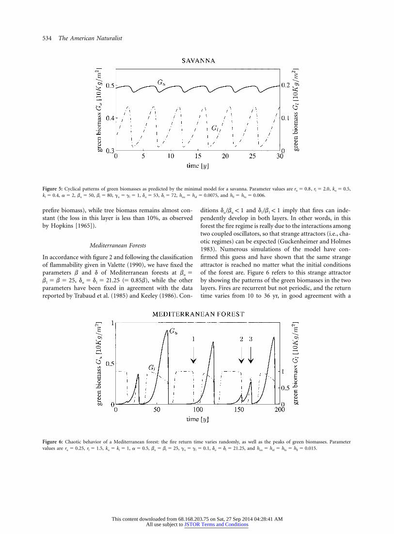
Mediterranean Forests

In accordance with figure 2 and following the classificationof flammability given in Valette (1990), we have fixed theparameters b and d of Mediterranean forests at b 5u

, , while the otherb 5 b 5 25 d 5 d 5 21.25 (5 0.85b)l u l

parameters have been fixed in agreement with the datareported by Trabaud et al. (1985) and Keeley (1986). Con-

ditions and imply that fires can inde-d /b ! 1 d /b ! 1u u l l

pendently develop in both layers. In other words, in thisforest the fire regime is really due to the interactions amongtwo coupled oscillators, so that strange attractors (i.e., cha-otic regimes) can be expected (Guckenheimer and Holmes1983). Numerous simulations of the model have con-firmed this guess and have shown that the same strangeattractor is reached no matter what the initial conditionsof the forest are. Figure 6 refers to this strange attractorby showing the patterns of the green biomasses in the twolayers. Fires are recurrent but not periodic, and the returntime varies from 10 to 36 yr, in good agreement with a




Figure 7: Two postfire recovery diagrams: graph A is obtained from theminimal model, by plotting the data of figure 6 (years 95–120); graphB is taken from Specht and Morgan (1981) and refers to an Australianforest.

number of studies (see, e.g., Hanes 1971; Le Houerou1974; Keeley 1977; Schlesinger and Gill 1978; Horne 1981).Three types of fires can be identified: surface fires (fig. 6,point 1) characterized by a very small reduction of treebiomass; mixed fires (fig. 6, point 2) characterized by amore important, but not devastating, impact on tree bi-omass; and crown fires (fig. 6, point 3) characterized bya severe depletion of tree biomass.

After a fire, the shrub biomass first increases but thendecreases when tree canopy intercepts light, in agreementwith Schlesinger and Gill (1980) and Trabaud (1994). Thiscan be put into better evidence by a postfire recoverydiagram obtained by plotting versus in the pe-G (t) G (t)l u

riod between two successive fires. This is done in figure7A using the data from year 95 to year 120 of figure 6and in figure 7B for an Australian forest (see Specht andMorgan 1981).

Robustness of the Results

We have shown in the previous section that the fire regimeof a forest is a consequence of its morphology. But theresult has been obtained by analyzing only one particularcase for each type of forest and needs, therefore, to befurther validated. In other words, we must verify the ro-bustness of our findings. The proper tool for this is bi-furcation analysis (Kuznetsov 1995), a technique used toidentify and to classify all possible modes of behavior (theso-called attractors) of a given dynamical system in spec-ified parameter ranges.

For the ease of the reader, we now briefly describe whatbifurcation analysis is about and how it can be performedin practice. Since model (5)–(8) has four differential equa-tions, its attractors (as well as its saddles and repellors)can be equilibria and limit cycles, as in second-order sys-tems, but also strange attractors (as we have seen in theprevious section). Each parameter setting corresponds toone model of our family (5)–(8) and, therefore, to onespecific set of attractors, saddles, and repellors. If one pa-rameter is slightly perturbed, by continuity the positionand the form of the attractors, saddles, and repellors instate space will vary smoothly (e.g., a cycle might becomeslightly bigger and faster) but all trajectories will remaintopologically the same (e.g., an attracting cycle will remainan attracting cycle). Only at some particular points inparameter space will the above continuity argument fail.At these points, called bifurcation points, small variationsof the parameters entail significant changes in model be-havior. For example, an equilibrium can be stable (i.e.,attract all nearby trajectories) for a given parameter settingbut lose its stability if one parameter is varied even of aninfinitesimal amount. If this is the case, for the new pa-rameter value the state of the system will not tend toward

the equilibrium but toward another attractor. In two-dimensional parameter spaces, bifurcation points identifythe so-called bifurcation curves, and these curves partitionthe parameter space into subregions. All the models cor-responding to the same subregion have the same quali-tative behavior because they have topologically equivalenttrajectories. Thus, if we want to produce a complete catalogof the modes of behavior of a system, we must simplydetermine all its bifurcation curves. This can be done byusing specialized software implementing continuationtechniques to carry out the computations (Khibnik et al.1993; Kuznetsov 1995). Once a bifurcation point in theparameter space is found, this software produces the entirebifurcation curve passing through that point.

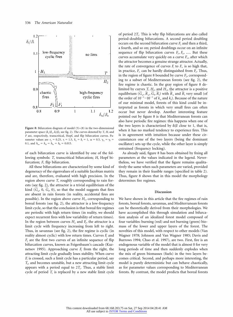
Without going into more details, we show the resultsof this analysis in figure 8, where the two parameters arethe nondimensional parameters and used ind /b d /bu u l l

figure 2 to classify forests. All other parameters are fixedat the values indicated in the legend to figure 8. The nature




Figure 8: Bifurcation diagram of model (5)–(8) in the two-dimensionalparameter space ( ; see fig. 2). The curves denoted by T, H, andd /b , d /bu u l l

F are, respectively, transcritical, Hopf, and flip bifurcation curves. Pa-rameter values are , , , ,r 5 0.25 r 5 1.5 k 5 k 5 1 a 5 0.5 g 5 g 5u l u l u l

, and .0.1 h 5 h 5 h 5 h 5 0.015uu ul lu ll

of each bifurcation curve is identified by one of the fol-lowing symbols: T, transcritical bifurcation; H, Hopf bi-furcation; F, flip bifurcation.

All these bifurcations are characterized by some kind ofdegeneracy of the eigenvalues of a suitable Jacobian matrixand are, therefore, evaluated with high precision. In theregion above curve T, roughly corresponding to rain for-ests (see fig. 2), the attractor is a trivial equilibrium of thekind ( , 0, , 0), so that the model suggests that firesG Gu l

are absent in rain forests (in reality, accidental fires arepossible). In the region above curve , corresponding toH1

boreal forests (see fig. 2), the attractor is a low-frequencylimit cycle, so that the conclusion is that boreal fire regimesare periodic with high return times (in reality, we shouldexpect recurrent fires with low variability of return times).In the region between curves and , the attractor is aH F2 1

limit cycle with frequency increasing from left to right.Thus, in savannas (see fig. 2), the fire regime is cyclic (inreality almost cyclic) with low return times. Curves andF1

are the first two curves of an infinite sequence of flipF2

bifurcation curves, known as Feigenbaum’s cascade (Kuz-netsov 1995). Approaching curve from the right, theF1

attracting limit cycle gradually loses stability. When curveis crossed, such a limit cycle has a particular period, sayF1

, and becomes unstable, but a new attracting limit cycleT1

appears with a period equal to 2 . Thus, a stable limitT1

cycle of period is replaced by a new stable limit cycleT1

of period 2 . This is why flip bifurcations are also calledT1

period-doubling bifurcations. A second period doublingoccurs on the second bifurcation curve and then a third,F2

a fourth, and so on; period doublings occur on an infinitesequence of flip bifurcation curves . But theseF , F , )3 4

curves accumulate very quickly on a curve , after whichF`

the attractor becomes a genuine strange attractor. Actually,the rate of convergence of curves to is so high that,F Fi `

in practice, can be hardly distinguished from . Thus,F F` 2

in the region of figure 8 bounded by curve , correspond-F2

ing to a subset of Mediterranean forests (see fig. 2), thefire regime is chaotic. In the gray region of figure 8 de-limited by curves T, , and , the attractor is a positiveH H1 2

equilibrium ( ) with and very small (ofG , R , G , R R Ru u l l u l

the order of 10 of and ). Because of the nature23 25210 k ku l

of our minimal model, forests of this kind could be in-terpreted as forests in which very small fires can oftenoccur but never develop. Another interesting featurepointed out by figure 8 is that Mediterranean forests canalso have periodic fire regimes: this happens when one ofthe two layers is characterized by close to 1, that is,d/bwhen it has no marked tendency to experience fires. Thisis in agreement with intuition because under these cir-cumstances one of the two layers (being the dominantoscillator) sets up the cycle, while the other layer is simplyentrained (frequency locking).

As already said, figure 8 has been obtained by fixing allparameters at the values indicated in the legend. Never-theless, we have verified that the figure remains qualita-tively the same when such parameters are varied, providedthey remain in their feasible ranges (specified in table 2).Thus, figure 8 shows that in this model the morphologydetermines fire regimes.

Discussion

We have shown in this article that the fire regimes of rainforests, boreal forests, savannas, and Mediterranean forestscan be theoretically derived from their morphologies. Wehave accomplished this through simulation and bifurca-tion analysis of an idealized forest model composed offour variables: burning (red) and not burning (green) bio-mass of the lower and upper layers of the forest. Thenovelties of this model, with respect to other models (VanWagner 1978; Johnson and Van Wagner 1985; Davis andBurrows 1994; Chao et al. 1997), are two. First, fire is anendogenous variable of the model that is almost 0 for verylong periods of time and then suddenly explodes whenthe mix of green biomasses (fuels) in the two layers be-comes critical. Second, and perhaps more interesting, themodel is purely deterministic but can behave chaotically,as for parameter values corresponding to Mediterraneanforests. By contrast, the model predicts that boreal forests




and savannas must experience periodic fires. Since in realforests randomly varying environmental factors and haz-ards can shift the occurrence of a fire with respect to thetime dictated by the maturity of the forest, the messageemerging from this study is that one should, a priori,expect more regularity in the fire regimes of boreal forestsand savannas than in those of Mediterranean forests, andthis is, as already pointed out, in agreement with the stud-ies carried out on many different forests in this century.

The theory presented in this article is based on veryrough assumptions. For this reason, it cannot explain anumber of interesting characteristics of forest fires, likethose related to diffusion and spatial heterogeneity. In or-der to deal with these problems, one should use a muchmore complex model, which, however, would make theanalysis very heavy if not impossible. By contrast, some-thing could be done to study forests with more complexmorphologies than those considered in this article by sim-ply adding a few equations to the model. For example,mixed-woods forests with two overstory layers could bedealt with by adding to the model two equations (one forthe green and one for the red biomass of the extra upperlayer), while boreal forests that experience ground firescould be analyzed by adding a couple of equations de-scribing the litter. Obviously our model could also be re-duced in order to deal with forests composed of a singlelayer, like some pure deciduous forests.

But even within the narrow context of the minimalmodel discussed in this article, some work remains to bedone. First, the minimal model could be used to focus onspecific two-layer forests, like arid savannas, moist savan-nas, and boreal forests with dense shrub cover. For this,one should refer to a more detailed forest classification(based, e.g., on climatic conditions and fuel compositionand arrangement) and identify for each subclass the fea-sible ranges of the model parameters. Then bifurcationanalysis and simulations would point out the burning style(i.e., crown vs. surface or low- vs. high-intensity fires) andthe characteristics of the fire return times for each subclassof forests. Second, the minimal model could be used todetermine, at least qualitatively, the most important effectsthat different management policies (e.g., thinning, grazing,remote monitoring, etc.) have on fire frequencies and in-tensities. Finally, the model could be used to look at theproblem of predictability of fires in Mediterranean forestsfrom a new perspective. In fact, notions like peak-to-peakdynamics (Schaffer and Kot 1985) could suggest ways forextracting from the minimal model more compact andoperational models for fire prediction (see Rinaldi andSolidoro 1998 for a similar application concerning plank-ton blooms in eutrophic water bodies).

Acknowledgments

We acknowledge M. Gatto for useful comments on a draftof the article, W. Bessie and an anonymous reviewer fortheir constructive criticisms, and Fondazione Eni EnricoMattei, Milano, Italy, for financial support.

Literature Cited

Archibold, O. W. 1995. Ecology of world vegetation. Chap-man & Hall, London.

Birk, E. M., and R. W. Simpson. 1980. Steady state andthe continuous input model of litter accumulation anddecomposition in Australian eucalypt forests. Ecology61:481–485.

Bonan, G. B. 1989. Processes in boreal forest. Pages 9–12in H. H. Shugart, R. Leemans, and G. B. Bonan, eds.A systems analysis of the global boreal forest. CambridgeUniversity Press, Cambridge.

Bourliere, F., and M. Hadley. 1970. The ecology of tropicalsavannas. Annual Review of Ecology and Systematics 1:125–152.

Chao, L., M. Ter-Mikaelian, and A. Perera. 1997. Temporalfire disturbance patterns on a forest landscape. Ecolog-ical Modelling 99:137–150.

Davis, F. W., and D. A. Burrows. 1994. Spatial simulationof fire regime in Mediterranean-climate landscapes.Pages 117–139 in J. M. Moreno and W. C. Oechel, eds.The role of fire in Mediterranean type ecosystems.Springer, New York.

De Bano, L. F., and C. E. Conrad. 1978. The effects of fireon nutrients in a chaparral ecosystem. Ecology 59:489–497.

di Castri, F., and H. A. Mooney, eds. 1973. Mediterraneantype ecosystems: origin and structure. Springer, Berlin.

Engelmark, O. 1984. Forest fires in the Muddus NationalPark (northern Sweden) during the past 600 years. Ca-nadian Journal of Botany 62:893–898.

———. 1987. Fire history correlations to forest type andtopography in northern Sweden. Annales Botanici Fen-nici 24:317–324.

Gill, A. M. 1975. Fire and the Australian flora: a review.Australian Forestry 38:1–25.

Goldammer, J. G., ed. 1983. Fire in tropical biota: eco-systems processes and global challenges. Springer,Berlin.

Grunow, J. O., H. T. Groeneveld, and S. H. Du Toit. 1980.Above-ground dry matter dynamics of the grass layerof a South African savanna. Journal of Ecology 68:877–889.

Guckenheimer, J., and P. Holmes. 1983. Nonlinear oscil-lations, dynamical systems and bifurcations of vectorfields. Springer, New York.

Hanes, T. L. 1971. Succession after fire in the chaparral




of southern California. Ecological Monographs 41:27–52.

Hastings, A., C. L. Hom, S. Ellner, P. Turchin, and H. C.J. Godfray. 1993. Chaos in ecology: is Mother Nature astrange attractor? Annual Review of Ecology and Sys-tematics 24:1–33.

Hoffmann, A., and J. Kummerow. 1980. Root studies inthe Chilean mattoral. Oecologia 32:57–69.

Hopkins, B. 1965. Observations on savanna burning inthe Olokemeji Forest Reserve, Nigeria. Journal of Ap-plied Ecology 2:367–381.

Horne, I. P. 1981. The frequency of veld fires in the GrootSwartberg mountain catchment area, Cape Province.South African Forestry Journal 118:56–60.

Huntley, B. J., and B. H. Walker. 1982. Ecology of tropicalsavannas. Springer, Berlin.

Johnson, E. A. 1981. Vegetation organization and dynamicsof lichen woodland communities in the Northwest Ter-ritories, Canada. Ecology 62:200–215.

———. 1992. Fire and vegetation dynamics: studies fromthe North American boreal forest. Cambridge Univer-sity Press, New York.

Johnson, E. A., and C. E. Van Wagner. 1985. The theoryand use of two fire history models. Canadian Journalof Forest Research 15:214–219.

Kasischke, E. S., N. L. Christensen, and B. J. Stocks. 1995.Fire, global warming, and the carbon balance of borealforests. Ecological Applications 5:437–451.

Keeley, J. E. 1977. Seed production, seed populations insoil and seedling production after fire for two genericpairs of sprouting and nonsprouting chaparral shrubs.Ecology 58:820–829.

———. 1986. Resilience of Mediterranean shrub com-munities to fires. Pages 95–112 in B. Dell, A. J. M.Hopkins, and B. B. Lamont eds. Resilience in Mediter-ranean-type ecosystems. Junk, Dordrecht.

Khibnik, A. I., Y. A. Kuznetsov, V. V. Levitin, and E. V.Nikolaev. 1993. Continuation techniques and interactivesoftware for bifurcation analysis of ODEs and iteratedmaps. Physica D 62:360–371.

Kilgore, B. M., and D. Taylor. 1979. Fire history of a mixedconifer forest. Ecology 60:129–142.

Kruger, F. J. 1983. Plant community diversity and dynam-ics in relation to fire. Pages 446–473 in F. J. Kruger, D.T. Mitchell, and J. U. Jarvis, eds. Mediterranean-typeecosystems. Springer, Berlin.

Kuznetsov, Y. A. 1995. Elements of applied bifurcationtheory. Springer, New York.

Le Houerou, M. 1974. Fire and vegetation in the Medi-terranean Basin. Tall Timbers Fire Ecology ConferenceProceedings 13:237–277.

Lieth, H. 1975. Primary production of the major vegeta-tion units of the world. Pages 201–231 in H. Lieth and

R. H. Whittaker, eds. Primary productivity of the bio-sphere. Springer, New York.

Longman, K. A., and J. Jenık. 1974. Tropical forest and itsenvironment. Longman, London.

Malanson, G. P., and L. Trabaud. 1987. Ordination analysisof components of resilience of Quercus coccifera guar-rigue. Ecology 68:463–472.

May, R. M. 1976. Models for two interacting populations.Pages 49–70 in R. M. May, ed. Theoretical ecology: prin-ciples and applications. Blackwell Scientific, Oxford.

Menaut, J. C., and J. Cesar. 1979. Structure and primaryproductivity of Lamto savannas, Ivory Coast. Ecology60:1197–1210.

Payette, S. 1989. Fire as a controlling process in the NorthAmerican boreal forest. Pages 145–169 in H. H. Shugart,R. Leemans, and G. B. Bonan, eds. A systems analysisof the global boreal forest. Cambridge University Press,Cambridge.

Richards, P. W. 1996. Stratification. Pages 26–48 in Thetropical rain forest. Cambridge University Press,Cambridge.

Rinaldi, S., and C. Solidoro. 1998. Chaos and peak-to-peak dynamics in a plankton-fish model. TheoreticalPopulation Biology 54:62–77.

Rinaldi, S., S. Muratori, and Y. Kuznetsov. 1993. Multipleattractors, catastrophes and chaos in seasonally per-turbed predator-prey communities. Bulletin of Mathe-matical Biology 55:15–35.

Rowe, J. S., and G. W. Scotter. 1973. Fire in the borealforest. Quaternary Research 8:444–464.

Rutherford, M. C. 1981. Survival, regeneration and leafbiomass changes in woody plants following spring burnsin Burkea africana–Ocnha pulchra savanna. Bothalia 13:531–552.

Saldarriaga, J. G., and D. C. West. 1986. Holocene fires inthe northern Amazon Basin. Quaternary Research 26:358–366.

Sanford, R. L., J. G. Saldarriaga, K. E. Clark, C. Uhl, andR. Herrera. 1985. Amazon rain-forest fires. Science(Washington, D.C.) 227:53–55.

Schaffer, W. M., and M. Kot. 1985. Nearly one dimensionaldynamics in a simple epidemic. Journal of TheoreticalBiology 112:403–427.

Schlesinger, W. H., and D. S. Gill. 1978. Demographicstudies of the chaparral shrubs, Cenothus megacarpus,in the Santa Ynez Mountains. Ecology 59:1256–1263.

———. 1980. Biomass, production, and changes in avail-ability of light, water, and nutrients during the devel-opment of pure stands of the chaparral shrubs, Cenothusmegacarpus, after fire. Ecology 61:781–789.

Scott, J. D. 1971. Veld burning in Natal. Proceedings ofthe Tall Timbers Fire Ecology Conference 11:33–51.




Shugart, H. H. 1984. A theory of forest dynamics. Springer,New York.

Specht, R. L., and D. G. Morgan. 1981. The balance be-tween the foliage projective covers of overstorey andunderstorey strata in Australian vegetation. AustralianJournal of Ecology 6:193–202.

Specht, R. L., E. J. Moll, F. Pressinger, and J. Sommerville.1983. Moisture regime and nutrient control of seasonalgrowth in Mediterranean ecosystems. Pages 120–132 inF. J. Kruger, D. T. Mitchell, and J. U. Jarvis, eds. Med-iterranean-type ecosystems. Springer, Berlin.

Spurr, S. H. 1964. Forests of the world. Pages 306–320 inForest ecology. Theronald, New York.

Strogatz, S. H. 1994. Norbert Wiener’s brain waves. Pages122–138 in S. A. Levin, ed. Frontiers in mathematicalbiology. Springer, Berlin.

Trabaud, L. 1994. Postfire plant community dynamics inthe Mediterranean Basin. Pages 1–15 in J. M. Morenoand W. C. Oechel, eds. The role of fire in Mediterraneantype ecosystems. Springer, New York.

Trabaud, L., C. Michels, and J. Grosman. 1985. Recoveryof burned Pinus halepensis Miller forests: pine recon-stitution after wildfire. Forest Ecology and Management13:167–179.

Tyson, P. D., and T. C. Dyer. 1975. Mean annual fluctu-ations of precipitation in the summer rainfall regionsof South Africa. South African Geographic Journal57:2.

Valette, J. C. 1990. Inflammabilites des especes forestieresmediterraneennes. Revue Forestiere Francaise (Espacesforestiers et incendies). Numero special, pp. 76–92.

Van Wagner, C. E. 1978. Age-class distribution and the

forest fire cycle. Canadian Journal of Forest Research 8:220–227.

Vandermeer, J. 1993. Loose coupling of predator-prey cy-cles: entrainment, chaos, and intermittency in the classicMacArthur consumer-resource equations. AmericanNaturalist 141:687–716.

Viereck, L. A. 1983. The effects of fire in black spruceecosystems of Alaska and northern Canada. Pages201–220 in R. W. Wein and D. A. MacLean, eds. Therole of fire in northern circumpolar ecosystems. Wiley,Chichester.

Viereck, L. A., C. T. Dyrness, K. Van Cleve, and M. J.Foote. 1983. Vegetation, soils and forest productivity inselected forest types in interior Alaska. Canadian Journalof Forest Research 13:703–720.

Walter, H. 1985. Vegetation of the earth and ecologicalsystems of the geo-biosphere. Springer, Berlin.

Whittaker, R. H., and G. E. Likens. 1975. The biosphereand man. Pages 305–372 in H. Lieth and R. H. Whit-taker, eds. Primary productivity of the biosphere.Springer, New York.

Whittaker, R. H., and G. M. Woodwell. 1971. Measure-ment of net primary production of forests. Page 167 inP. Duvigneaud, ed. Productivity of forest ecosystems.Unesco, Paris.

Yarie, J. 1981. Forest fire cycles and life tables: a case ofstudy from interior Alaska. Canadian Journal of ForestResearch 11:554–562.

Zackrisson, O. 1977. Influence of forest fires on the NorthSwedish boreal forest. Oikos 29:22–32.

Associate Editor: Robert W. Sterner



a minimal model for forest fire regimes

Documents