a minimal closed-form solution for the perspective three
TRANSCRIPT

Noname manuscript No.(will be inserted by the editor)
A minimal closed-form solution for the Perspective Threeorthogonal Angles (P3oA) problem. Application to visualodometry
Jesus Briales · Javier Gonzalez-Jimenez
Received: date / Accepted: date
Abstract We provide a simple closed-form solution tothe Perspective Three orthogonal Angles (P3oA) prob-lem: given the projection of three orthogonal lines in acalibrated camera, find their 3D directions. Upon thissolution, an algorithm for the estimation of the camerarelative rotation between two frames is proposed. Thekey idea is to detect triplets of orthogonal lines in ahypothesize-and-test framework and use all of them tocompute the camera rotation in a robust way. This ap-proach is suitable for human-made environments wherenumerous groups of orthogonal lines exist. We evaluatethe numerical stability of the P3oA solution and theestimation of the relative rotation with synthetic andreal data, comparing our results to other state-of-the-art approaches.
Keywords 2D-3D registration · Minimal solution ·Rotation estimation · Visual gyroscope
1 Introduction
The estimation of camera’s position and orientation(pose) plays a fundamental role in many applicationsrelated to Computer Vision, Robotics, Augmented Re-ality or Photogrammetry. A great deal of research hasbeen done on 2D-3D registration problems, which con-sist in finding the relative pose for which 3D geomet-ric features of certain type match their 2D counter-parts in image. Several distinct problems exist depend-ing on the nature of the considered features. Some well-known examples are the inverse perspective problems:
J. Briales · J. Gonzalez-JimenezMAPIR-UMA Group, Dept. Ingeniería de Sistemas y Au-tomática. Universidad de Malaga, 29071 Malaga, SpainE-mail: [email protected]
(a) 3D scene (b) Camera image
Fig. 1 Examples of P3oA problem in real world. We solve linedirections νk for both intersecting (l1, l2, l3) and non intersecting(l′1, l
′2, l′3) cases
Perspective-n-Points (PnP), Perspective-n-Lines (PnL)and Perspective-n-Angles (PnA) problems, where thefeatures involved are points, lines and angles, respec-tively. Even though some of these problems have beenthoroughly studied and numerous solutions proposed(as early as in 1841 for P3P problem [1]) much progressis still being done for PnP [2,3,4], PnL [5,6], or evenmixtures of both points and lines [7]. A remarkable as-pect of all these problems is that positional data comesinto play, so coordinates or distances in the 3D modelto register must be known. The PnA problem, how-ever, works on a slightly different basis because theonly knowledge required for the model is a set of angles(scalar values). As a consequence, no positional dataappear and the PnA problem can be seen as purelydirectional.
On the other hand, human-made environments notonly are abundant in lines (fact already exploited insome works, e.g. for Structure from Motion (SfM) [8,
9]), but quite often these lines also present structuralconstraints such as parallelism or orthogonality. Thereare numerous works which exploit the structural char-acteristics of this kind of scenes (referred to as Man-hattan world), specially in urban environments whereclear dominant orthogonal directions are usually avail-able and vanishing points can be robustly extracted [10,11,12,13,14]. Other applications (like in [15]) use cer-tain reduced configurations of parallel and orthogonallines, which are particularly suitable for indoor envi-ronments where dominant directions are not always soreadily available. Likewise, the solution to the P3oAproblem can be exploited both in indoor and urbanscenes since the orthogonality assumption of the prob-lem holds also for human-made environments.
In this paper, we make two main contributions:
– First, we propose an algebraic general solution tothe P3oA problem for a calibrated camera. Unlikeprevious proposals, this solution applies to any con-figuration of orthogonal 3D lines (even if they donot intersect) as depicted in Figure 1.
– Secondly, upon this P3oA solution we establish anew approach for the direct computation of the cam-era relative orientation. We apply RANSAC to findall the triplets of orthogonal lines and use them tocompute a single rotation in closed form.
Therefore, the presented method allows for the esti-mation of the camera rotation, which is, per se, an es-sential step in a variety of applications. Methods whichfocus on the estimation of the rotation of the cameraonly are usually exploited as visual gyroscopes, and areuseful for many tasks including humanoid stabilization[16] and ground/aerial vehicle control [17], among oth-ers. Furthermore, it is common to decouple the esti-mation of relative motion into two separates problemsfor the independent computation of rotation and trans-lation. Therefore, our proposal can be also exploitedas a partial solution to visual odometry, that may becomplemented by any method for estimating the trans-lational part.
2 Related work
Our first goal in this work is to develop an efficient solu-tion to the P3oA problem. In a comprehensive analysisof how human vision naturally tends to perceive andinterpret some patterns of lines as orthogonal in space,Barnard [18] points out the interest in somehow emu-lating this natural approach in automated vision. Thesolution he provides can tackle any triplet of orthogonallines, its main limitation being its iterative nature.
Kanatani [19] finds a closed form solution for or-thogonal three-line junctions prior transformation ofthe image to a canonical position, so that the com-mon vertex is displaced to the camera principal axis. In[20], Wu et al. expand Kanatani’s approach to the moregeneral case of three lines meeting at arbitrary angles.Nevertheless, none of these closed-form solutions ad-dresses the case of non intersecting lines. Furthermore,the fact that directions are parameterized with angularvalues may cause numerical instability as a consequenceof non-linearities in trigonometric functions.
To the best of our knowledge, the only closed-formminimal solution able to solve the general P3oA prob-lem is proposed by Mirzaei and Roumeliotis [13]. How-ever, the operations involved in their minimal solution(e.g. computing the eigenvalue decomposition of a 8×8
matrix) make their approach more computationally ex-pensive than necessary for this problem.
The P3oA problem could be also solved through anindirect approach by transforming it into an equivalentP3L problem, for which thorough studies have been re-ported [6,21]. One major limitation of this approach isthat, unlike for P3L problems, P3oA lacks of any posi-tional data. As a result only those P3L solutions whichcompletely decouple the orientation computation fromthe positional data are usable. This fact is addressedin [20] where further analysis is done on the nature ofdifferent inverse perspective problems (PnP, PnL andPnA) and on which restatements are possible. In thissense, any P3L problem can be converted to P3A bycomputing the angles defined by the lines, but the op-posite conversion is not always possible. Another draw-back in coping with P3oA as a general P3L problem isthat the more general the solution gets, the more com-plex it becomes too. Consequently, lighter and more ef-ficient algorithms can be achieved for the P3oA problemif its inherent characteristics are fully exploited ratherthan considering it as a special case of a more complexproblem.
On a different basis, much research has been donetowards exploiting structural information of the scene.As a general rule, methods exploiting the assumptionof structured world face a chicken-and-egg problem:If the searched configurations are known, the interestvariable (e.g. vanishing points or camera rotation) canbe computed. Reciprocally, if the interest variable isknown, checking configurations can be readily done. Agreat deal of previous research in this area [22,23,24,10,25,12] has focused mainly on the computation ofVanishing Points (VP) in the scene. Once the VPs areknown, the camera orientation or other variables of in-terest are computed. Furthermore, some recent works[13,14] force the Manhattan world assumption during

the computation of the VPs, increasing the efficiencyand precision of the estimation. We denominate thegroup of methods following this kind of approach Van-ishing Point-based (VP-based) methods. A general lim-itation of these methods is that they strongly rely on thedetection of Vanishing Points, thereby they fail whenthese are not found in the images.
A recent alternative which does not rely on the priorclassification of all the lines in the scene into a set ofVanishing Points is proposed by Elqursh and Elgam-mal [15]. They use a primitive configuration, consist-ing of two parallel lines and a third line orthogonal tothem, to compute the relative rotation between images.This configuration originates one of the two minimalproblems encountered when solving the orientation ina Manhattan world from line observations [13], and aclosed form solution for this is proposed (intrinsicallyequivalent to that appearing in [26]). Finally, all thevalid primitive configurations in the image are found ina hypothesize-and-test framework and used to producea more precise estimate of the relative rotation.
Our proposal for the computation of relative orien-tation is similar to Elqursh-Elgammal’s, but a primi-tive configuration formed by three orthogonal lines isexploited instead. Using this configuration originatesa P3oA problem, which is the other minimal problemencountered when solving orientation in a Manhattanworld from line observations [13]. Because of this char-acteristic, we refer to our approach and Elqursh-Elgammal’sas Minimal Solution-based methods.
3 Solution to the P3oA problem
In this section we will first formally state the P3oAproblem and define some preliminary concepts and tools.Then, the particular case of P3oA with lines intersect-ing in a single point is solved under a novel approach(depicted in Algorithm 1). Afterwards, a more generalsolution for the case of non-intersecting orthogonal linesis presented.
3.1 Problem statement
Given the angles θij formed by any pair of 3D lines(Li, Lj) from a triplet L1, L2, L3 and the image pro-jection l1, l2, l3 of this triplet, the general P3A prob-lem (non orthogonal angles) is that of finding the 3Ddirection νk corresponding to each line, expressed inthe camera reference frame (see Figure 1).
The vector νk standing for each line direction isforced to lie on the unit 2-sphere S2, so that ‖νk‖ = 1.
With this parameterization the angular constraint canbe written
ν>i · νj = cos(θij) (1)
where the possible pairs are (i, j) = (1, 2), (2, 3), (3, 1).The P3oA problem is then defined as the special
case in which all 3D lines are orthogonal, so that (1)reduces to
ν>i · νj = 0 (2)
3.2 Lines and interpretation planes
Let us consider an image line l ∈ P2, characterized bya 3-vector in the projective space P2. This line corre-sponds to the projection of a 3D line L. The perspec-tive projection model constrains the line L to lie in aparticular plane passing through the origin of the cam-era’s coordinate system and containing the image line l(see Figure 2). This plane Π is called the interpretationplane of line L. Since this plane contains the origin itcan be fully characterized by its normal direction n. For
Fig. 2 The interpretation plane of a line L is defined as theplane which contains the camera origin and the line image l
a projective camera with intrinsic calibration matrixKthis normal is computed as [27]
n =K>l∥∥∥K>l∥∥∥ ,
where normalization is applied to assure that the nor-mal vector is unitary (n ∈ S2).
3.3 Parameterization of line directions
The problem unknowns, νk ∈ S2, have 2 degrees offreedom each, summing up 6 unknowns.
Since each direction νk is constrained to lie on theinterpretation plane Πk, a parameterization of νk viaa basis Ωk for Πk is possible, that is,
νk
3×1
= Ωk
3×2
ρk
2×1
, Ωk = Null(n>k). (3)
The square of the norm of the expression above is
‖νk‖2 = ν>k νk = ρ>k (Ω>kΩk)ρk,
so the normality condition ‖νk‖ = 1 is automaticallyfulfilled if the basis Ωk is taken orthonormal (Ω>kΩk =
I2) and ρk is constrained to lie in the unit 1-sphere S1
(ρ>k ρk = 1).Thus, after applying the information encoded by
each interpretation plane only 1 unknown is left for each3D direction νk. The three remaning unknowns can befinally solved by imposing the angular constraints (2)of the P3oA problem, which applying the new parame-terization in (3) reads
ρ>i
(Ω>i Ωj
)ρj = 0 (4)
where each matrix Ω>i Ωj can be considered to standfor a non-symmetric bilinear map
Bij = Ω>i Ωj . (5)
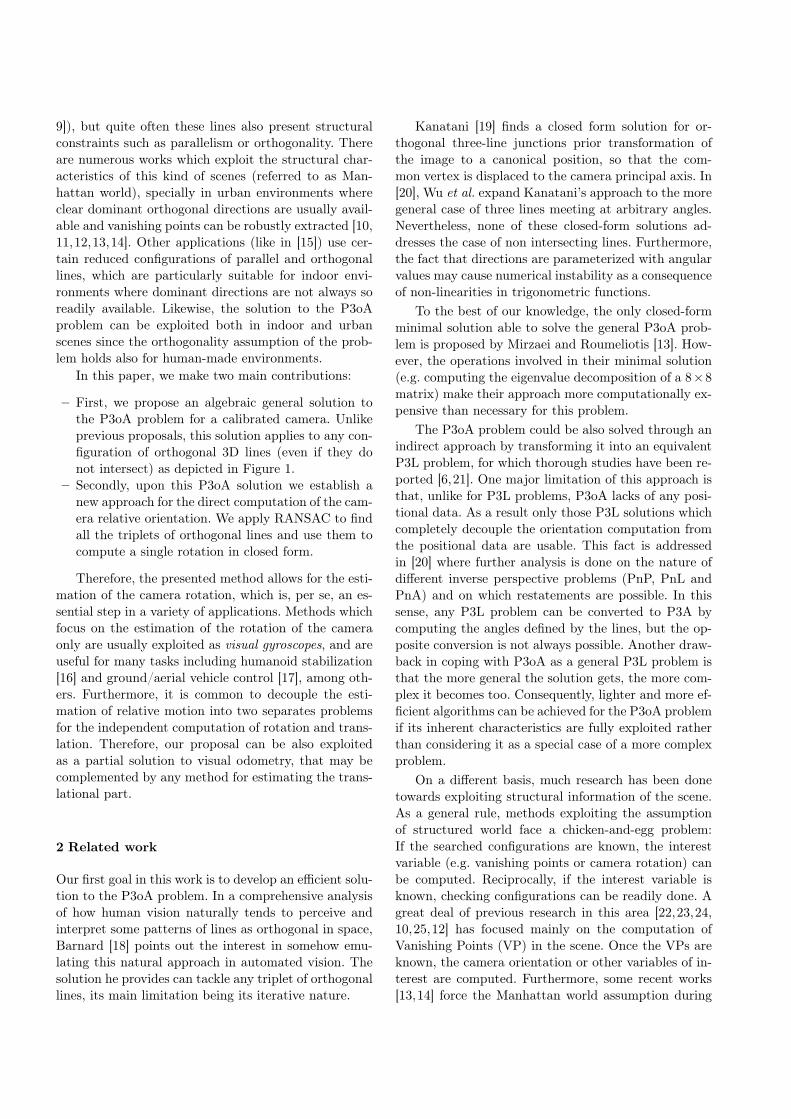
3.4 Revisiting the case of orthogonal meeting lines.
Firstly, we revisit the resolution of the special case inwhich all three image lines meet in a single point. Insuch cases the interpretation planes form a pencil ofthree planes (see Figure 3).
The pencil direction t is defined as the normalizeddirection of the pencil axis, which can be computedfrom the intersection of any two planes in the pencil
t =ni × nj
‖ni × nj‖(6)
A feasible basis for each interpretation plane Πk inthe pencil is
Ωk =[t t×nk
](7)
This special basis will be referred to as the pencil basisfor the intepretation plane Πk. It can be seen from thedefinition of t in (6) that t ⊥ nk, so ‖t× nk‖ = 1 andthe pencil basis is orthonormal.
Under the parameterization of pencil bases, the bi-linear forms in (5) becomes diagonal in an elegant andseamless way (see Appendix A):
Bij =
[1 0
0 −αij
](8)
with
αij = − (t× ni)>
(t× nj) = −n>i nj (9)
As a consequence, using pencil bases permits us to ex-press each bilinear form Bij through a single scalar
Fig. 3 P3oA problem for meeting lines: The intepretation planesform a pencil of planes. Both +ν1 and −ν1 represent the samedirection
value which equals, up to sign, the cosine of the anglebetween the interpretation planes Πi and Πj . The in-herent duality when computing the angle between twoplanes disappears when a fixed representation nk istaken for every plane normal.
Under the pencil parameterization the condition (4)can be written as
ρi,1 ρj,1 − αij ρi,2 ρj,2 = 0 (10)
with ρk,· the components of the vector ρk:
ρk =
[ρk,1ρk,2
]Assuming that the second component of any ρk vec-
tor is non zero (which is always true for non degeneratecases, as discussed in Section 3.4.2), let us define thenew unknowns
rk =ρk,1ρk,2
(11)
The problem in (10) can be rewritten then as a simplersystem of quadratic equations
r1r2 = α12
r2r3 = α23 (12)r3r1 = α31
and taking into account the product of the three equa-tions
(r1r2r3)2
= α12α23α31 ⇒ r1r2r3 = ±√α12α23α31
the unknowns can be cleared as
rk =α
αij

with α = ±√α12α23α31.Therefore, each vector ρk can be solved from the
calculated rk by applying the condition ‖ρk‖ = 1
ρk,1ρk,2
=α
αij
ρ2k,1 + ρ2k,2 = 1
and the reduced solution to the P3oA problem takes aclosed form expression
ρk = ± 1√α2 + α2
ij
[α
αij
](13)
Once the reduced vector ρk is known, the corresponding3D direction νk can be recovered from (3) as
νk =[t t×nk
]ρk.
Hence, the resolution for the case of intersectinglines reduces to the steps given in Algorithm 1.
Algorithm 1 P3oA solution for intersecting linesData:n1, n2, n3 . interpr. planes normalss . Necker’s sign
Require: det([n1 n2 n3)
]) = 0
1: function P3oA_meeting(n1, n2, n3, s)2: α12 ← −n>1 n2, α23 ← −n>2 n3, α31 ← −n>3 n1
3: α← s · √α12α23α31
4: for k ← 1, 3 do5: ρk ← 1√
α2+α2ij
[α, αij
]>. get reduced solution
6: Ωk ←[t t× nk
]. build k-th pencil basis
7: νk ← Ωk ρk . undo pencil parameterization8: end for9: end function
3.4.1 Analysis of multiple solutions
The expression (13) leads to a total of 16 solutions dueto 4 sign ambiguities. However, the 3 outer signs affect-ing each ρk vector are due to the inherent ambiguity inline direction since, given a point, the lines with direc-tions +νk and −νk represent exactly the same entity(see Figure 3).
Therefore, only the sign of the parameter α requiresour attention. This sign is linked to the existence of twodistinct sets of directions which are solution to the sameP3oA problem. This duality, which has been known fora long time, is named the Necker’s cube illusion and hasbeen already pointed out by other authors when solvingthe P3A problem [20]. This illusion is displayed in Fig-ure 4, where we can notice that exactly the same threesegments may be perceived as a concave or a convextrihedron of two different cubes.
(a) Natural perception (b) Unusual perception
Fig. 4 Necker’s cube illusion: For the same image two inter-pretations are possible for both meeting (blue) and non-meeting(green) cases
3.4.2 Analysis of degenerate cases
A P3oA problem is degenerate if two lines have thesame projection in the image. In such a case, the twointerpretation planes corresponding to the coincidentlines become the same, and the remaining interpreta-tion plane is orthogonal to the other two (see AppendixB for a complete proof). Note that the orthogonality be-tween interpretation planes does not involve that linesin the image are orthogonal to each other, since
n>i nj ∝ l>i (KK>)lj = 0 ; l>i lj = 0.
Fig. 5 Degenerate case: lX and lY are degenerate, so the rela-tion ni ‖ nj ⊥ nk stands. Note that the orthogonality conditionis between interpretation planes, not image lines. There exist in-finite other pairs of lines X′ and Y ′ contained in the plane XYwhich would produce the same image
Let us assume, without loss of generality, that thelines Li and Lj are the source of the degeneracy (seeFigure 5 above). Then, according to the results in Ap-pendix B, the interpretation planes’ normals fulfill
ni ‖ nj , nk ⊥ ni, nk ⊥ nj
and according to (9) the pencil basis parameters be-come
αij = 1
αjk = αki = 0
For this particular configuration, the system of quadraticequations (12) reads
rirj = 1
rjrk = 0
rkri = 0

from which it is easy to conclude that rk = 0. As aresult
rk = ρk,1/ρk,2 = 0
‖ρk‖2
= ρ2k,1 + ρ2k,2 = 1
⇒ ρk =
[0
1
]This allows us to fully recover the direction of Lk from(3) as
νk = t× nk.
The pencil direction t can be computed as
t =nk × ni
‖nk × ni‖,
and, since nk⊥ni, we have ‖nk × ni‖ = 1 and the finalresult is
νk = (nk × ni)× nk
= −(n>i nk)nk + (n>k nk)ni = ni.
However, the unknowns ri and rj cannot be computedwith the remaining data. Instead, only the constraintthat the corresponding directions νi and νj are orthog-onal is kept. As a result, the direction correspondingto the non-degenerate line Lk can be fully recovered,whereas those of the degenerate lines Li and Lj areonly constrained to be a pair of orthogonal directionsinside the degenerate interpretation plane:
νk = ni = nj
νi ⊥ νj ,[νi,νj
]= Null
(ν>k)∈ Πi = Πj
A second special degenerate configuration would hap-pen when the assumption ρk,2 6= 0, made when definingrk in (11), does not hold. This however would mean thatfor the line Lk the direction is
νk =[t t×nk
] [10
]= t (14)
but the pencil direction t and the line direction νk canonly be the same if the camera center lies in Lk and, insuch a case, the line projects into the image as a point.This case lacks interest for us since we expect lines tobe segments in the image, not points.
3.5 Extension to the case of non-meeting orthogonallines
The solution to the P3oA problem with three meetinglines can be taken as the starting point to solve theP3oA general case, that is, when the lines in image donot intersect at a single point.
Let us assume that the image projections lk of threegeneric orthogonal 3D lines L1, L2, L3 are given. Their
corresponding interpretation planes Π1, Π2, Π3 no longerintersect at a single line, so there exists no set of basesΩk for which three diagonal bilinear forms, as those of(8), arise simultaneously. It is possible to build, how-ever, an equivalent problem replacing Lk by an auxil-iary line L∗ with its same direction, whose image pro-jection intersects with those of Li and Lj at a singlepoint (see Figure 6). That is equivalent to impose thatthe interpretation planes form a pencil of planes, whichin terms of the plane normals is fulfilled when
det([ni nj n∗
]) = 0. (15)
From now on, this equivalent problem will be referred
Fig. 6 General P3oA problem: It is always possible to create aequivalent virtual problem with lines meeting at the same point.Here l∗ replaces l2
to as the virtual problem, and the auxiliary line L∗and all related variables will be also tagged as virtual,with the symbol ∗. The solution to the virtual problemwould be the one already presented for the special caseof meeting lines (13).
Although the image l∗ for the virtual line is notknown, by definition it must fulfill the meeting condi-tion in (15), so the corresponding normal n∗ can be ex-pressed as a linear combination of ni and nj , or equiv-alently, n∗ must be orthogonal to the pencil directiont, so it can be expressed as
n∗ = Ωt δ (16)
withΩt being an orthonormal basis for t> right nullspaceand δ a reduced representation for n∗, so that δ ∈ S1.
Using the parameterization given in (3)
νk = ν∗ = Ω∗ ρ∗

and substituting the expressions for the pencil basis (7)and the meeting-case solution (13), the direction for lineL∗ (and so for Lk) is
νk = ν∗ =±1√
α2 + α2ij
[t [t]×n∗
]3×2
[α
αij
]2×1
, (17)
where all the parameters are relative to the virtualproblem (so they depend on the unknown δ too). Sincewe do know the interpretation plane for the original Lk,the extra condition
n>k νk = 0
can be applied to solve δ. Replacing νk with (17) in thecondition above, the equation to solve reads
α · n>k t+ αij · n>k [t]×n∗ = 0 (18)
with
α = ±√α∗iαijαj∗ (19)
α∗i = −n>∗ ni, αij = −n>i nj , αj∗ = −n>j n∗
The two solutions of equation (18) are contained in theset of 4 solutions of an equivalent quadratic equation
n>∗ Qn∗ = 0 (20)
with
Q =1
2
(n>k t)2
αij
(nin
>j + njn
>i
)+ [t]×
(nkn
>k
)[t]×
(21)
as deducted in Appendix C.We substitute in the equivalent equation (20) the
parameterization given in (16) so that the final problemto solve becomes
δ>Qt δ = 0 (22)
defined by the equivalent quadratic
Qt = Ω>t QΩt (23)
The symmetric matrix above can be diagonalized, e.g.via SVD or eigendecomposition, into
Qt = U
[d1 0
0 d2
]U> (24)
with U a 2 × 2 orthonormal basis. From this decom-position it can be concluded that the solutions to (22)fulfilling δ ∈ S1 are
δ =1√
|d1|+ |d2|U
[+√|d2|
±√|d1|
](25)
as long as sign(d1) 6= sign(d2). As a result, it is a nec-essary condition that the 2 × 2 quadratic form Qt isnon-definite for a solution to the P3oA problem to ex-ist. The case in which Qt is semidefinite (non full-rank)corresponds to the previous case of meeting lines. Thus,from now on we consider the cases for which Qt is in-definite.
Once δ is solved, the seeked virtual normal n∗ canbe recovered from (16). Two possible n∗ are obtaineddue to the sign indeterminacy in (25), each correspond-ing to a mathematically feasible world model. Further-more, each of them outcomes two possible solutions be-cause of the duality in the P3oA problem. So, the num-ber of reachable solutions adds up to 4, from which 2are false solutions that appear when squaring the radi-cal equation. However, for a given n∗ solution, the value|α| is completely defined by (19) and the correct signfor α = s |α| can be extracted from the original radicalequation (18)
s = − sign(αij · n>k [t]× n∗
|α| · n>k t) (26)
Once both n∗ and the correct sign(α) are known foreach case, the simple solution depicted in Algorithm 1can be applied to solve each virtual problem, therebyobtaining two possible solutions to the original problem.
The general P3oA procedure described above is de-picted in Algorithm 2.
4 Application of the P3oA solution to visualodometry
In this section the P3oA problem is exploited to ob-tain a minimal solution for the camera relative rotationbased on the observation of a single triplet of orthog-onal lines in two different frames. We propose, then,a robust framework which employs all the orthogonalconfigurations available to estimate the camera relative(incremental) rotation. Therefore, the presented algo-rithm can be used as a visual gyroscope.
Furthermore, since the estimation of relative motionis often decoupled in estimation of rotation and transla-tion, our solution can be used to address visual odome-try if it is complemented by any method for estimatingthe translational part (e.g. the proposal in [15]).
4.1 Minimal solution for the relative rotation
Let νk3k=1 be a set of three orthogonal directions com-ing from the minimal solution of a P3oA problem (see

Algorithm 2 General P3oA algorithmData:K . camera intrisic calibrationl1, l2, l3 . homogeneous image lines
Result:ν1,ν2,ν3 . 3D directions in camera frame
Initialization:1: for k ← 1, 3 do2: nk ← NS(K>lk) . get interpr. plane normal3: end forGeneral P3oA resolution:4: if det(
[n1 n2 n3)
]) = 0 then . if intersecting lines
5: for m← 1, 2 do6: ν(m)
k 3k=1 ← P3oA_meet(n1,n2,n3, (−1)m)7: end for8: else . if non-intersecting lines9: take two normals (e.g. n1 and n2)10: t← NS(n1 × n2) . pencil direction11: Ωt ← Null
(t>)
. pencil nullspace12: build equivalent quadratic Qt . see (21) and (23)13: solve δ(m) from SVD(Qt) . see (25)14: for m← 1, 2 do15: n∗ ← Ωt δ
(m) . compute virtual normals16: compute s sign for n∗ . see (26)17: ν(m)
k 3k=1 ← P3oA_meet(n1,n2,n∗, s)18: end for19: end if
* NS(·) ≡ ·‖·‖ . Abbreviation for normalization
Section 3). We stack them as the columns of an or-thogonal direction matrix V ∈ O(3). As shown in Sec-tion 3.4.1, there are 16 valid solutions for a minimalP3oA problem: Due to Necker’s duality the solutionproduces two geometrically distinct sets of directionsV (m), where we use the upper index m=1, 2 to dis-tinguish both Necker alternatives. On the other hand,each direction is recovered up to sign. The sign ambi-guities can be gathered into a diagonal sign matrix, sothat the whole set of 16 solutions for a minimal P3oAproblem is represented by the single expression V (m)S,where
S =
s1 0 0
0 s2 0
0 0 s3
, si = ±1. (27)
Let Rrel and trel be the relative rotation and trans-lation, respectively, of the camera in the second framewith respect to (wrt) the camera coordinate system inthe first frame. The relative rotation between the framescan be solved from the directions of the triplet of or-thogonal lines observed in both frames. The 3D direc-tions coming from the solution of the P3oA problem ineach frame are
V(m1)1 S1, V
(m2)2 S2, (28)
so one could think that the combination of both wouldproduce 256 different solutions for Rrel. This is not
so, though. All the possible solutions for Rrel can becondensed into the expression
Rrel = V(m1)1 S1S
>2 V
(m2)2
>, (29)
and this simplified into
Rrel = V(m1)1 S V
(m2)2
>, (30)
where
S = S1S>2 =
s1,1s2,1 0 0
0 s1,2s2,2 0
0 0 s1,3s2,3
=
s1 0 0
0 s2 0
0 0 s3
.We also impose the constraint det(Rrel) = +1 to assurethat Rrel is a valid rotation:
det(Rrel) = det(V(m1)1 S V
(m2)2
>)
= det(V(m1)1 ) det(S) det(V
(m2)2 )
= s1s2s3 det(V(m1)1 ) det(V
(m2)2 ) = +1.
As a result, the condensed expression for all the possiblesolutions can be finally reduced to
Rrel = V(m1)1 S V
(m2)2
>(31)
s1, s2 = ±1, s3 = s1s2 det(V(m1)1 ) det(V
(m2)2 ).
The conclusion is that 4 degrees of freedom (2 for Neckerduality and 2 for direction signs) are retained and thereare 24 = 16 solutions for the relative rotation. However,when working with keyframes in a video sequence as invisual odometry [28], it makes sense to assume thatthe relative rotation between any two frames is wellbelow 90 degrees. We will show next how this smallrotation assumption allows us to further reduce the so-lution multiplicity to only two potential solutions. If itwere not the case that rotation angle was small, but bigchanges of view could occur, other approaches could beadopted such as examining the gradient at the segmentsto determine if they are flipped between the two images[15].
4.1.1 Sign ambiguity
Under the small rotation assumption, the sign matrixS in (31) is taken so that the rotation Rrel is closest toidentity, that is:
S = diag(sign(diag(V(m1)1
>I3V
(m2)2 ))).
As a result, the multiplicity coming from the signambiguities (two degrees of freedom) is removed andonly 4 solutions remain due to Necker’s duality.

4.1.2 Necker ambiguity
Let V i and V ∗i stand for the true and dual (false) so-lution, respectively, for a certain instance of the P3oAproblem due to Necker duality. From (31), the four pos-sible combinations of Necker modalities are
(V 1,V 2), (V ∗1,V 2), (V 1,V∗2), (V ∗1,V
∗2).
Under the small rotation assumption, half of the combi-nations can be ruled out through a simple heuristic rule:corresponding Necker configurations are closer than noncorresponding ones. Different metrics can be applied tomeasure this distance, e.g. the angular distance definedin equation (34).
Once this distinction is applied, only the two combi-nations (V 1,V 2), (V ∗1,V
∗2) remain. When more so-
lutions are available, the selection between these twooptions can be performed within the RANSAC step, asdescribed in the next section. However, if no parallaxexists between frames both pairs provide exactly thesame solution, as explained in Appendix D.
4.2 Robust estimation from multiple configurations
The robust estimation of the relative rotation using allthe triplets of orthogonal lines available in the scenecomprises a series of steps: Firstly, all possible tripletsof segment matches among the images are considered,and this set is reduced by pruning non feasible combina-tions. The remaining triplets are classified in a RANSACframework and finally a global estimation of the rota-tion is performed from all the inlier triplets.
4.2.1 Filtering feasible candidate triplets
In the proposed approach (Algorithm 3) it is first nec-essary to generate all possible 3-combinations from, say,N∗ segment matches among images, whose number addsup to(N∗
3
)=
N∗!
3!(N∗ − 3)!=
1
6N∗(N∗ − 1)(N∗ − 2),
so the number of candidates grows with the cube of N∗.However, many of these generated combinations are notfeasible candidates. Therefore, it is most interesting toprune the large list of candidates in advance, which canbe done by checking the solvability of the arising nu-merical problem. This simple test allows us to rule outmany of the generated candidate triplets, so that onlyN of the original N∗ remain.
Depending on the case to be solved, a different con-dition stands for a given configuration of normals to
be solvable. For meeting lines (Section 3.4), since thesolution depends on the parameter
α =√α12α23α31
it is clear that the product inside the square root shouldbe positive and the condition becomes
α12α23α31 > 0 (32)
As for non meeting lines (Section 3.5), the equivalentquadratic Qt must be indefinite, which in the 2×2 casereduces to
det(Qt) < 0 (33)
Each triplet of matches comprises two triplets of nor-mals, one per image, and the conditions above must befulfilled by both.
4.2.2 Finding true configurations
From now on, R will stand for the relative rotationbetween the two camera frames. The direction matri-ces for the k-th triplet of lines in the first and secondimage are, respectively, V (m)
1,k and V (m)2,k , and the corre-
sponding rotation candidate computed by the minimalsolution (in Section 4.1) is denoted as R(m)
k .From the pruned list of N triplets, 2N candidates
R(m)k are computed for the relative rotation R, many
of which may be outliers generated due to non orthog-onal combinations, false Necker configurations, wrongmatchings, bad segment detections, etc. Thus, RANSACis applied to find the relative rotation with maximumsupport among all the available candidates. The good-ness of this approach bases on the sensible assumptionthat triplets which are not orthogonal will vote for ran-dom rotations and will not support a concrete solution.Since only one sample is necessary for each RANSACstep, the number of iterations and the computationalcost is relatively low.
A metric is needed in the RANSAC framework tocheck if the hypothesis is fullfilled, for which the angulardistance for rotations [29] has been chosen
d(Ra,Rb) ≡ d∠(Ra,Rb) = θ
= 2 arcsin(‖Ra −Rb‖F
2√
2). (34)
Here ‖·‖F stands for the Frobenius norm defined as
‖A‖F =
√trace(A>A). (35)
The necessary threshold θ to decide if two rotationsstand for the same solution is set to θ ≈ 1.5, since thevariance of the solutions due to noise tends to be of thatorder.

Algorithm 3 Incremental rotation computationData:K . camera intrisic calibrationl1,k . lines in image #1l2,k . lines in image #2M . 2×N∗ matches matrix
Result:R . Rotation of the camera between frames
Compute rotation candidates:1: generate all triplets of matchesΓ N∗
k=1 ← nchoosek(M , 3)2: filter non-solvable triplets: . see Section 4.2.1Γ Nk=1 ← Γ
N∗k=1
3: for k ← 1, N do . for each triplet4: for i← 1, 2 do . for each image5: V i ← P3oA(l1, l2, l3) . see Algorithm 26: end for7: Rk ← V 1 S V
>2 . see Section 4.1
8: end forRANSAC filtering:9: find candidate with maximum support and inliers I:I ← argmax(#R : d(Rk,R) < θ, R ∈ Rk)
Global optimization:10: Υ1 ←
[V 1,I
], Υ2 ←
[V 2,I
]. stack 3D directions
11: URΣR V R = Υ1Υ>2 . compute SVD12: R = URV
>R . Procrustes resolution
4.2.3 Global refinement
To increase the precision of the method, the final es-timate of the camera rotation R is computed throughthe optimization of a cost function which involves allthe valid candidates obtained from the prior step.
Formally, we address the task as a least squares op-timization problem in which we minimize the sum ofthe squared distances between corresponding directionmatrices after transformation by R, that is
R = argminR
(∑
k∈inliers
dist2(V 1,k,RV 2,k)). (36)
When working with rotations, there are several com-mon alternatives to measure distances [29]. The angulardistance defined in (34) is usually considered the mostnatural metric for rotations in SO(3). However, we pre-fer here the chordal distance [29] defined as
dchord(Ra,Rb) = ‖Ra −Rb‖F (37)
because due to its quadratic nature it yields simplerexpressions than the angular distance. For the samereasons, this metric has been used before in [30]. In-terestingly, when the residuals are small (as one wouldexpect in the global optimum) both metrics are equiv-alent up to a first-order approximation [29,30]:
d2chord = 8 sin2(θ/2) ≈ 8(θ/2)2 = 2 d∠
2 (38)
The substitution of the chosen metric (37) into theleast squares problem (36) yields the optimization prob-lem
R = argminR
(∑
k∈inliers
‖V 1,k −RV 2,k‖2F) (39)
This is equivalent to the orthogonal Procrustes problem[31] defined as
R = argminR
(‖Υ1 −RΥ2‖2F), (40)
where Υ1 and Υ2 are the concatenation of the inlier di-rection matrices V 1,k and V 2,k, respectively. This prob-lem admits a closed-form solution [32] and the globalminimum is attained for R = URV
>R, where UR SRV
>R
is the Singular Value Decomposition of Υ1Υ>2 .
5 Experimental Results
In this section we evaluate and analyze the performanceof our two main contributions: A minimal solution tothe P3oA problem and a visual gyroscope based on theuse of this minimal solution. Thus, the experimentsare divided into two main groups. First we focus onthe comparison of the proposed minimal solution withother existing alternatives, and then we present an ex-tensive set of experiments in which its application toa visual gyroscope is tested and compared to state-of-the-art methods.
5.1 Minimal solutions
A minimal solution provides the exact solution (or mul-tiple mathematically feasible solutions) from a minimalset of input data. However, even though a minimal solu-tion took ideal data unaffected by noise, working underfinite precision arithmetic could still provoke numericalissues that can deteriorate the performance introducingsome degree of error.
For this reason, we use here ideal data to test ourproposed minimal solution and other related minimalalternatives using ideal, error-free data as input in or-der to extract meaningful conclusions on the numericalbehaviour and stability of the solutions.
As already shown in some previous work [13], thereare two distinct minimal configurations of lines in aManhattan world from which the Manhattan directionscan be recovered:
1. The three lines are orthogonal to each other (seeFigure 1(a) or Figure 7(a) in blue): This is the caseof the P3oA problem addressed in this work, alsoconsidered by Mirzaei and Roumeliotis in [13].

(a) Minimal cases: 3 orthogonallines (blue), 2 par. lines + 1 ort.line (orange)
1e-14 1e-13 1e-12 1e-11 1e-10 1e-09 1e-08 1e-07 1e-06 1e-05 1e-04
Rotation error (deg)
0
10
20
30
40
50
60
70
80
90
Occu
rre
nce
s (
%)
Ours
Mirzaei
Elqursh
(b) Histogram of numerical errors
Fig. 7 Numerical evaluation of minimal solutions. (a) Synthetic data: A P3oA minimal configuration (3 orthogonal lines, in blue)and a triplet formed by 2 parallel lines and 1 orthogonal line (orange) (b)(c) The histogram (for 106 samples) of the numerical errorsshows higher numerical stability for our approach compared to the solution of P3oa with the alternative solver [13] (green) or thesolution of the 2 par. + 1 ort. minimal problem with [15] (orange)
2. Two lines are parallel, and the third line is orthogo-nal to them (see Figure 7(a) in orange): This is thecase exploited by Elqursh and Elgammal in [15].
To obtain the necessary evaluation data we assumea ideal camera with a horizontal Field of View (FOV)of 50 and a 4:3 aspect ratio. We generated then 106
random triplets of lines (asserting they lie inside thecamera’s field of view) for both of the minimal problemsmentioned above. Since multiple solutions arise for theminimal cases only the one corresponding to the groundtruth is kept for evaluation.
In this section we are going to show:
– The differences betweenminimal solvers for the P3oAproblem. This minimal problem can be solved moreaccurately and faster using our proposed solutionthan with the alternative solution presented in [13].
– The differences between the two minimal problemsconnected to the Manhattan world, using our solverfor the P3oA problem and the simple minimal solu-tion in [15] for the 2 parallels + 1 orthogonal con-figuration.
5.1.1 Comparison of the P3oA solvers
For the same set of 106 random P3oA problems, wecompare the performance of our proposed minimal so-lution in Algorithm 2 to the minimal solution providedby Mirzaei and Roumeliotis [13].
The evaluation results depicted in Figure 7(b) showthat our minimal solution is more accurate and nu-merically stable than the Mirzaei-Roumeliotis’ alterna-tive, with a difference of several orders of magnitude inthe numerical error. Furthermore, our approach is alsomore computationally efficient: The average run timefor our Matlab implementation is 0.9 ms whereas the
mean time for Mirzaei-Roumeliotis’ is of 8.2 ms, thatis, almost an order of magnitude lower.
This could be expected for two main reasons. On theone hand, our solution directly addresses the particu-lar case of the P3oA problem, exploiting the intrinsiccharacteristics of the configuration. On the other hand,the minimal solution in [13] stems from the particular-ization of a closed-form solution to the estimation ofManhattan world directions from an arbitrary numberof observed lines. This is a more complex problem, andso is also its solver. As a result, the particularizationfor the minimal problem, although simpler, still keepspart of such complexity. This behaviour can be alsoexplained from a more practical point of view lookingat the operations involved: our minimal solution reliessolely on dot and vector products, and at some pointthe eigenvalue decomposition of a 2×2 matrix. Mirzaei-Roumeliotis’s method, however, needs to perform theeigenvalue decomposition of a 8×8 matrix, among otheroperations. Since the decomposition of the matrix be-comes worse conditioned for bigger matrices, this mayalso explain the observed numerical behaviour.
5.1.2 Comparison of the minimal problems
We assess the numerical behaviour of the solutions tothe minimal problem of orientation from lines in a Man-hattan world in its two possible forms. For that, wesolved 106 random minimal cases of orthogonal lineswith our approach (in Algorithm 2) and other 106 ran-dom cases of 2 parallel + 1 orthogonal lines with theminimal solution proposed by Elqursh and Elgammal[15].
We observe from the results in Figure 7(b) that,although Elqursh-Elgammal’s solution performs well,ours does better with a typical numerical error one or-der of magnitude lower.

The numerical complexity of Elqursh-Elgammal’sminimal solution is similar, or even lower, than our al-gorithm: Just linear operations, mainly dot and vec-tor products. Hence, we guess that the lower numericalstability of Elqursh-Elgammal’s solution stems from ahigher occurrence rate of near-degenerate cases in the2 parallels + orthogonal minimal problem than in the3 orthogonals case. This suggests, at least qualitatively,that the exploitation of the P3oA problem may providehigher robustness.
5.2 Visual gyroscope
The proposed approach for the estimation of relative ro-tation between frames (Algorithm 3) can be used as avisual gyroscope. A commonly used approach for a line-based visual gyroscope resorts on the extraction of theVanishing Points (VP) in each image and the compu-tation of a rotation from those VPs. An alternative tothese Vanishing Point-based (VP-based) methods arethe Minimal Solution-based (MS-based) methods, suchas ours or Elqursh-Elgammal’s in [15]. These do notrely on the computation of the scene VPs but on ex-ploiting the existence of any minimal Manhattan con-figuration. The pipelines of our proposal and that ofElqursh-Elgammal are very similar, being the main dif-ference the particular minimal solution upon which themethod is built. This is more in-depth analyzed next.
5.2.1 Comparison of the Minimal Solution-basedmethods
Here, we show a series of experiments aimed at assess-ing the performance of our method against the one re-ported by Elqursh and Elgammal in [15] under differentconditions and variables.
To make the analysis and conclusions clearer, wechoose a very simple testing scenario, consisting of ascene containing just one cube, which provides a con-trolled amount of lines in Manhattan directions only,so configurations for both algorithms are available.
In order to have perfect, reliable groundtruth of therotation we generate the described cube scenario syn-thetically. The metric chosen for error computation isagain the rotation angle defined in (34).
To generate the synthetic data we simulate a 1m×1m× 1m cube (see Figure 8(a)) and the camera is ran-domly placed at distances below 9 m. We assert thatthe entire cube is projected onto the image and that, foreach pair of images, the same lines are simultaneouslyobserved.
The simulated camera (with no distortion) is char-acterized by the calibration matrix
K =
700 0 320
0 700 240
0 0 1
(41)
which provides a horizontal field of view (FOV) of 49.The results, derived from a population of 104 sam-
ples, are depicted graphically by means of boxplot dia-grams: the central line is the median and the lower andupper borders of the box represent the 25th and 75thpercentiles, respectively.
Image noise resilience This error is due to camera noiseand image-related artifacts that affect the precision ofthe input line data. We simplify all the factors affectingthe data quality into a single random noise added tothe image coordinates of the segment end-points. Thenoise is modeled by a Gaussian distribution with zeromean and an increasing standard deviation σc.
The results depicted in Figure 8(b) exhibit a lineartrend between the order of noise in the image and theorder of the rotation error. For the whole range of noiselevels considered, our method proves to be more precise.
Manhattan assumption The set of lines in real struc-tured scenes are not exactly parallel or orthogonal, sothe Manhattan assumption is violated. Therefore, wealso test the influence of deviations from the Manhat-tan assumption in the scene model.
In this experiment images are noise-free, but an in-creasing level of Gaussian noise σ⊥ is applied to the 3Dpoints of the cube (before projection). The immediateeffect is that the orthogonality or parallelism among 3Dsegments is no longer fulfilled. Values for σ⊥ spanningfrom 1 mm up to 1 cm were used and it can be seenin Figure 8(c) that both methods still yield good re-sults. So it can be concluded that both methods standbounded deviations from the Manhattan assumptionalthough, once again, our approach produces slightlybetter results for all the considered noise range.
Perspective distortion effect One important character-istic of the minimal solution exploited by Elqursh andElgammal is that it internally depends on the computa-tion of a Vanishing Point from two lines. The precisionachievable when computing vanishing points stronglydepends on the distortion arising from the scene per-spective projection, which maps points lying at infin-ity (namely the vanishing points) to finite points. Theweaker the perspective effect gets the farther the van-ishing points lie, becoming more sensitive to image noise[27]. This simple effect is depicted in Figure 9(a) for our

(a) Setup
0.001 0.01 0.1 1
10−3
10−2
10−1
100
101
P3oA
Elqursh
Rota
tion e
rror
(deg)
(b) Image noise
0.001 0.002 0.003 0.004 0.005 0.006 0.007 0.008 0.009 0.01
10−2
10−1
100
P3oA
Elqursh
Rota
tion e
rror
(deg)
(c) Structure noise
Fig. 8 Synthetic experiments on the noise resilience of our approach and Elqursh-Elgammal’s [15]. (a) The setup for the test. Thecube is observed from two poses and the relative transformation is solved. (b)(c) Our method outperforms Elqursh-Elgammal’s for allnoise levels (104 samples)
(a)
0.01 0.1 0.5
10
Rota
tion e
rror
(deg)
f (m)
(b)
Fig. 9 The perspective distortion effect greatly depends on theFOV of the camera. (a) Perspective distortion in large FOV (left)and reduced FOV (right) camera. (b) Our approach is noticeablymore robust that Elqursh-Elgammal’s [15] under weak perspec-tive
testing environment. On the other hand, the solution tothe P3oA problem used in our approach does not relyon vanishing points at all.
As a result the performance of both approaches shouldvary with the degree of perspective distortion intro-duced by the projective camera. In order to assess thiseffect we deploy an experiment in which focal distanceand camera zoom vary accordingly to modify perspec-tive deformation of the observed cube while keepingthe object size in the image constant. Figure 9(b) showshow as the perspective deformation becomes weaker forincreasing focal length the results provided by Elqursh-Elgammal’s algorithm get worse while ours even im-prove. However, for very small focal distances corre-sponding to wide FOV cameras Elqursh’s approach canbe slightly more precise than ours. This hints that itcould be fruitful to address a simultaneous exploita-tion of both approaches in order to get a more robustmethod for any kind of situation.
Verification of conclusions with real data Finally, tocontrast the results and conclusions obtained from thesynthetic experiments, we tested the same methods inthe cabinet dataset of the TUM Benchmark [33]. Thescene used for this dataset is very similar to that of
our previous synthetic framework. Namely, the datasetconsists of a continous video sequence of a plain cab-inet which is recorded with a Kinect device from dif-ferent viewpoints. The absolute pose groundtruth ofthe Kinect device for each frame is provided with thedataset, so that we can still evaluate the rotation errorquantitatively.
The borders of the cabinet have been detected andmatched for all the images of the sequence. Some ofthe pairs used in this experiment are shown in Figures10(a) and 10(b). We use superposition with false colorto visualize the pair of images simultaneously.
The statistics of the committed error, plotted in Fig-ures 10(c) and 10(d) and detailed in Table 1, confirmthe conclusion also reached from the synthetic results:Our algorithm tends to perform better than Elqursh-Elgammal’s, with higher precision and robustness.
Table 1 Statistics of error in the cabinet dataset [33]
Algorithm R estimation error (deg)Mean q1 Median q3
Ours 0.655 0.466 0.623 0.846Elqursh [15] 0.789 0.503 0.715 0.960
5.2.2 Real data evaluation
Finally, we analyze the performance of the Minimal So-lution-based (MS-based) algorithms and a more tra-ditional Vanishing Point-based (VP-based) algorithmbuilt upon the solution provided by Mirzaei and Roume-liotis in [13].
The methods are evaluated with the ICL-NUIM datasets[34], which provide video sequences recorded in a typicalstructured office environment. Lines were automaticallydetected using the LSD detector [35] and the match-ing between frames was performed using the LBD de-scriptor [36]. Then, the relative rotation was computed

(a) (b)
0
0.5
1
1.5
2
2.5
P3oA Elqursh
Rota
tion e
rror (d
eg)
(c)
0 0.5 1 1.5 2 2.50
10
20
30
40
50
60
70
P3oA
Elqursh
Rotation error (deg)
Occu
rrences (
#)
(d)
Fig. 10 Evaluation on real data. (a)(b) Two of the evaluatedpairs of frames (one example of available intersecting and nonintersecting orthogonal triplets marked in blue) (c)(d) Boxplotand histogram of the rotation error
between consecutive frames of the sequences and com-pared to the accompanying groundtruth. We calculatetwo different error metrics from each sequence:
– The root-mean-square error (RMSE), which due toits quadratic nature gives a good measure of therobustness. That is, if any of the committed errorsbecomes notably high, the RMSE grows accordingly.
– The median of the error, which is a good statisticfor the general precision of the method. Since themedian is much less affected by outliers, it capturesthe main trend of the error better than the RMSE.
The results in Tables 2(a) and 2(b) show that ourproposal outperforms the compared methods, achievinghigher precision and robustness than Elqursh-Elgammal’s[15], which agrees with the conclusions reached in all theprevious experiments.
As for the VP-based methods, they are expectedto perform well if the lines supporting the three or-thogonal vanishing points linked to a Manhattan worldframework can be clearly clustered (see Figure 11(a)).This explains why, in some cases, the median of theerror is lower for Mirzaei-Roumeliotis’s method (seeTable 2(b)). However, when there is no set of Man-hattan directions with a clear set of lines supportingit, the performance of this approach deteriorates andthe classification of the lines into Manhattan directionstends to fail (see Figures 11(b) and 11(c)). This caseis likely to happen when the number of lines lowers,when there are many more lines outside the Manhattanframework than inside, or the environment, although
structured, is not well modeled by the Manhattan as-sumption (see Atlanta world [37] or the mixture of Man-hattan frames [38]). This trait of the VP-based meth-ods makes them more prone to fail catastrophically,driving them to higher estimation errors. This justifiesthe significantly high RMSE in Table 2(a) obtained forMirzaei-Roumeliotis’ approach in the tested sequences.
Table 2 Metrics of the estimation error in ICL-NUIM datasets[34]
(a) RMSE of the rotation error
of kt0 of kt1 of kt2 of kt3Ours 0.557 0.447 1.151 0.416Elqursh-Elgammal [15] 0.585 0.719 1.505 0.420Mirzaei-Roumeliotis [13] 2.740 5.959 4.598 3.549
(b) Median of the rotation error
of kt0 of kt1 of kt2 of kt3Ours 0.317 0.231 0.459 0.232Elqursh-Elgammal [15] 0.365 0.292 1.071 0.232Mirzaei-Roumeliotis [13] 0.320 0.323 0.416 0.357
6 Conclusions
In this paper it has been presented a new closed-formsolution for the Perspective-3-Angles (P3A) problem inthe particular case that all angles are orthogonal (P3oAproblem). This solution can solve any configuration of3D orthogonal directions, both intersecting and non-intersecting lines. A purelly algebraic approach is de-rived to solve the most simple situation of meeting linesand then the solution is expanded to solve the most gen-eral case of non-meeting lines. The resulting solution isboth efficient and numerically stable, as validated ex-perimentally.
Secondly, a minimal solution has been presented forthe estimation of the relative rotation between two cam-eras based on the solution to the P3oA problem. Thisminimal solution has proven exploitable in a RANSACframework to classify triplets of lines fulfilling the or-thogonality constraint and a robust global solution us-ing all available triplets has been also proposed. Theperformance of this approach has been evaluated withboth synthetic and real data.

(a) Rich: VP Success (b) Poor: VP Success (c) Poor: VP Fail
Fig. 11 Examples of rich and poor Manhattan scenarios in the sequences of [34]. (a) The VP-based methods perform well in clearlystructured environments where the Manhattan directions are well supported. (b)(c) However, they easily fail when there is no clearsupport for the Manhattan directions.
A Reduction of pencil basis parameter
The bilinear map Bij is greatly simplified when pencil bases areused. The substitution of Ωk defined in (7) into (5) gives
Bij =[t t×ni
]>2×3
[t t×nj
]3×2
=
[t>t t>(t×nj)
(t×ni)>t (t×ni)>(t×nj)
]=
[1 00 −αij
]since ‖t‖ = 1 ⇒ t>t = 1 and by definition of the cross productt> (t× n) = 0 for any vector n.
The remaining parameter
αij = − (t× ni)> (t× nj)
can be further simplified to a single scalar product by applyingsome properties of the cross product. Firstly, the skew matrixrepresentation for the cross product as well as the property [t]>× =− [t]× allows us to write
αij = n>i [t]× [t]× nj
and then rewriting the product of skew matrices in the equivalentform
[a]× [b]× = ba> − (a · b)I3
the expression finally reduces to
αij = n>i(tt> − (t>t) · I3
)nj = −n>i nj
where it is used that t ⊥ nk by the definition in (6).
B Relations between interpretation planes forthe degenerate P3oA problem
Given a trihedron formed by three intersecting orthogonal lines, ifthe projection of two lines li and lj become the same, the normalsof the interpretation planes of the lines fulfill ni ‖ nj ⊥ nk.
The corresponding proof is developed in a sequence of minorsteps:– If the lines li and lj are parallel, so are the corresponding
normals ni and nj : li ‖ lj ⇒ ni ‖ nj .– If the normals ni and nj are parallel, the camera center must
lie in the IJ plane defined by the lines Li and Lj .– If the camera center lies in the IJ plane, the normal nk is
orthogonal to ni = nj .
B.1 Parallelism of ni and nj
Let li and lj be the homogeneous vectors corresponding to theprojection of the lines into the camera image. Since the projectiveentities li, lj ∈ P2 are defined up to scale, we use the similarityoperator li ∼ lj to represent the equality of both variables in theprojective space P2. Two vectors are then equivalent if they areparallel, or stated otherwise,
li × lj = 0.
The homogeneous lines in the image are related to the normalof the corresponding interpretation plane through the intrinsiccalibration matrix K [27]
n ∼K>l,
so the equivalency relation is transmitted to the normals:
ni × nj = (K>li)× (K>lj)
= det(K)K−>(li × lj) = 0⇒ ni ∼ nj
B.2 Position of the camera to fulfill ni ‖ nj
Let us assume, without loss of generality, that the three inter-secting lines fit the axes of the canonical coordinate system. As aresult, the direction of the lines in this particular case are givenby the canonical vectors ek3k=1. Denote the position and ori-entation of the camera as seen from this coordinate system ast and R, respectively. The normal to the intepretation plane ofeach line Lk, as seen from the camera, is then equal (up to scale)to
nk ∼ R>(ek × t). (42)
From the equivalency of the lines i and j it follows then that
ni ∼ nj ⇒ (R>(ei × t))× (R>(ej × t))
= R> ((ei × t)× (ej × t))= 0⇒ (ei × t)× (ej × t) = 0
and this expression is symbolically equivalent to
(ei × t)× (ej × t) = [ei × t]× [ej ]× t
= (te>i − eit>) [ej ]× t
= (e>k t) t

So, it is concluded that the equivalency ni ∼ nj is only possibleif t = 0 or e>k t = 0. The first solution forces the camera to bein the point of intersection of the three lines, but this makes nosense. The second solution implies that, for Li and Lj to projectinto the same image line li ∼ lj , the camera center must lie inthe plane defined by lines Li and Lj .
B.3 Orthogonality of normals when the camera lies inthe IJ plane
Now, we will prove that if the camera center lies in the IJ plane,the normal of the interpretation plane for the remaining line Lkis orthogonal to both ni ∼ nj . Say nk and ni are orthogonal,which is equivalent to state n>k ni = 0. Using the relation in (42)
n>k ni = (ek × t)RR>(ei × t)
= t> [ek]>× [ei]× t
= −t>(eie>k − (e>k ei)I3)t
= −(t>ei)(e>k t)
= −(e>i t)(e>k t) = 0
and the condition above is then fulfilled only if the camera centerlies in the JK plane, the IJ plane, or both. Similarly, if nk andnj are orthogonal (necessary from ni ∼ nj) the camera centerlies in the IJ plane, the IK plane, or both. As a result, we see thatif the camera lies in the IJ plane as assumed, the orthogonalityconstraints are fulfilled.
In conclusion we see that if the projection of two lines, li andlj , are coincident then the camera center lies in the plane formedby Li and Lj . This, at the same time, provokes that nk ⊥ ni, orequivalently, nk ⊥ nj .
C Reparameterization of radical equation as aquadratic form
The equation
n>k t · α+ αij · n>k [t]× n∗ = 0
defined in (18) is non-linear wrt n∗ due to the square root oper-ation in
α = ±√α∗iαijαj∗
= ±√− (n>∗ ni)
(n>i nj
) (n>j n∗
)which makes the equation radical. As usual for these equations,we separate both terms in the sum and square them to get analmost-equivalent quadratic equation(n>k t
)2 · (±√α∗iαijαj∗)2 = α2ij · (n>k [t]× n∗)
2(n>k t
)2αij
· α∗iαj∗ = (n>k [t]× n∗)2
Then, we substitute α∗i and αj∗ and arrange the matrix opera-tions
(n>k t)2
αij· n>∗
(nin
>j
)n∗ = (n>k [t]× n∗)
>n>k [t]× n∗
= n>∗ [t]>×(nkn
>k
)[t]× n∗
so that the condition above can be encoded by a quadratic form
n>∗
((n>k t)
2
αij· nin>j − [t]>× nkn
>k [t]×
)n∗ = 0
From all infinite matrix representations available for the quadraticform given above we choose the symmetric one
Q =1
2
(n>k t)2
αij
(nin
>j + njn
>i
)+ [t]×
(nkn
>k
)[t]×
which permits us to readily diagonalize the quadratic form byeigenvalue decomposition in a unique way.
Then, the original problem in (18) is equivalent to solving
n>∗ Qn∗ = 0
for the defined Q.
D Necker duality and parallax effect
The two distinct solutions of the P3oA problem for the case ofmeeting lines are mirrored wrt the plane whose normal is theback-projection direction t through the intersection point. Thisrelation can be easily expressed through a reflection or House-holder matrix [27]. Let V be the real solution and V ∗ the mir-rored one. The following relation stands:
V = Ht V∗ (43)
with Ht = I3 − 2 t t>/t>t. This relation only stands when thethree lines meet in a single point, otherwise there exists no re-flection fulfilling the relation (43), even though this duality stillexists (see green configuration in Figure 4).
Without loss of generality, we will use the case of meetinglines to prove that both dual solutions provide the same rotationin the case of zero baseline (pure rotation). In such cases, takingthe pair of false configurations will produce the relative rotation
R∗ = V ∗1 (V ∗2)>
= Hp1V 1 V>2 H
>p2
= Hp1 RH>p2
(44)
where pi stands for the 3D coordinates of intersection point ini-th image wrt the camera frame. A rigid transformation existsbetween p1 and p2
p1 = R p2 + trel
so that, in the case of zero baseline we have
Hp1 = I− 2Rp2p>2 R
>
p>2 p2= RHp2R
>
and substituting in expression (44) reveals that
R∗ = RHp2R>RH>p2
= R
As a conclusion, in the case of pure rotation the true andfalse solutions are the same. So, the greater the parallax effectdue to non zero baseline ‖trel‖, the bigger the difference betweenboth possible solutions.
Acknowledgements We would like to thank to Ali Elqursh forproviding us the source code of the odometry method of Elqurshand Elgammal [15].
This work has been supported by two projects: "GiraffPlus",funded by EU under contract FP7-ICT-#288173, and "TAROTH:New developments toward a robot at home", funded by the Span-ish Government and the "European Regional Development FundERDF" under contract DPI2011-25483.

References
1. B. M. Haralick, C.-N. Lee, K. Ottenberg, and M. Nölle, “Re-view and analysis of solutions of the three point perspectivepose estimation problem,” International Journal of Com-puter Vision, vol. 13, no. 3, pp. 331–356, 1994.
2. V. Lepetit, F. Moreno-Noguer, and P. Fua, “EPnP: An Accu-rate O(n) Solution to the PnP Problem,” International Jour-nal of Computer Vision, vol. 81, pp. 155–166, July 2008.
3. J. A. Hesch and S. I. Roumeliotis, “A direct least-squares(DLS) method for PnP,” in IEEE International Confer-ence on Computer Vision (ICCV), 2011, pp. 383–390, IEEE,2011.
4. S. Li, C. Xu, and M. Xie, “A robust O(n) solution tothe perspective-n-point problem,” IEEE Transactions onPattern Analysis and Machine Intelligence, vol. 34, no. 7,pp. 1444–1450, 2012.
5. F. M. Mirzaei and S. I. Roumeliotis, “Globally optimalpose estimation from line correspondences,” in IEEE Inter-national Conference on Robotics and Automation (ICRA),2011, pp. 5581–5588, Ieee, May 2011.
6. L. Zhang, C. Xu, K.-M. Lee, and R. Koch, “Robust and ef-ficient pose estimation from line correspondences,” in AsianConference on Computer Vision (ACCV), 2012, pp. 217–230, Springer, 2013.
7. S. Ramalingam, S. Bouaziz, and P. Sturm, “Pose estimationusing both points and lines for geo-localization,” in Roboticsand Automation (ICRA), 2011 IEEE International Confer-ence on, pp. 4716–4723, IEEE, 2011.
8. R. I. Hartley, “Lines and points in three views and the trifocaltensor,” International Journal of Computer Vision, vol. 22,no. 2, pp. 125–140, 1997.
9. A. Bartoli and P. Sturm, “Structure-from-motion usinglines: Representation, triangulation, and bundle adjustment,”Computer Vision and Image Understanding, vol. 100, no. 3,pp. 416–441, 2005.
10. J. Košecká and W. Zhang, “Extraction, matching, and poserecovery based on dominant rectangular structures,” Com-puter Vision and Image Understanding, vol. 100, no. 3,pp. 274–293, 2005.
11. G. Schindler, P. Krishnamurthy, and F. Dellaert, “Line-basedstructure from motion for urban environments,” in Third In-ternational Symposium on 3D Data Processing, Visualiza-tion, and Transmission, pp. 846–853, IEEE, 2006.
12. W. Förstner, “Optimal vanishing point detection and rota-tion estimation of single images from a legoland scene,” in IS-PRS Commission III Symposium of Photogrammetric Com-puter Vision and Image Analysis, pp. 157–162, 2010.
13. F. M. Mirzaei and S. I. Roumeliotis, “Optimal estimationof vanishing points in a Manhattan world,” in IEEE In-ternational Conference on Computer Vision (ICCV), 2011,pp. 2454–2461, IEEE, 2011.
14. J. C. Bazin, Y. Seo, C. Demonceaux, P. Vasseur, K. Ikeuchi,I. Kweon, and M. Pollefeys, “Globally optimal line cluster-ing and vanishing point estimation in Manhattan world,” inComputer Vision and Pattern Recognition (CVPR), 2012IEEE Conference on, pp. 638–645, IEEE, 2012.
15. A. Elqursh and A. Elgammal, “Line-based relative pose esti-mation,” in IEEE Conference on Computer Vision and Pat-tern Recognition (CVPR), 2011, pp. 3049–3056, IEEE, 2011.
16. M. Finotto and E. Menegatti, “Humanoid gait stabilizationbased on omnidirectional visual gyroscope,” in Workshop onHumanoid Soccer Robots (Humanoids’ 09), 2009.
17. E. Rondon, L. R. G. Carrillo, and I. Fantoni, “Vision-basedaltitude, position and speed regulation of a quadrotor rotor-craft,” in IEEE/RSJ International Conference on IntelligentRobots and Systems (IROS), 2010, pp. 628–633, 2010.
18. S. T. Barnard, “Choosing a basis for perceptual space,” Com-puter vision, graphics, and image processing, vol. 29, no. 1,pp. 87–99, 1985.
19. K. I. Kanatani, “Constraints on length and angle,” Com-puter Vision, Graphics, and Image Processing, vol. 41, no. 1,pp. 28–42, 1988.
20. Y. Wu, S. S. Iyengar, R. Jain, and S. Bose, “A new general-ized computational framework for finding object orientationusing perspective trihedral angle constraint,” IEEE Transac-tions on Pattern Analysis and Machine Intelligence, vol. 16,no. 10, pp. 961–975, 1994.
21. M. Dhome, M. Richetin, J.-T. Lapreste, and G. Rives, “De-termination of the attitude of 3d objects from a single per-spective view,” IEEE Transactions on Pattern Analysis andMachine Intelligence, vol. 11, no. 12, pp. 1265–1278, 1989.
22. A. Criminisi, I. Reid, and A. Zisserman, “Single view metrol-ogy,” International Journal of Computer Vision, vol. 40,no. 2, pp. 123–148, 2000.
23. M. E. Antone and S. Teller, “Automatic recovery of relativecamera rotations for urban scenes,” in IEEE Conference onComputer Vision and Pattern Recognition (CVPR), 2000.,vol. 2, pp. 282–289, IEEE, 2000.
24. J. Košecká and W. Zhang, “Video compass,” in EuropeanConference on Computer Vision (ECCV), 2002, pp. 476–490, Springer, 2002.
25. P. Denis, J. Elder, and F. Estrada, Efficient edge-basedmethods for estimating manhattan frames in urban imagery.Springer, 2008.
26. J. C. Bazin and M. Pollefeys, “3-line RANSAC for orthogo-nal vanishing point detection,” in IEEE/RSJ InternationalConference on Intelligent Robots and Systems (IROS), 2012,pp. 4282–4287, IEEE, 2012.
27. R. Hartley and A. Zisserman, Multiple View Geometry inComputer Vision. New York, NY, USA: Cambridge Univer-sity Press, 2 ed., 2003.
28. D. Nistér, O. Naroditsky, and J. Bergen, “Visual odometryfor ground vehicle applications,” Journal of Field Robotics,vol. 23, no. 1, pp. 3–20, 2006.
29. R. Hartley, J. Trumpf, Y. Dai, and H. Li, “Rotation aver-aging,” International Journal of Computer Vision, vol. 103,no. 3, pp. 267–305, 2013.
30. L. Carlone and F. Dellaert, “Duality-based verification tech-niques for 2D SLAM,” in Intl. Conf. on Robotics and Au-tomation (ICRA), 2015.
31. J. C. Gower and G. B. Dijksterhuis, Procrustes problems,vol. 3. Oxford University Press Oxford, 2004.
32. K. S. Arun, T. S. Huang, and S. D. Blostein, “Least-squaresfitting of two 3-d point sets,” Pattern Analysis and MachineIntelligence, IEEE Transactions on, no. 5, pp. 698–700, 1987.
33. J. Sturm, N. Engelhard, F. Endres, W. Burgard, and D. Cre-mers, “A benchmark for the evaluation of RGB-D SLAM sys-tems,” in IEEE/RSJ International Conference on IntelligentRobots and Systems (IROS), 2012, pp. 573–580, IEEE, 2012.
34. A. Handa, T. Whelan, J. McDonald, and A. Davison, “Abenchmark for RGB-D visual odometry, 3D reconstructionand SLAM,” in IEEE Intl. Conf. on Robotics and Automa-tion, ICRA, (Hong Kong, China), May 2014.
35. R. Grompone von Gioi, J. Jakubowicz, J.-M. Morel, andG. Randall, “LSD: a Line Segment Detector,” Image Pro-cessing On Line, vol. 2, pp. 35–55, Mar. 2012.
36. L. Zhang and R. Koch, “An efficient and robust line segmentmatching approach based on lbd descriptor and pairwise ge-ometric consistency,” Journal of Visual Communication andImage Representation, vol. 24, no. 7, pp. 794–805, 2013.
37. G. Schindler and F. Dellaert, “Atlanta world: an expecta-tion maximization framework for simultaneous low-level edge

grouping and camera calibration in complex man-made envi-ronments,” Proceedings of the 2004 IEEE Computer SocietyConference on Computer Vision and Pattern Recognition,vol. 1, pp. 203–209, 2004.
38. J. Straub, G. Rosman, O. Freifeld, J. J. Leonard, and J. W.Fisher, “A mixture of manhattan frames: Beyond the man-hattan world,” in Computer Vision and Pattern Recognition(CVPR), 2014 IEEE Conference on, pp. 3770–3777, IEEE,2014.