a methodology for using background pahs to support remediation decisions
TRANSCRIPT

A METHODOLOGY FOR USING BACKGROUND PAHs
TO SUPPORT REMEDIATION DECISIONS
Prepared for:
Southern California Gas Company and
Southern California Edison
Prepared by:
ENVIRON Corporation Emeryville, California
January 24, 2002 03-4150I

Y:\SCGC\White Paper\final paper\SoCal BG PAH method 122101.doc - ii - E N V I R O N
TABLE OF CONTENTS 1.0 Introduction.....................................................................................................................1-1
2.0 Development and Characterization of the Background PAH Data Base for Southern
California Surface Soil....................................................................................................2-1 2.1 Background Data Base for PAHs in Southern California Surface Soil .................2-1 2.2 Characterization of the Background PAH Data Base ............................................2-4
2.2.1 Evaluation of Homogeneity ........................................................................2-4 2.2.2 Consistency with a Common Distribution ..................................................2-6 2.2.3 Calculation of Summary Statistics..............................................................2-7 2.2.4 Summary of the Characteristics of the Background Data Set......................2-8
3.0 Use of the Background PAH Data Base to Support Site Investigation and
Remediation Decisions....................................................................................................3-1 3.1 Developing Site Investigation and Confirmation Sampling Plans .........................3-1 3.2 Characterizing Remediation Needs.......................................................................3-3
3.2.1 Common Approaches to Evaluating Background Data ..............................3-4 3.2.1.1 Point Estimates .........................................................................................3-4 3.2.1.2 Distributional Comparisons ......................................................................3-5
3.2.2 Practical Applications................................................................................3-7 3.2.2.1 An Initial Target Remediation Concentration............................................3-7 3.2.2.2 Delineating Lateral and Vertical Extent of PAHs Above Background Levels 3-83.2.2.3 Determining if PAH Levels Warrant Remediation....................................3-9
3.3 Evaluating Attainment of the Remedial Action Goals.........................................3-10 3.3.1 Graphical and Statistical Data Comparisons............................................3-10 3.3.2 Method for Calculating Volume-Weighted Average Concentration for PAH in Soil .................................................................................................................3-11 3.3.3 Evaluating Noncarcinogenic Effects of Total PAHs.................................3-12 3.3.4 Evaluating Ecological Effects of Total PAHs ..........................................3-13
4.0 References.......................................................................................................................4-1

Y:\SCGC\White Paper\final paper\SoCal BG PAH method 122101.doc - ii - E N V I R O N
LIST OF TABLES
Table 1: Southern California Former MGP Sites and Number of Background Samples From
Each Site Used in Background Data Set Table 2: Classification of PAHs by Category Table 3: Potency Equivalency Factors Table 4: Background Concentrations of Carcinogenic PAHs at Former MGP Sites, Total
B(a)P Equivalents Table 5: Smoothed Results Assigned to Censored Values Associated with Background Data
Set Table 6: Point Estimates of PAH Background Concentration in Soil Derived from Smoothed
Background Data Set
LIST OF FIGURES Figure 1: Location of Southern California MGP Sites from which Background Samples Were
Collected Figure 2: Quantile Plot of Southern California Background Data, Normal Distribution
Assumption (Unsmoothed Data Set) Figure 3: Quantile Plot of Southern California Background Data, Lognormal Distribution
Assumption (Unsmoothed Data Set) Figure 4: Quantile Plot of Southern California Background Data, Lognormal Distribution
Assumption (Smoothed Data Set)

Y:\SCGC\White Paper\final paper\SoCal BG PAH method 122101.doc 1-1 E N V I R O N
1.0 Introduction
The primary chemical constituents associated with residues from former Manufactured Gas Plant (MGP) sites are polycyclic aromatic hydrocarbons (PAHs). Although PAHs are indisputably one of the principal by-products of MGP operations, there are also many natural and anthropogenic sources of PAHs in the environment. Most notably, combustion of fossil fuels, structural fires, and various industrial activities form PAHs, as do such processes as wild fires and volcanic activities. As a result of these many sources, PAHs are found in virtually all surface soils in both urban and rural areas.
Using standard exposure assumptions and risk assessment methodologies for a residential exposure scenario, the concentration of carcinogenic Polycyclic Aromatic Hydrocarbons (CPAHs) in soil corresponding to a lifetime incremental cancer risk of one in a million, or even ten in a million, is less than the average background concentrations of CPAHs in California soils. (See Attachment A for a discussion of the CPAH concentration corresponding to a lifetime incremental cancer risk of one in a million.) As noted in agency guidelines, the Cal/EPA and USEPA (USEPA 1989b) do not require responsible parties to clean sites to levels lower than background. When facing the need to remediate a site for unrestricted land use at sites where background levels are above risk-based action levels, the most common risk management approach is to remediate to background levels. Characterizing background levels, however, is not necessarily easy; and determining a specific measure of background to use as the remediation target is even more difficult.
An important point to keep in mind, however, when making risk management decisions for former MGP sites is that remediation to background conditions is not the only management option available to project managers. It may not be the appropriate remediation goal for all sites. If, for example, a site is to remain in industrial service, risk-based remediation goals based on an industrial exposure scenario for workers may be well above background concentrations. Because lampblack and coal tar often leave a visible staining of soil, which may have a dark, streaked, or mottled appearance, project managers may elect to incorporate consideration of aesthetic factors into remediation decisions at former MGP sites. At some sites, for example, the project manager may consider it appropriate to remove any stained soil or visible lampblack, regardless of how the measured PAH concentrations compare against risk-based concentration goals or background levels. Depending in particular on the use of the site after its service as an MGP operation, chemicals other than PAHs may also be present in soil. Thus, the project manager may also need to assure that chemicals other than PAHs pose no health risk and that any cumulative health risks posed by PAHs in addition to other chemicals present are insignificant.
To address the often-encountered need to remediate CPAHs to background levels, we have developed a decision methodology for determining whether the CPAH concentrations at a particular Site differ from background concentrations. The methodology is designed to support the various site-management questions that typically arise during the investigation and remediation of an MGP site when remediation of CPAHs to background levels is an objective. Such questions include whether the unremediated site has CPAH levels above background levels. If so, additional questions are likely to include whether the lateral and vertical extent of contamination has been defined, what areas of the Site should be targeted for remediation, whether a proposed remediation

Y:\SCGC\White Paper\final paper\SoCal BG PAH method 122101.doc 1-2 E N V I R O N
will restore the site to background CPAH levels, and whether an implemented remediation has restored a site to background levels. In addition, because most former MGP sites have been put to some other use, buildings or other structures built after the MGP operations ceased are often present on former MGP sites. Accordingly, the safety and necessity of remediating under existing structures is often another question that the project manager faces.
The decision methodology we have outlined is designed to provide the project manager with a basis for determining whether the CPAHs present in soil at a site pose risks above those posed by background CPAHs. The decision methodology explicitly addresses the fact that cleaning to background levels is only one of several remedial objectives that a project manager may select. The decision methodology also provides the project manager with a decision framework to support selection of the optimal remedy for any particular site.
Because the background evaluation only addresses carcinogenic PAHs, it is necessary to supplement the background-based evaluation of CPAHs with a risk-based evaluation of the noncarcinogenic effects of all the PAHs. Both background-based and risk-based clean-up levels for carcinogenic PAHs are substantially lower than risk-based clean-up levels for noncarcinogenic PAHs. Since carcinogenic and noncarcinogenic PAHs exist as mixtures, remediating former MGP sites to background CPAH levels will almost always reduce the total PAH concentrations below those expected to cause adverse noncarcinogenic effects. While this phenomenon has been borne out at many former MGP sites, there is no necessary reason why it must be so. It is at least theoretically possible to have, for example, a site with total PAHs at levels that pose a non-cancer health risk while the levels of carcinogenic PAHs are sufficiently low that they pose no significant cancer risk. To avoid closing such sites without requiring remediation, it is necessary to perform an evaluation of the noncarcinogenic health threat posed by total PAHs at a site.
At the heart of the portion of the methodology that helps project managers determine if a site poses cancer risks above those posed by background levels of CPAHs are a few graphical comparisons and statistical tests. These tests are used to evaluate site data against a background database consisting of 185 samples collected in the vicinity of 22 MGP sites in Southern California. The individual graphical comparisons and statistical tests incorporated into the decision process are standard statistical procedures. Because of the relatively 1arge number of samples in this data base, the statistical power associated with the use of these standard statistical tests is much greater than would be provided by the much smaller number of background samples typically collected as part of a site investigation. For example, the larger background data set allows one to detect smaller increases in the mean concentration above background than would be detectable with the number of samples typically collected as background samples as part of a site investigation. Having a large quantity of background sampling results in the data base and having the data fit a lognormal distribution allow the use of the parametric tests described later as well as increased power in the parametric and non-parametric tests.
It should be noted that the background data base that has been used in southern California for the last few years consisted of 184 samples collected at 20 MGP sites. In response to DTSC comments, 29 samples were eliminated from the original 184 samples due to the fact that no CPAHs were detected in these samples and each sample had elevated detection limits (i.e. greater than 0.02 mg/kg). Recently, the Gas Company and Southern California Edison (SCE) provided thirty
Y:\SCGC\White Paper\final paper\SoCal BG PAH method 122101.doc 1-3 E N V I R O N
additional background samples from six former MGP sites located in Elsinore (3 samples), Hemet (5 samples), Colton (10 samples), Fullerton (4 samples), LA-Alameda (4 samples) and Whittier (4 samples), which resulted in the current database of 185 samples collected from 22 MGP sites.
The fundamental risk management objective of cleaning a site to background concentrations of CPAHs is to reduce the lifetime incremental cancer risk posed by CPAHs to the same level as is posed by background levels of CPAHs in surface soils. Nothing about the approach described herein should be construed as meaning that PAH contamination at depths is due to “background” conditions. In risk assessment, non-mobile, relatively insoluble contaminants existing in soils below ground surface are appraised for future human health impact by assuming that these are excavated, brought to the surface, and used as surface soils (e.g., as landscaping). Under this hypothetical scenario (common when evaluating unrestricted land use), CPAH levels in these potential “surface soils” may be compared to background CPAHs in actual surface soil samples taken from urban areas.
In Section 2 of this report the background data base and the various tests we performed to ascertain if the data could be characterized as a single population are described. In Section 3, the graphical and statistical techniques that can be used to support the various site investigation and remediation decisions a project manager faces in the investigation and remediation of former MGP sites are discussed.

Y:\SCGC\White Paper\ final paper\SoCal BG PAH method 122101.doc 2-1 E N V I R O N
2.0 Development and Characterization of the Background PAH Data Base for Southern California Surface Soil
To support the differentiation between carcinogenic CPAHs attributable to former MGP activities from CPAHs attributable to other sources at a site, we have collected a substantial amount of data on background CPAH concentrations in surface soil in southern California. We have also evaluated the data set to ascertain whether it can be characterized as a single population or if distinct subsets of the data, perhaps corresponding to geographic subareas within southern California, can be identified. The selection of data to include in the background data set and the evaluation of the nature of the distribution of the data are described below.
2.1 Background Data Base for PAHs in Southern California Surface Soil Site investigations, including soil sampling for PAHs, have been conducted at a
number of former MGP sites in southern California. Because PAHs can be attributed to many sources other than manufactured gas production activities, background samples have been collected at many of these sites to support the distinction between background CPAH levels and incremental levels of CPAHs that may be the result of gas production activities. The two major southern California utilities, Southern California Gas Company (The Gas Company) and Southern California Edison (SCE), have provided background sampling results from the investigation of 22 different former MGP sites to use in the development of a data base to characterize background levels of CPAHs in southern California surface soil.
Figure 1 presents the locations of each of the 22 former MGP sites in southern California from which background PAH data have been collected. Table 1 presents the name of each Site and the number of background soil samples collected at or near that particular Site. A total of 185 samples were included in this evaluation. All data met the following criteria:
• The soil sample was collected in a location, which was representative of background,
i.e., not in an area believed to be affected by PAHs from an MGP operation or other obvious local sources. Samples were generally collected from peripheral areas with no known history of MGP use, or from offsite areas such as parks. Many of the background sampling locations were previously approved by DTSC as part of the individual site investigation plans, or as part of the review of the risk assessment.
• The sample was collected from near surface or surface soil. Most samples were collected from the top 6 inches of soil; 13 out of 185 samples were collected at a depth of up to 2 feet.
• The sample was analyzed using an appropriate, agency-approved method. Based on an evaluation of the data from each of the sites, all samples were analyzed for PAHs using either USEPA Method 8310 or 8270.
Y:\SCGC\White Paper\ final paper\SoCal BG PAH method 122101.doc 2-2 E N V I R O N
ENVIRON reviewed the reports (i.e., Preliminary Endangerment Assessment Reports,
Remedial Investigation Reports, and Site Investigation Reports) for most of the 22 MGP sites to ensure that the sampling data presented in this analysis was collected and analyzed properly, and that the data as presented here matches the site results as given in the site report. The reader is referred to individual Site reports for details of sampling strategy, analytical protocol and other site-specific information.
Table 2 lists the 16 individual Priority Pollutant PAHs for which soil samples are typically analyzed as part of a standard laboratory analysis of soil samples when USEPA Method 8310 or 8270 are requested. As shown in the Table, the Cal/EPA and the USEPA consider seven of the PAHs probable human carcinogens; the remaining nine are not. Benzo(a)anthracene, benzo(a)pyrene, benzo(b)fluoranthene, benzo(k)fluoranthene, chrysene, dibenzo(a,h)anthracene, and indeno(1,2,3-cd)pyrene have all been listed by the USEPA as category B2 carcinogens, indicating sufficient evidence of carcinogenicity in animals and inadequate or lack of evidence in humans.
With the exception of four background samples collected near the Dinuba Site, all samples considered for inclusion in this database were analyzed for all 16 of the individual Priority Pollutant PAHs. Four of the samples collected at the Dinuba Site were not analyzed for acenaphthene, acenaphthylene, fluorene, and naphthalene. As these chemicals are not considered carcinogenic, analysis of background levels of CPAHs is not affected. Accordingly, results from these four samples are included on the background CPAH database.
Although data from individual PAHs could be used to compare patterns of PAHs at a site, we are concerned primarily with health effects and understanding if the PAHs at the Site pose a health risk greater than that posed by the background PAHs. To support this evaluation, we have summarized background and site PAH data for two separate groupings of PAHs: total CPAHs and total PAHs. Total PAH concentrations can be used to assess subchronic and chronic noncarcinogenic health effects, using current Reference Doses for PAHs. Because all of the CPAHs do not have the same potency, we cannot simply add the concentrations of each CPAH and use a total CPAH concentration for risk assessment purposes. Rather, we have used a set of relative potency values proposed by the California Environmental Protection Agency (Cal/EPA) in conjunction with the measured concentration of each CPAH to calculate a CPAH concentration for each sample. The CPAH level in each sample is then expressed in units of benzo(a)pyrene equivalents. This term is expressed in a shorthand fashion as B(a)P equivalents.
To convert measured levels of CPAHs in terms of B(a)P equivalents, the Cal/EPA has identified factors, called potency equivalency factors (PEFs), which express the carcinogenic potency for each of the PAHs relative to the potency of benzo(a)pyrene (Cal/EPA 1993). Table 3 presents the PEFs for all seven CPAHs. As can be seen in the table, benzo(k)fluoranthene is only considered one-tenth as carcinogenic as benzo(a)pyrene, and chrysene is one one-hundredth as carcinogenic. In a particular sample, the PEFs can be used to calculate a total carcinogenic concentration in B(a)P equivalents. Measured concentrations of each individual CPAH are multiplied by the appropriate PEF value to give a concentration in B(a)P equivalents. The individual B(a)P equivalent values are then summed to give a total
Y:\SCGC\White Paper\ final paper\SoCal BG PAH method 122101.doc 2-3 E N V I R O N
carcinogenic B(a)P equivalent concentration in the sample. Presentation of CPAH results in B(a)P equivalents allows comparison of total carcinogenic potential from sample to sample.
The concentration of one or more individual PAHs in many samples were reported as “Not Detected” or "ND", and an approach to selecting some value to put in the data base for the values reported as “ND” was needed. The number of detected CPAHs in samples ranged from seven (all the CPAHs) to zero (none). The samples without any detected CPAHs were included in the dataset only if all the detection limits were 0.02 mg/kg or lower. Samples with at least one detected CPAH were included in the dataset regardless of the detection limit for the non-detect CPAH(s). In some samples with one or more detected CPAHs, the ND results for the other CPAH(s) had elevated detection limits (i.e., greater than 0.02 mg/kg). Elevated detection limits are likely to be much higher than the true concentration in a sample. Accurate risk calculations require a value for each CPAH that estimates the true concentration fairly. For detected concentrations, the best estimate is typically the reported concentration. For non-detect results, the estimate typically used for site characterization risk assessment purposes is ½ the detection limit. One-half of an elevated detection limit most likely over estimates the true concentration in the sample and does not fairly represent the CPAH contribution to the risk.
Instead of using ½ the detection limit, the relatively large amount of information provided by the background dataset can be used to derive better (less biased) estimates of the CPAH concentrations reported as non-detects. These estimates can then be used to derive better estimates of the actual B(a)P equivalent concentrations. A method for developing these estimates was applied to the CPAH data for the samples in the background data set. This method, which was reviewed and approved by the DTSC as part of the development of the southern California background PAH database, is explained below.
The detection limits reported for each CPAH varied from one sample to another, both within and between sites. Some of the elevated detection limits were higher than detected concentrations in other samples. For example, one sample may have benzo(a)pyrene reported as not detected at a detection limit of 0.07 mg/kg, while another sample may have a detection of the same CPAH reported at 0.05 mg/kg. The detected concentrations that are lower than the elevated detection limits for a CPAH provide information that can be used to estimate the concentration of a CPAH in samples with elevated detection limits. For each CPAH, a representative concentration value for each non-detect reported with an elevated detection limit was calculated by averaging all of the representative values below the elevated detection limit. This process is applied starting with the lowest of the elevated detection limits and working upward because a representative value must be assigned to all samples with lower elevated detection limits before one can be assigned to a sample with higher elevated detection limits. The following steps outline the process for assigning the representative values for each CPAH:
1. The samples, detected and non-detects, were rank ordered from highest to lowest,
using the detection limit for the non-detects and the reported concentration for the detected.

Y:\SCGC\White Paper\ final paper\SoCal BG PAH method 122101.doc 2-4 E N V I R O N
2. Samples in which the CPAH was detected were assigned a representative value equal to the reported concentration.
3. Samples with non-detect results and a detection limit of 0.02 mg/kg or lower were assigned a representative value equal to ½ the detection limit.
4. The non-detect result with the lowest of the elevated detection limits (i.e., the lowest of the detection limits that were greater than 0.02 mg/kg) was identified.
5. The representative values from the samples lower in the rank order than the sample identified in step 4 were averaged.
6. The average was assigned as the representative value of the sample identified in step 4.
7. The non-detect result with the next lowest elevated detection limit was identified. 8. The representative values from the samples lower in the rank order than the
sample identified in step 7 were averaged. 9. The average was assigned as the representative value of the sample identified in
step 7. 10. Steps 7 through 9 were repeated until all samples with elevated non-detects were
assigned a representative value.
The representative values assigned by this process are dependent on the values included in the dataset. Thus, adding or removing samples from the dataset may change the assigned values for many samples.
After representative values for each CPAH were assigned to each sample, the total B(a)P equivalent concentrations were calculated for all 185 background soil samples using the Cal/EPA toxicity equivalent factors. Table 4 presents the background concentrations of CPAHs, expressed as B(a)P equivalents, for each sample in the database.
2.2 Characterization of the Background PAH Data Base
As discussed earlier, the goal of this evaluation is to identify a data set representative of background concentrations of CPAHs. Before using the southern California background CPAH data set to identify areas of background and non-background concentrations at a site, it was first necessary to determine if the background samples are representative of one background population or if the data set is better described as being composed of data from more than one distinct sub-population. For example, we hypothesized that the data may divide into subpopulations corresponding to different geographic subareas within southern California. If there were differences among categories defined by geography or other variables, or if the data are not consistent with a common distribution, the data set would have been better characterized as a mixture of data from distinct sub-populations.
2.2.1 Evaluation of Homogeneity
The variability in the background data set appears to be due primarily to the random and natural variation in the distribution of PAHs in the environment. The hypothesis that a significant portion of this variability may be due to systematic

Y:\SCGC\White Paper\ final paper\SoCal BG PAH method 122101.doc 2-5 E N V I R O N
differences among the samples collected from different sites or categories of sites was investigated. Analyses of the significance of possible sources of variability were performed to ascertain whether the observed variability is attributable to other, non-random factors, such as geographic location or analytical method. ENVIRON looked at several factors that might account for variation in the data set:
• Does the background B(a)P equivalent concentration in a sample depend at
all on which analytical method is used at the laboratory? Samples were analyzed for PAHs using either USEPA Method 8310 or 8270. These methods have different detection limits, which could conceivably cause different patterns of results in the overall data set. For those samples where the method was known, we compared results obtained with Method 8270 to 8310. We did not find any evidence in the data that samples analyzed with Method 8270 were consistently higher or lower that those analyzed with Method 8310.
• Does geography play a role in determining background B(a)P equivalent
concentrations? Since PAHs are produced by industrial and vehicular sources, it is possible that rural or suburban areas, which have fewer factories and automobiles, might have lower background concentrations of PAHs than urban areas. ENVIRON compared background samples from rural sites to those from urban sites; no significant differences in background PAH concentrations were found. Similarly, meteorology or other geographic effects might cause differences between concentrations in the Central Valley and the Los Angeles Basin. The results of this evaluation indicate that no significant differences in background PAH concentrations were attributable to geography.
• Could sample collection methodology and sample location affect background
concentrations? Based on our review of available sampling plans, methods were generally consistent across sites. We did not find that different sites had widely differing sampling methods, although most reports we reviewed did not provide great detail regarding the selection on background sampling locations or the technique used to collect samples.
• Were additional sources of PAHs present? Local sources, such as highways,
industrial plants, or historical uses, could cause elevated PAH levels not representative of background. We reviewed MGP site investigation documents for evidence of additional local sources of PAHs. None were found. In addition, the data set was examined for evidence of elevated B(a)P equivalent levels not attributable to background. Again, no evidence was found of such samples.
Y:\SCGC\White Paper\ final paper\SoCal BG PAH method 122101.doc 2-6 E N V I R O N
These analyses and investigations did not identify any factors that explained a significant portion of the variation in the B(a)P equivalent values in the background data set. Although these analyses were performed on an earlier version of the background data set (which included 184 samples), these findings suggest that the background data set should not be divided on the basis of geography or the methods used to collect and analyze the samples. 2.2.2 Consistency with a Common Distribution
The consistency of the data set with a common distribution supports the hypothesis that the background data represent a single population. Because chemical concentrations in the environment that are derived from a single population are often distributed lognormally, we tested the data against both a normal and lognormal distributions. We used both graphical and statistical techniques to evaluate the consistency of the data with these distributions. For the graphical evaluation, the B(a)P equivalent values and their logarithms were plotted on a normal quantile scale. When the plotted data are consistent with the distribution of the quantile scale, the quantile plot approximates a straight line. A straight line for the B(a)P equivalent data on a normal quantile plot would indicate that the background data are representative of a single normally-distributed population. Similarly, a straight line for the logarithms of the B(a)P equivalent data on a normal quantile plot would indicate that the background data are representative of a single lognormally-distributed population.
The hypotheses of normality and lognormality were tested using the Shapiro-Wilk goodness-of-fit test. The Shapiro-Wilk test for the lognormal distribution was performed by testing the normality of the logarithms of the B(a)P equivalent values. The Shapiro-Wilk tests were interpreted by comparing the reported p-values to the level of significance; a p-value greater than 0.05 indicates that the data are consistent with the null hypothesis of normality or lognormality.
There were many tied values among the B(a)P equivalent values assigned to the samples in which no CPAHs were detected. The actual B(a)P equivalent concentrations in these samples are not known; in statistical terms, these samples are censored. The ties in the values assigned to represent the censored samples indicate that these values do not accurately represent background conditions, because the likelihood that two or more samples have exactly the same B(a)P equivalent concentration is very low. When included in the probability plots, the tied values result in horizontal line segments that are not consistent with the normal or lognormal distribution. These line segments are apparent in Figure 2 and Figure 3, which are quantile plots for the normal and lognormal distributions, respectively.
The consistency of the data set with a common distribution should be evaluated using B(a)P equivalent values that represent background conditions. Therefore, the initial tests of the distributional hypotheses were conducted without the censored samples. The results of these tests indicate that the uncensored values in the data set are consistent with a lognormal distribution (p-value of 0.1637), but not with

Y:\SCGC\White Paper\ final paper\SoCal BG PAH method 122101.doc 2-7 E N V I R O N
a normal distribution (p-value of 0.0000). When the B(a)P equivalent values assigned to the 29 censored samples are included, the p-value for the test of lognormality is reduced to 0.0176. These results indicate that the hypothesis of lognormality for the full 185-sample data set is rejected, but only because of the values assigned to the censored samples.
The consistency of the uncensored background samples with a lognormal distribution supports the hypothesis that there is a single population of B(a)P equivalent values that is characteristic of background conditions at sites in southern California. The results of these hypothesis tests are not surprising. Consistency with a normal distribution is not expected because the normal distribution is unbounded, while concentration data cannot have values less than zero. Furthermore, many other studies of the concentration of various chemicals in soils have reported that the data are more consistent with a lognormal distribution than a normal distribution. USEPA guidance documents generally recommend the assumption that concentration data are lognormally distributed. 2.2.3 Calculation of Summary Statistics
The many censored samples and the ties among the values assigned to the censored samples in the data set suggest that adjustment of the values assigned to the censored samples may be necessary to obtain summary statistics that are representative of this background population. The scientific literature describes a number of methods of compensating for censored data, but most of these methods were developed for situations in which all values below a single detection limit are censored. Such methods are described and recommended in USEPA guidance documents such as Guidance for Data Quality Assessment (USEPA 2000) and Statistical Analysis of Ground-Water Monitoring Data at RCRA Facilities – Addendum to Interim Final Guidance (USEPA 1992a). The characteristics of the non-detects in the censored samples in the background data set are not consistent with these methods; although the initial B(a)P equivalent values assigned to the censored samples are generally in the lower end of the distribution, these values are interspersed with the measured (uncensored) concentrations. This situation is referred to as multiple censoring, in which different samples are censored at different detection limits.
Appropriate B(a)P equivalent concentrations were derived for the censored samples in each background data set by a robust method based on probability plotting. The basic method is described in section 13.1.3 of Statistical Methods in Water Resources (Helsel and Hirsch 1992). It involves plotting the uncensored data on probability paper, fitting a line to these data, and using the line to estimate the values for the censored samples. In this study, this method was applied by developing a normal probability plot of the logarithms of the uncensored B(a)P equivalent values. This plot represents the cumulative lognormal frequency distribution of B(a)P equivalent values that occur under background conditions. Because the distribution of the B(a)P equivalent values is lognormal, the B(a)P equivalent concentration is an

Y:\SCGC\White Paper\ final paper\SoCal BG PAH method 122101.doc 2-8 E N V I R O N
exponential function of the normal plotting position. The exponential model was calibrated by an iterative nonlinear least-squares curve-fitting method in the B(a)P space, rather than by linear regression in the log-transformed space, to provide unbiased estimates. Appropriate B(a)P equivalent concentrations for the censored samples were estimated using the exponential model.
Application of this method results in a smoothed data set in which the B(a)P equivalent values for the censored samples are consistent with the lognormal distribution defined by the uncensored samples, and also with the number and relative magnitude of the B(a)P equivalent values initially assigned to the censored samples. When calculating descriptive statistics for the background data sets, the values obtained by smoothing are used to represent the censored samples. Figure 4 presents a quantile plot of the smoothed background data set. Because the B(a)P equivalent values originally assigned to many of the censored samples were tied, the individual values obtained by smoothing cannot be assigned to specific censored samples without being arbitrary. B(a)P equivalent concentrations associated with censored samples prior to smoothing and after smoothing are presented in Tables 4 and 5, respectively.
The summary statistics calculated from the smoothed B(a)P equivalent data provide a mean of 0.1578 mg/kg and a standard deviation of 0.4138 mg/kg. As can be seen in Tables 4 and 5, the B(a)P equivalent values assigned to the background samples range (after smoothing) from a minimum of 0.00022 mg/kg to a maximum of 4.052 mg/kg. The 95 percent upper confidence limit on the arithmetic mean B(a)P equivalent concentration is 0.24 mg/kg.
2.2.4 Summary of the Characteristics of the Background Data Set In summary, we found no patterns in the data to suggest that variability in the
data set was anything other than random, natural differences in background concentration. It appears that the site-to-site variability is most likely the result of the small number of background samples collected at each site. The consistency of the background data set with a lognormal distribution supports the hypothesis that the samples are representative of a single background population. Grouping all of the data together will provide a significant increase in the power of statistical tests that might be used in conjunction with the background database to distinguish between MGP-related PAHs and background sources of PAHs. Given the fact that the data are consistent with one lognormal distribution and that the site-to-site variability appears to be the result of random variation, all 185 points are assumed to represent southern California background concentrations of CPAHs.

Y:\SCGC 03-4150I\White Paper\SoCal BG PAH method 122101.doc 3-1 E N V I R O N
3.0 Use of the Background PAH Data Base to Support Site Investigation and Remediation Decisions
As noted in the introduction, comparisons of site data to background data can be used to support several different site management decisions. The discussion below lists some of these decisions and discusses the various graphical and statistical techniques that can be used with the background data to support decision making. Because site investigation and confirmation sampling plans may be different when background comparisons will be used to support site decision making, a short discussion of factors to consider in the development of sampling plans designed to support background data comparisons is presented. Also presented below is a discussion of some of the graphical and statistical techniques that can be useful when using background data distributions to characterize remediation needs and a discussion of some of the drawbacks of the more common use of point estimates to determine when site concentrations exceed background concentrations. Finally, a discussion of some of the evaluations that can be performed to determine whether site remediation objectives have been attained is presented.
3.1 Developing Site Investigation and Confirmation Sampling Plans As it true with any site investigation or confirmation sampling plan, the specific
objectives and decisions the project manager is addressing will be key factors determining data requirements and the design of the sampling plan. If at least some of the site investigation or site remediation decisions are to be supported by comparisons of site data to the background data, the sampling plan may indeed need to require the collection of data that would not otherwise be collected. The amount of site data required to support graphical or statistical comparisons to background data will depend on the objective of such comparisons and on the amount of site data needed to perform specific graphing techniques and for attaining an acceptable level of statistical power when utilizing various statistical tests.
Sections 3.2 and 3.3 below describe the decisions that are most often supported by comparisons of site CPAH data to background CPAH data and the graphical comparisons and statistical tests that have proven to be of greatest value in supporting these decisions. The data needed to support these evaluations is also discussed and would need to be considered when developing a sampling plan. In addition to these decision-specific and site-specific issues, there are some unique issues posed by the typical distribution of MGP residues in soil that need to be recognized and addressed when developing sampling plans for MGP sites. The first is how to account for the heterogeneous appearance of soils mixed with MGP wastes that often, if not typically, is observed at former MGP sites. The second general issue is the appropriate or minimum number of samples needed as part of a site investigation or closure demonstrations when background comparisons are to be performed.
Largely due to the fact that MGP operations ended such a long time ago and the sites have since been put to other uses and because of the manner in which by-products and residues were managed and stored, the soil at most former MGP sites has a heterogeneous appearance. Layers or thin striations of soil distinctly darker than surrounding soils are occasionally present, but the soil also may have a mottled or speckled appearance. In many

Y:\SCGC 03-4150I\White Paper\SoCal BG PAH method 122101.doc 3-2 E N V I R O N
cases, the color variation between layers is subtle and the ability to visually distinguish layers can be difficult. Changes in light level over the course of a day and changes is moisture content following the exposure of previously unexposed soil can also affect the ability to see such visual indications of the heterogeneous nature of soils at former MGP sites. At some sites, clearly discernible layers of lampblack or tar are present; and at some sites, clearly discernible inclusions of a black, briquette-like material can be seen. Experience at many MGP sites has demonstrated that soil color is not a reliable indicator of CPAH concentration.
Sampling in heterogeneous materials such as these poses an additional challenge when developing sampling plans for former MGP sites. To address the issue, it is important to keep the decisions to be addressed and the intended uses of the data being collected in mind. As discussed above, the underlying rationale for comparing background levels of B(a)P equivalents to levels of B(a)P equivalents measured on site is to be able to evaluate if a site poses a greater cancer risk than is posed by background levels of PAHs in surface soil. Accordingly, the same data that would be collected to support a quantitative health risk assessment associated with long-term exposure to PAHs in soil would be needed to support a comparison of site data to background data. In other words, the sampling plan should be designed to estimate the long-term exposure of people expected to live or work at the site in the future.
The two basic methods of addressing the heterogeneous materials obvious from the discrete layers are physical homogenizing (mixing) or mathematical averaging. Consider for example, the need to sample surface soil as the basis for estimating exposure to populations of residents or workers who may be exposed to surface soil. One approach would be to collect six-inch deep soil cores and to physically homogenize the sample prior to chemical analysis. While it is probably not reasonable to expect a perfectly homogenized sample from this mixing, it is a practical way to estimate the average concentration in the soil core. A less practical method would be to take samples from multiple, visibly distinct layers and trying to calculate an average concentration of the core by accounting for the thickness of each visible layer and the average concentration measured in each layer (i.e., a weighted average). The fact that color is not a reliable indicator of CPAH concentration suggests that the reliability of a concentration estimate based in sampling of visible layers would be questionable.
Because workers and residents may be exposed to MGP wastes mixed into subsurface soils as well, a method for developing valid estimates of subsurface soil concentrations is also needed. One practical approach to sampling the subsurface soils is to use a similar technique to the one described above. To sample the subsurface soils, however, 12 or 18 inch soil cores, for example, could be collected, homogenized, and analyzed to develop estimates of the average concentration of CPAHs in soil layers down as deep as the wastes extend.
While the approach of homogenizing samples will yield valid estimates of the long-term exposure concentrations workers or residents may experience, the process of mixing the soil samples will preclude the estimation of the maximum concentrations that may be present in the soil core. To evaluate the potential for a worker or resident to suffer an adverse acute response to PAHs as a result of encountering a high concentration of PAHs, some indication of the maximum concentration of PAHs is needed. While color has not proven to be a reliable indicator of PAH concentration, an approach that has been used at some sites for estimating maximum concentrations that may be encountered at a site is to purposively collect
Y:\SCGC 03-4150I\White Paper\SoCal BG PAH method 122101.doc 3-3 E N V I R O N
samples from visibly dark layers observed in soil cores or the sidewalls of excavations. The dark layers may be dark soil, lampblack, or even tarry material. The analytical results from these samples would not be useful for evaluating long-term health effects or for comparing site concentrations to background levels, rather they would be used to evaluate the potential for acute health effects due to exposure to highest concentrations of PAHs present in the soil. As a practical matter, PAHs do not have a particularly high acute toxicity; and the highest levels of PAHs seen at MGP sites do not typically pose an acute health risk. Nonetheless, it can be valuable to document the fact that the darkest materials observed at a site do not pose a human health risk.
As noted above, a second general issue that is often raised when comparisons of site data to background data are to be performed is the appropriate or minimum number of samples needed as part of a site investigation or closure demonstration. The answer to this question usually derives, at least in part, from the statistical confidence with which a sufficiently small difference between the on-site concentration and the background concentration can be discerned. A sufficiently small difference might be the concentration associated with a lifetime incremental cancer risk of 10–5 or 10-6, for example. Thus, a project manager may want to know if the mean concentration on-site differs from background to such a degree. Standard statistical power calculations can be used to answer this question. While there are no specific agency criteria for the either the magnitude of difference between on-site concentrations and background concentrations that should be detected or the statistical confidence of distinguishing concentration differences when background comparisons are being performed, there are similarly no such guidelines when more traditional risk estimates are being used as the basis for decision making.
Experience at former MGP sites has shown, however, that the number of on-site samples typically required to make such distinction with a reasonable level of confidence is in the range of 20 to 30 samples. For most site investigations or confirmation sampling, an even larger number of samples are usually required to satisfy more traditional and judgmentally determined confidence levels that lateral and vertical extent of contamination has been satisfactorily defined or that the extent of remaining residues have been adequately defined. In other words, past experience has shown that more samples are typically called for in sampling plans based on judgmental placement of sampling locations than are required to satisfy statistical power calculations. This fact is primarily attributable to the large number of samples in the background database.
3.2 Characterizing Remediation Needs
As discussed above, the fundamental goal associated with the remediation of CPAHs to background levels in the methodology described here, is to ensure that people living or working at a site are exposed to levels of CPAHs no higher than those typically found in southern California surface soils. There is, however, no single measure or statistical test that can be used as a definitive procedure for determining whether the CPAH concentrations at a site are equivalent to background concentrations. However there are, a few graphical techniques and statistical tests that can provide useful information and insight to a project manager to help the manager determine if the CPAH concentrations at a site are equivalent to background concentrations. These methods, which are described below, can also help the project manager determine if remediation is needed and, if so, can help the manager determine how and where remediation could be most effectively applied.

Y:\SCGC 03-4150I\White Paper\SoCal BG PAH method 122101.doc 3-4 E N V I R O N
3.2.1 Common Approaches to Evaluating Background Data The most commonly used and practical statistical tests for comparing site data to the
background data distribution fall into two general categories: comparison of point estimates and comparison of distributions. Point estimates have the advantage of being easier to calculate and use. Distributional comparisons are more complex but compare entire data sets, providing information not available when using a point comparison.
In environmental monitoring, single point approaches are commonly used as a basis for determining whether sampling data exceed background levels. There is however, at least one significant limitation to using a single point estimate to identify the upper end of a background distribution: most point estimates only cover a defined portion of the distribution, commonly 95%. In other words, 5% of the samples, which are actually part of that distribution, will be greater than the point estimate. This can lead to the incorrect conclusion that a particular area contains chemicals greater than background when, in fact, the sources of the PAHs are background sources. Often, a single number, such as the 95th percentile, is chosen to represent background. Using this as a decision rule, measured concentrations below this value are considered background, while concentrations above are not. Finding samples above the nominal single-point estimate of background typically triggers additional sampling to characterize the extent of chemical presence or may trigger remediation. However, 5% of the samples, which are truly background, will have concentrations above the 95th percentile, and will be mistakenly identified as something other than background. Assume that as part of a remedial action a volume of contaminated soil is removed, completely removing all soils affected by site-related chemicals, leaving only soils with background concentrations. Twenty samples are taken from the edges of the remediation (e.g., excavation) to confirm that cleanup is complete. Statistically, one expects 5%, or one, of these samples will be greater than the 95th percentile point estimate. Even though the exceedance is representative of background, strict application of the point estimate would require additional remediation. Assuming that 20 samples are taken to confirm that this additional cleanup is complete, the same problem could be expected even though the levels detected are actually background. This is particularly a problem with smaller numbers of samples, where it is difficult to tell if a single exceedance is indicative of background or MGP activities.
Two approaches can be used to address this issue: distributional comparisons and specialized types of point estimates. Distributional comparisons, because they compare entire data sets to each other rather than data points to a single value, do not suffer from the same problems as point estimates, although they have their own limitations. In the example above, a distributional comparison might have indicated that the exceedance was indeed representative of background. Other point estimates, such as the Upper Tolerance Limit (UTL) and Upper Prediction Limit (UPL) discussed below, are designed to include a greater percentage of the data, which minimizes the problem of an exceedance occurring by chance alone. Calculation and use of these estimates are described in the following sections.
3.2.1.1 Point Estimates
A point estimate is typically calculated to represent the upper limit of a distribution, in this case background CPAH levels in surface soil. As these methods are typically used, the decision rule used is that a value or values less than the point estimate can be assumed to be representative of background, whereas values larger

Y:\SCGC 03-4150I\White Paper\SoCal BG PAH method 122101.doc 3-5 E N V I R O N
than the point estimate are generally not considered background. Three point estimates commonly used in the in evaluation of site data against background data include the 95th percentile of the data, the upper tolerance limit (UTL), and the upper prediction limit (UPL).
Perhaps the simplest estimator of background is to look at a percentile of the data set. If one collects 100 samples from a background data set, the 95th percentile of that data set is determined by ranking the data and taking the 96th value. Only 5 out of 100, or 5%, of the values will be greater than this number. This method is simple and has the advantage of using the actual data set, without relying on statistical methods. DTSC has recommended this method for determination of background levels of metals at former military bases.
The upper tolerance limit has two components: coverage and confidence. If one uses a background data set to calculate an upper tolerance limit of 2 mg/kg, for example, with a coverage of 95% and a confidence of 90%, one is 90% sure that 95% of the background values are equal to or less than 2 mg/kg. UTLs can be used to set a screening value for initial remedial activities. Setting the coverage at 100% gives high UTL values that are not useful for identifying areas of suspected contamination. If the coverage is set at a value of less than 100%, however, there will always be some background values greater than the UTL. USEPA has described the calculation of the UTL and has suggested its use for groundwater monitoring activities (USEPA 1989a), although it is applicable to performing background comparisons for soil samples as well.
The upper prediction limit provides a point estimate based on two values, the confidence and number of additional samples collected for the test data set. If one calculates, for example, a UPL of 10 mg/kg for 5 samples at a confidence of 95%, one is saying they are 95% sure that an area is representative of background if 5 randomly collected samples from that area all have concentrations of less than or equal to 10 mg/kg. If, however, one or more of those samples have a concentration above 10 mg/kg, one cannot say that the PAH concentrations in the area are strictly attributable to background. The UPL accounts for the number of samples collected in a test group; greater numbers of samples collected give a higher UPL. As with the UTL, USEPA has described the calculation of the UPL and has suggested its use for evaluating future ground water results from monitoring activities (USEPA 1989a); the UPL is equally appropriate for use in background determinations in soil samples. The UPL value could be used to evaluate confirmation samples taken from remediated sites. A UPL value will be calculated based on the number of confirmation samples collected; if the B(a)P equivalent concentration in all samples falls below the calculated UPL, the remediation will be considered to be completed.
3.2.1.2 Distributional Comparisons
In contrast with point estimates, distributional comparisons look at the characteristics of a distribution and draw conclusions about its similarity to another distribution. The simplest form of distributional comparison is conducted through a visual inspection of the data and graphical comparisons of site data to the background data set. If two data sets are from the same underlying distribution, distribution plots of the data should look similar. Common plots include histograms, box and whisker

Y:\SCGC 03-4150I\White Paper\SoCal BG PAH method 122101.doc 3-6 E N V I R O N
plots, probability plots, and quantile plots. The box and whisker plot produces a visual summary of the data, allowing the comparison of medians and quantile points. The quantile and probability plots are similar, the quantile plots the data against a uniform distribution, the probability against a selected distribution (usually normal and lognormal). Visual inspection should yield insight as to the nature of the distributions and comparison. Visual evaluations can be very effective and can provide insight into remediation needs, but are subjective and rely on the judgment of the person evaluating the graph. In addition, graphical comparisons do not always yield clear distinctions between populations.
Other statistically-based methods are also available for comparing two distributions. Two different types of tests are particularly useful in the comparison of site distributions to the background distributions. One type of test is a comparison of the central tendency of the populations (i.e., means or populations medians.) The second type of test, which is generally used in addition to a comparison of means or medians, is a comparison of upper tail of the site distribution to the upper tail of the background distribution.
When comparing central tendencies, if the two distributions are both found to fit a lognormal or normal distribution, a two sample t-test can be used. The two sample t-test is a parametric statistical test designed to answer the question of whether the means of the two populations (i.e., the background data and the site data) are statistically significantly different from each other. If the data sets do not fit the same standard distribution, or if the number of samples is too small to accurately assess the underlying distribution, a Mann-Whitney test, which does not require that the data sets fit a standard distribution, is used. The Mann-Whitney test is a nonparametric statistical test designed to answer the question of whether the medians of the two populations are statistically different from each other.
Because site data often does not fit a distribution, the Mann-Whitney test has proven to be the most often-used statistical test at former MGP sites. As this test is based on comparing median values of distributions, it is not particularly sensitive to the presence of a moderate number of high concentrations in the site data. Such samples with high concentrations may represent hot spots of contamination that may not be detectable by a statistical comparison of median values. Nonetheless, these hot spots may represent a significant incremental exposure to CPAHs. When evaluating the graphical representations of data described above, one should scrutinize the data plots discussed above for indications of either the presence of CPAH levels beyond the range of the background distribution or a disproportionate fraction of CPAH concentrations at the upper end of the range of background concentrations. A relative abundance of high CPAH values may indicate the presence of hot spots or a more dispersed presence of material with high CPAH concentrations. If review of the data, plots, and central tendency test are inconclusive or show subtle differences, statistical comparison of the higher concentrations of the site distribution and the background distribution may be performed. A quantile test or the test of proportions can be used to more rigorously analyze differences between the tails the site data and the background data.

Y:\SCGC 03-4150I\White Paper\SoCal BG PAH method 122101.doc 3-7 E N V I R O N
3.2.2 Practical Applications Three of the most common questions to be answered in the site management
process are: a) has lateral and vertical extent of contamination been defined; b) does the overall level of contamination warrant remediation; and c) where should any necessary remediation be focused. As discussed above, at least a part of the answer to these three questions at many former MGP sites will come from a comparison of site data to background data. To facilitate planning and decision-making, we have developed an initial target remediation concentration to serve as a rough guide in answering the three questions just identified. The derivation and practical application of this initial target remediation concentration is discussed below and is followed by a brief discussion of how to use background data comparisons to answer these three common site management questions.
3.2.2.1 An Initial Target Remediation Concentration For reasons previously discussed, comparisons of distributions
provide more meaningful information than point estimates when making site management decisions based on consideration of background concentrations. Nonetheless, point estimates do have practical value as aids to planning and interim decision making. For example, when trying to estimate the volume of soil to be treated at a site, it is useful to have a single target concentration to serve as a basis for estimating the volume of soil to be treated. Similarly, when evaluating site characterization data as it is generated, a point estimate against which individual data points can be compared to judge the likelihood that the site, or portions of the site, has CPAH levels above background is a practical reference point. While such point estimates are useful, they are not substitutes for the kind of graphical and statistical evaluations discussed throughout this document that are used to support final site management decisions.
Table 6 presents three point estimates calculated from the background data, including a UTL, a UPL, and a 95th percentile. The UTL was calculated using 95% coverage and 95% confidence; the UPL is based on 95% confidence for 5 samples. The 95th percentile and UTL are calculated differently and are generally used for different purposes than the UPL, as discussed above.
As shown in Table 6 the UTL calculated using 95% coverage and 95% confidence is 0.9 mg/kg of B(a)P equivalents. This concentration (i.e., 0.9 mg/kg) has also been used over the last few years as an initial target concentration to help guide the remediation of several former MGP sites in southern California. Because this value has proven to be a valuable guide in past remediation activities, we propose to continue to use it as an initial target concentration for the remediation of other sites in southern California.
It should be noted that because the coverage of the UTL is set at 95%, approximately 5% of samples which are actually background will be greater than the initial target of 0.9 mg/kg (B(a)P equivalents. Concentrations below the initial screening level can be considered representative of background and would not initially be targeted for remediation. However, it should be kept in

Y:\SCGC 03-4150I\White Paper\SoCal BG PAH method 122101.doc 3-8 E N V I R O N
mind that soils with concentration(s) of B(a)P equivalents below 0.9 mg/kg may need to be remediated if the distribution tests described elsewhere in this document indicate that additional remediation is needed to restore the site to background conditions. Investigation and remediation experience at MGP sites, where the initial target concentration has been used for planning purpose has shown that the 0.9 mg/kg value is a conservative target for remediation planning. Sites where soils identified as having CPAH concentrations above 0.9 mg/kg of B(a)P equivalents have been excavated, for example, have not required additional remediation, unless the excavation revealed previously undiscovered areas of contamination.
3.2.2.2 Delineating Lateral and Vertical Extent of PAHs Above
Background Levels As discussed above, natural and anthropogenic sources of PAHs
contribute to the presence of background PAHs in virtually all neighborhoods; and the levels of PAHs are typically above concentrations corresponding to a one in a million lifetime incremental cancer risk under residential exposure assumptions. Consequently, it may be impossible to characterize the extent of contamination around a former MGP site by sampling radially outward from a suspected source area until PAH concentrations either drop below detectable levels or to levels corresponding to de minimis health risk.
Delineating the lateral and vertical extent of CPAH contamination at former MGP sites can usually be accomplished by comparing subsets of site data against the background data set. For example, comparing all of the surface soil samples collected from around the perimeter of a site may demonstrate that the surface soils along the property boundary are not distinguishable from background samples and, therefore, that lateral extent of contamination has been defined. In this example, “contamination” is defined as CPAH levels above background. Similar evaluations can be performed with data from specific subsurface layers (e.g, 18 to 36” bgs) to determine if CPAH levels in these soils are distinguishable from background. A finding that sample concentrations in this layer are no different than background could provide a basis for determining that the horizontal extent of contamination has been defined.
The data evaluation could begin with a comparison of the data from the perimeter samples or the layer samples against the 0.9 mg/kg remediation target level. If all samples are below 0.9 mg/kg, the chances are good that the data being tested will indeed be indistinguishable from background. Finding several samples above 0.9 mg/kg would suggest that the lateral or vertical extent of contamination had not yet been defined. While comparing perimeter data or layer data to the 0.9 mg/kg can provide early insight into the likely outcome of the final statistical evaluation, a definitive evaluation requires use of the graphical and statistical tests described above.
To perform these evaluations, it is necessary to have sampling data representative of the layer being evaluated. As previously discussed, such data can come from the collection of soil cores collected across the entire
Y:\SCGC 03-4150I\White Paper\SoCal BG PAH method 122101.doc 3-9 E N V I R O N
layer of interest and homogenizing the core prior to chemical analysis. Another approach is occasionally used in cases where a dark layer of soil thinner than the layer of interest is present within the layer being evaluated. For example, there may be a visibly dark, two-inch layer within the 6 to 24 inch soil horizon. To estimate the concentration in this 18-inch layer one sample would be collected within the two-inch dark layer and another would be collected from the lighter colored soil. An average concentration for the 18-inch layer would then be calculated by weighting each sample for the fraction of the 18-inch layer each sample is assumed to represent. The assumption underlying this approach is that a visual examination can identify distinct concentration zones and that two samples can be used to estimate the concentrations in these zones and in the entire layer of interest.
The methods useful for determining the vertical extent of contamination are the same as those used to establish lateral extent of contamination. To establish vertical extent, however, the graphical and statistical comparisons to the background data set are performed using data collected from a defined depth layer across the site or a portion of the site. For example, the site investigation data may be divided into three different depth intervals; 0 to 12 inches, 12 to 30 inches, and 30 to 48 inches. The data from each layer could be compared to the background data set to determine if a CPAH concentration at each interval differs from background. Typically, the extent of vertical contamination would be defined by identifying the deepest layer at which CPAH levels are at or below background levels, as determined through the use of the graphical and statistical techniques discussed above. If it appears that this evaluation will be performed over a relatively small portion of the site under investigation, it may be necessary to collect more samples than might otherwise have been collected in order to have a sufficient number of samples to support the graphical and statistical tests that will be used for the evaluation of that subarea.
As was discussed earlier, the presence of visible lampblack or tar may be a criterion for remediation at some sites. When visible contamination is present, there would be no need to collect and analyze samples until the end of the visible material has been reached. Sampling of darker layers may be warranted if such layers are likely to remain in place and if sampling of these materials is to be used to evaluate the risks of short-term exposures to any such materials left in place.
3.2.2.3 Determining if PAH Levels Warrant Remediation and
Identifying Areas to Focus Remediation The decision as to whether remediation is needed usually is supported
by the comparison of all the data collected at a site to the background data set and by comparisons of data from specific soil layers and the perimeter data to the background data set. Finding that the mean or median concentration of site data exceeds the mean or median of the background data set suggests that some reduction of mass is needed on site. Examination of a graphical overlay of the site data and the background data combined with an evaluation of the

Y:\SCGC 03-4150I\White Paper\SoCal BG PAH method 122101.doc 3-10 E N V I R O N
distribution of the highest maximum detected concentration can reveal whether the excess PAHs are distributed diffusely across the site or are concentrated into one or more subareas of elevated concentration (i.e., hot spots). Such observations can clearly influence the remediation plans for a site. Graphical and statistical comparisons of the high concentration tails of site data to the background distributions may lead to the identification of localized areas of CPAH concentrations warranting remediation, even if the mean or median of the site data cannot be distinguished from the background data set.
3.3 Evaluating Attainment of the Remedial Action Goals This section describes the approaches that can be used after remediation is complete to demonstrate that the Site has been restored to background risk levels. Several different evaluations can be used. The more useful and commonly applied ones are discussed below. The specific evaluations to be performed will depend on the remedial action objectives selected for the site. One of the most common remedial action objectives is to restore a site to background CPAH concentrations, and the methods discussed in this report focus on ways to achieve and to demonstrate achievement of that objective. We emphasize that remediation to background conditions is not the only remedial objective that a project manager may select. Other objectives such as remediation to a health-based standard for workers or removal of visible lampblack or tar may be used instead. Still other objectives are likely to be selected or required in addition to remediation to background levels. For example, if it is not possible to remove all CPAHs under structures such as building foundations, it may be necessary to compare the volume-weighted average concentration of the site to risk based levels. Such an evaluation may be needed to demonstrate that leaving such residues would not require some form of an institutional control to be put in place. Similarly, it may be necessary to demonstrate that any PAH residues left in place even if the site is restored to background levels of CPAHs would not pose either a chronic or acute risk to human health.
3.3.1 Graphical and Statistical Data Comparisons
The same graphical and statistical evaluations discussed above are used to demonstrate that the remediated site poses no more cancer risk than background levels of CPAHs. The data to be compared to the background data set, however, will depend on the specific questions to be addressed. For example, it may be instructive to compare results of samples collected from the sidewalls and floors of excavations to demonstrate that the excavation has extended to areas where background concentrations are not exceeded. At sites where excavation has taken place and clean fill has been brought in to re-fill the excavation void it may be necessary to test the fill soil or to estimate the CPAH levels by other methods discussed below.
Several different sets of concentration data may be used in the statistical comparison of the site data to background. These may include: a) the concentration data of clean fill used to backfill the excavation, b) the concentration data from confirmation samples representing CPAH concentrations at the excavation boundary, and c) the concentration data from unremediated soil within the Site. These data
Y:\SCGC 03-4150I\White Paper\SoCal BG PAH method 122101.doc 3-11 E N V I R O N
represent the concentrations of residual CPAHs present at the Site in its post-remediation state. For areas within the excavation that were filled with backfill, the PAH concentration will be estimated based on analytical results of the fill, if available. If analytical data are unavailable and if the fill is known to be from a clean source, the PAH concentration would most likely be considered zero. For fill that is from an unknown source that may include surface soils, a more appropriate assumption may be to assume that the PAH concentration in the fill is similar to background concentrations (i.e., 95% UCL of the arithmetic mean of 0.24 mg/kg). These site data will be compared to the background data set to determine if the Site data distribution is similar to background.
For those sites in which in-situ technologies may be used (e.g., in-situ ozonation), confirmation samples taken within the remediated soil volume will be incorporated into the Site data set and compared to the background data set.
3.3.2 Method for Calculating Volume -weighted Average Concentration of
PAH in Soil In those instances where safety or other practical considerations prevent the
excavation of contaminated material from beneath structures such as foundation walls or structural footings, it may be necessary to calculate the volume-weighted average concentration of the site to determine if the residuals might pose a health risk that would warrant some further management. For example, some form of deed restriction may be needed to prevent future exposure to materials left under footings or foundations. On the other hand, the results of an evaluation of health risks posed by the volume-weighted average concentration of CPAHs left in place may indicate than only a de minimis risk would remain and that no additional management measures are needed. The calculation of volume-weighted average concentration is based on the assumption that future uses of a site could involve excavation of subsurface soil mixing during excavation and spreading the soil out across the surface of the Site. Excavation for purposes of constructing a basement, underground parking facilities or a swimming pool, for example, could bring deep soil to the surface, where human exposure could occur. It should be noted that the volume-weighted average concentration is only one of several factors that will be used to evaluate the adequacy of remediation. As an example, if a volume-weighted average concentration is desired, as indicated by DTSC guidance (DTSC 1992 Guidance, Chapter 2, pg.3), the calculation would be conducted as presented below.
In order to calculate the volume-weighted concentration of CPAHs at the Site, we must do three things: divide the soil on the Site into discrete volumes of soil, determine the size of each volume, and determine the representative concentration of CPAHs within each volume. Once the volumes have been calculated, the concentration in each must be determined. These volumes would typically include: a) the volume of clean fill used to replace excavated soil, or the volumes within an area where in-situ technologies were used; b) the volume of unremediated soil with detectable levels of CPAHs; and c) the volume of unremediated soil where no CPAHs had been detected.
The CPAH concentration estimated for the clean fill will depend on the availability of analytical results for the fill and knowledge of the source of the fill.
Y:\SCGC 03-4150I\White Paper\SoCal BG PAH method 122101.doc 3-12 E N V I R O N
Typically a reliable source of clean fill is specifically sought. In such a case, the estimated concentration of CPAHs, expressed as B(a)P equivalents, would most likely be zero. If local untested surface soil were to be used as fill, it may be more appropriate to assume the CPAH concentrations in the fill are the same as those found in surface soils from southern California (i.e., 95% UCL of arithmetic mean is 0.24 mg/kg). The CPAH concentration in remediated areas where in-situ technologies were used would be represented by confirmation samples collected within the remediated volume. For these areas, the 95% UCL of the arithmetic mean concentration of data collected within the remediated volume would be calculated.
The CPAHs in any unremediated soils with detectable levels of CPAHs may simply reflect background CPAHs, or may represent a combination of background CPAH and MGP residue. For these areas, we would calculate the 95% UCL of the arithmetic mean concentration using data collected from the unremediated volume. For unremediated portions of the soil where CPAHs had never been detected, we would typically assume a CPAH concentration of zero. Typically, the assumption of no CPAHs applies to soil layers beneath any visible lampblack and beneath the maximum depth at which CPAHs were detected. The data used to estimate the concentration of CPAHs in any unremediated soil would include confirmation samples as well as samples collected as part of the site investigation from soils left in place.
Once the volumes are identified and the representative data points for each volume are selected, the 95% upper confidence limit (UCL) is calculated as follows for each data set:
Finally, the representative concentration for each of the volumes is multiplied
by its volume. These values are summed and divided by the Site volume to give an overall volume-weighted average for the Site.
The volume-weighted average concentration includes the background as well as any site-related PAHs, and can be compared to the sum of the 95% UCL of the background concentration plus the 10-5 risk-based Reference Concentrations (i.e., 0.24 + 0.36 = 0.60 mg/kg B(a)P equivalents). Such a comparison will indicate whether CPAH levels pose an incremental risk above background that is within the range of incremental risks typically used as the basis for regulatory decisions.
3.3.3 Evaluating Noncarcinogenic Effects of Total PAHs
As noted in the introduction, the comparison of CPAH levels on site to background levels only addresses CPAHs. Accordingly, it is at least theoretically possible for the mixture of PAHs at a site to be composed entirely or virtually entirely of noncarcinogenic PAHs. With a sufficient amount of such a PAH mixture in soil, it would be possible to have a site with CPAH levels at or below background CPAH levels but with total PAH levels that pose a threat of noncarcinogenic health effects.
samples ofnumber
deviation standard * )statistict( +mean arithmetic = UCL95% −

Y:\SCGC 03-4150I\White Paper\SoCal BG PAH method 122101.doc 3-13 E N V I R O N
Because the carcinogenic and noncarcinogenic PAHs exist as a mixture, the practical reality is that remediating former MGP sites to background CPAH levels will almost always reduce the total PAH concentrations below those expected to cause adverse noncarcinogenic effects. While this phenomenon has been borne out at many former MGP sites, there is no necessary reason why it must be so. An evaluation of the potential for noncarcinogenic effects from any residual PAHs would assure that sites where remediation has been performed to background CPAH levels do not pose a threat of non-carcinogenic health effects. This evaluation could be performed using traditional risk assessment methods for the calculation of a Hazard Index for the mixture or by comparing residual concentrations to risk-based concentration limits for any residual PAHs in a manner that provides a result equivalent to the calculation of a Hazard Index. If chemicals other than PAHs are present, it may be necessary to include consider these chemicals in the assessment as well.
Similarly, whether remediating to background CPAH levels or to other risk-based levels, there may also be a need to evaluate acute risks to workers posed by residual PAHs. In this evaluation, maximum detected total PAH concentrations typically would be compared to concentrations that would not be expected to cause adverse health effects from a short-term exposure. The analytical results used in this comparison may come from sample data collected as part of the normal site investigation or confirmation sampling programs, and they may be supplemented by samples purposively collected from areas suspected as having high total PAH levels.
3.3.4 Evaluating Ecological Effects of Total PAHs
In addition to human health effects, evaluation of the potential for effects of PAHs on wildlife may be necessary at some sites. Prior to basing environmental management decisions at a site consideration of background levels of CPAHs, the project manager should have good reason to believe that site management decisions will not be determined instead by consideration of PAH effects on wildlife.
A notable feature of PAHs is that they are metabolized extensively in vertebrates, including fish. Consequently, parent PAHs generally do not bioaccumulate in biota. While metabolism serves mainly as a pathway of detoxification for PAHs, some of the intermediate metabolites have been shown to possess carcinogenic, mutagenic, and cytoxic activity in mammals, birds, invertebrates and fish; perhaps more importantly, several PAHs and their metabolites have been shown in laboratory bioassays to elicit adverse effects on reproduction and development. Hence, concerns regarding potential ecological effects are generally focused on evaluating whether environmental concentrations of PAHs exceed levels that potentially may pose acute adverse effects (e.g., mortality and physical deformities) or lead to more subtle adverse effects such as changes in reproductive success and impaired growth and development as a result of persistent chronic exposures.
For evaluating ecological effects associated with PAHs at former MGP sites,
California DTSC 1996 guidance for performing an ecological risk assessment (Guidance for Ecological Risk Assessment at Hazardous Waste Sites and Permitted Facilities Part A: Overview; and, Guidance for Ecological Risk Assessment at

Y:\SCGC 03-4150I\White Paper\SoCal BG PAH method 122101.doc 3-14 E N V I R O N
Hazardous Waste Sites and Permitted Facilities Part B: Scoping Assessment1) recommends a step-wise approach, beginning with an initial scoping assessment. As applied to evaluation of PAHs at former MGP sites, the scoping assessment would identify ecological receptors, the presence of complete exposure pathways, determine background conditions, and use available ecotoxicity screening values to ascertain qualitatively whether the occurrence of site-related PAHs can reasonably be expected to pose a threat to non-human receptors. DTSC provides guidance for performing more detailed quantitative assessment in the event that the assessment needs to proceed beyond a scoping study.
1 Documents are found on the Internet at http://www.dtsc.ca.gov/ScienceTechnology/eco.html#Part%20A

Y:\SCGC\White Paper\Socal BG PAH method 122101.doc 4-1 E N V I R O N
4.0 References California Environmental Protection Agency-Air Resources Board (Cal-EPA ARB). 1993.
Benzo(a)pyrene as a Toxic Air Contaminant. Part B Health Assessment. Office of Environmental Health Hazard Assessment. August.
California Environmental Protection Agency (Cal-EPA). 1994. Memorandum, to Cal/EPA
Departments, Boards, and Offices from Standards and Criteria Work Group, Office of Environmental Health Hazard Assessment. Subject: California Cancer Potency Factors. November 1, 1994.
Department of Toxic Substances Control (DTSC). 1992. Supplemental Guidance for Human
Health Multimedia Risk Assessment of Hazardous Waste Sites and Permitted Facilities. Sacramento, CA. July.
Department of Toxic Substances Control (DTSC). 1993. Memorandum, to Site Mitigation Branch
Chiefs. Subject: Assessing the Potential Human Health Threats of Chemical Contaminants at Former Towne Gas Sites. December 10.
Department of Toxic Substances Control (DTSC). 1994. Preliminary Endangerment Assessment
Guidance Manual. State of California Environmental Protection Agency. January 1994. Helsel, D.R., and Hirsch, R.M. 1992. Statistical Methods in Water Resources. Elsevier Science
Publishers, Amsterdam. Tetra Tech. 1996a. Site Investigation Report for the Former Alhambra Manufactured Gas Plant Site, Alhambra, California. August 23. Tetra Tech. 1996b. Remedial Investigation Workplan, Former Alhambra Manufactured Gas Plant Site, Alhambra, California. January 25. U.S. Environmental Protection Agency (USEPA). 1989a. Statistical Analysis of Ground-Water
Monitoring Data at RCRA Facilities. Interim Final Guidance. Office of Solid Waste. April.
U.S. Environmental Protection Agency (USEPA). 1989b. Risk Assessment Guidance for
Superfund. Volume 1: Human Health Evaluation Manual (Part A) . Office of Emergency and Remedial Response. EPA/540/1-89/002. December.
U.S. Environmental Protection Agency (USEPA). 1991a. Risk Assessment Guidance for
Superfund. Volume 1: Human Health Evaluation Manual. Supplemental Guidance. Standard Default Exposure Factors. Office of Emergency and Remedial Response, Toxics Integration Branch. March 25, 1991.
U.S. Environmental Protection Agency (USEPA). 1991b. Risk Assessment Guidance for
Y:\SCGC\White Paper\Socal BG PAH method 122101.doc 4-2 E N V I R O N
Superfund. Volume I- Human Health Evaluation Manual. (Part B, Development of Risk-Based Preliminary Remediation Goals). Publication 9285.701B.
U.S. Environmental Protection Agency (USEPA). 1992a. Statistical Analysis of Ground-Water
Monitoring Data at RCRA Facilities – Addendum to Interim Final Guidance. Office of Solid Waste, Washington D.C. July.
U.S. Environmental Protection Agency (USEPA). 1992b. Dermal Exposure Assessment:
Principles and applications. Interim Final. Office of Research and Development. EPA/600/8-91/011B. Washington, D.C. January.
U.S. Environmental Protection Agency (USEPA). 1992b. Health Effects Assessment Summary
Tables. Annual FY 1992. Office of Research and Development. March. U.S. Environmental Protection Agency (USEPA). 1996. Integrated Risk Information System (IRIS). Office of Research and Development. Office of Health and Environmental
Assessment. U.S. Environmental Protection Agency (USEPA). 2000. Guidance for Data Quality Assessment,
EPA 600/R-96/084. Office of Environmental Information, Washington D.C. July.

Y:\SCGC\White Paper\Socal BG PAH method 122101.doc T-1 E N V I R O N
Table 1
Southern California Former MGP Sites and Number of Background Samples From Each Site Used in Background Data Set
Site Name
Number of Samples
Alhambra
47
Beaumont
5
Colton 10 Corona
9
Covina
12
Dinuba
29
Fullerton 4 Elsinore
3
Hemet 5 Ontario
2
Inglewood
1
LA Alameda 4 LA Main St.
3
Monrovia
4
Pomona
5
Redlands
5
Riverside
1
San Pedro
5
Santa Ana
6
Santa Barbara
12
Visalia 4 Whittier
4

Y:\SCGC\White Paper\Socal BG PAH method 122101.doc T-2 E N V I R O N
Table 2
Classification of PAHs by Category a
Carcinogenic PAHs
Noncarcinogenic PAHs
benzo(a)anthracene
acenaphthene
benzo(a)pyrene
acenaphthylene
benzo(b)fluoranthene
anthracene
benzo(k)fluoranthene
benzo(ghi)perylene
chrysene
fluoranthene
dibenzo(a,h)anthracene
fluorene
indeno(1,2,3-cd)pyrene
naphthalene
phenanthrene
pyrene
Note: a PAHs considered carcinogenic by the State of California were obtained from Cal/EPA 1994.

Y:\SCGC\White Paper\Socal BG PAH method 122101.doc T-3 E N V I R O N
Table 3
Potency Equivalency Factors
Chemical
Potency Equivalency Factora
benzo(a)anthracene
0.1
benzo(a)pyrene
1
benzo(b)fluoranthene
0.1
benzo(k)fluoranthene
0.1
chrysene
0.01
dibenzo(a,h)anthracene
0.34
indeno(1,2,3-cd)pyrene
0.1
Note: a Potency equivalency factors, with the exception of dibenzo(a,h)anthracene, were obtained from Cal/EPA 1993. The dibenzo(a,h)anthracene
potency equivalency factor was obtained by taking the ratio of its cancer slope factor to the benzo(a)pyrene cancer slope factor, as given in
Cal/EPA 1994.

Y:\SCGC\White Paper\Socal BG PAH method 122101.doc T-4 E N V I R O N
Table 4
Background Concentrations of Carcinogenic PAHs at Former MGP Sites, Total B(a)P Equivalents
Site Name Sample
B(a)P Equivalent Concentration
(mg/kg)1
Log Transformed
(mg/kg)1 Site Name Sample
B(a)P Equivalent Concentration
(mg/kg)1
Log Transformed
(mg/kg)1
Alhambra BK-1 0.0278 -3.5842 Beaumont BS-10 0.0054 -5.2258 Alhambra BK-11 0.0765 -2.5701 Beaumont BS-6 0.1424 -1.9492 Alhambra BK-13 0.0175 -4.0456 Beaumont BS-7 0.0083 -4.7944 Alhambra BK-14 0.0175 -4.0456 Beaumont BS-8 0.0177 -4.0359 Alhambra BK-19 0.0541 -2.9163 Beaumont BS-9 0.0026 -5.9600 Alhambra BK-20 0.2492 -1.3896 Colton CLT-BK-01 0.0177 -4.0342 Alhambra BK-25 0.0175 -4.0456 Colton CLT-BK-02 0.0175 -4.0456 Alhambra BK-26 0.0175 -4.0456 Colton CLT-BK-03 0.0296 -3.5196 Alhambra BK-27 0.0175 -4.0456 Colton CLT-BK-04 0.0180 -4.0174 Alhambra BK-32 0.0209 -3.8680 Colton CLT-BK-05 0.0312 -3.4680 Alhambra BK-33 0.0399 -3.2211 Colton CLT-BK-06 0.0175 -4.0456 Alhambra BK-35 0.0726 -2.6233 Colton CLT-BK-07 0.0176 -4.0399 Alhambra BK-36 0.0723 -2.6267 Colton CLT-BK-08 0.0351 -3.3510 Alhambra BK-38 0.0189 -3.9686 Colton CLT-BK-09 0.0339 -3.3843 Alhambra BK-39 0.0329 -3.4146 Colton CLT-BK-10 0.0579 -2.8496 Alhambra BK-4 0.0175 -4.0456 Corona A 0.0037 -5.6103 Alhambra BK-43 0.0175 -4.0456 Corona B 0.0084 -4.7795 Alhambra BK-44 0.0351 -3.3484 Corona BG-1 0.1348 -2.0039 Alhambra BK-45 0.1121 -2.1883 Corona BG-2 0.1223 -2.1011 Alhambra BK-51 0.0263 -3.6370 Corona BG-3 0.0651 -2.7315 Alhambra BK-52 0.0220 -3.8176 Corona BG-5 0.0138 -4.2849 Alhambra BK-54 0.0175 -4.0456 Corona BG-7 0.0958 -2.3452 Alhambra BK-55 0.0175 -4.0456 Corona BG-8 0.0217 -3.8307 Alhambra BK-57 0.0926 -2.3793 Corona BG-9 0.0219 -3.8228 Alhambra BK-60 0.1854 -1.6851 Covina BCK-1 0.0310 -3.4738 Alhambra BK-62 0.1083 -2.2232 Covina BCK-2 0.1615 -1.8233 Alhambra BK-64 0.1197 -2.1229 Covina BCK-3 0.5901 -0.5275 Alhambra BK-69 0.0388 -3.2483 Covina BCK-4 0.1608 -1.8276 Alhambra BK-7 0.0175 -4.0456 Covina TTOS-E 0.0345 -3.3668 Alhambra BK-70 0.1644 -1.8053 Covina TTOS-N 0.0177 -4.0342 Alhambra BK-71 0.2229 -1.5010 Covina TTOS-NE 0.3274 -1.1166 Alhambra BK-72 0.3992 -0.9182 Covina TTOS-NW 0.1305 -2.0364 Alhambra BK-73 0.0889 -2.4199 Covina TTOS-S 0.1497 -1.8991 Alhambra BK-75 0.0175 -4.0456 Covina TTOS-SE 0.0175 -4.0456 Alhambra BK-76 0.0175 -4.0456 Covina TTOS-SW 0.3331 -1.0993 Alhambra BK-77 0.0836 -2.4814 Covina TTOS-W 1.4284 0.3566 Alhambra BK-78 0.0541 -2.9166 Dinuba BG-1-B 0.0357 -3.3336 Alhambra BK-79 0.0240 -3.7305 Dinuba BG-2-B 1.6772 0.5171 Alhambra BK-8 0.0516 -2.9641 Dinuba BG-3-B 0.0476 -3.0442 Alhambra BK-80 0.0175 -4.0456 Dinuba BG-4-B 0.0419 -3.1723

Y:\SCGC\White Paper\Socal BG PAH method 122101.doc T-5 E N V I R O N
Table 4 Background Concentrations of Carcinogenic PAHs at Former MGP Sites,
Total B(a)P Equivalents
Site Name Sample
B(a)P Equivalent Concentration
(mg/kg)1
Log Transformed
(mg/kg)1 Site Name Sample
B(a)P Equivalent Concentration
(mg/kg)1
Log Transformed
(mg/kg)1
Alhambra BK-82 0.0766 -2.5689 Dinuba BG-5-B 0.0607 -2.8015 Alhambra BK-83 0.0501 -2.9945 Dinuba BG-6-B 0.0008 -7.1784 Alhambra BK-85 0.0412 -3.1898 Dinuba C-1018 0.1932 -1.6442 Alhambra BK-87 0.1536 -1.8734 Dinuba C-1020 0.0196 -3.9309 Alhambra BK-9 0.0175 -4.0456 Dinuba C-1047 0.2700 -1.3093 Alhambra BK-90 0.0213 -3.8490 Dinuba C-1052 0.1210 -2.1116 Alhambra BK-95 0.0373 -3.2883 Dinuba C-1102 0.0167 -4.0953 Dinuba C-1105 0.0614 -2.7909 Pomona PBG-4 0.1798 -1.7160 Dinuba C-145 0.0078 -4.8484 Pomona PBG-5 0.0348 -3.3574 Dinuba C-323 0.0033 -5.7254 Redlands RS-10 0.0934 -2.3709 Dinuba C-348 0.0438 -3.1285 Redlands RS-6 0.3126 -1.1628 Dinuba C-396 0.0044 -5.4241 Redlands RS-7 0.1727 -1.7561 Dinuba C-456 0.0088 -4.7361 Redlands RS-8 0.2295 -1.4718 Dinuba C-518 0.0174 -4.0498 Redlands RS-9 0.0154 -4.1748 Dinuba C-599 0.0313 -3.4638 Riverside RVB1 0.0455 -3.0900 Dinuba C-624 0.0722 -2.6287 San Pedro B-10-1A 0.0523 -2.9499 Dinuba C-696 0.1098 -2.2091 San Pedro B-11-1A 0.0077 -4.8614 Dinuba C-7 0.6085 -0.4968 San Pedro B-12-1A 0.0244 -3.7128 Dinuba C-770 0.0100 -4.6087 San Pedro B-13-1A 0.0347 -3.3599 Dinuba C-843 0.0364 -3.3134 San Pedro B-14-1A 0.1064 -2.2410 Dinuba DHS-BG-1-1B 0.0252 -3.6809 Santa Ana BG-1- 0.0688 -2.6762 Dinuba DHS-BG-1-2B 0.0069 -4.9698 Santa Ana BG-8- 0.0476 -3.0440 Dinuba DHS-BG-2-1B 0.0012 -6.7309 Santa Ana BG-9- 0.1206 -2.1156 Dinuba DHS-BG-2-2B 0.0012 -6.7309 Santa Ana SBG-1 2.4386 0.8914 Dinuba DL3-D1 0.1970 -1.6247 Santa Ana SBG-2 0.0180 -4.0171 Elsinore UG No. 1 0.0211 -3.8594 Santa Ana SBG-3 0.0720 -2.6304 Elsinore UG No. 2 0.0211 -3.8594 Santa Barbara 02-BKG-104 0.1531 -1.8770 Elsinore UG No. 3 0.5291 -0.6366 Santa Barbara 02-BKG-118 0.0174 -4.0539 Former Ontario Background A 0.0240 -3.7301 Santa Barbara 02-BKG-129 0.9540 -0.0471 Former Ontario Background B 0.0145 -4.2351 Santa Barbara 02-BKG-160 4.0520 1.3992 Fullerton B-1 0.2985 -1.2090 Santa Barbara 02-BKG-26 0.2810 -1.2694 Fullerton B-2 0.1198 -2.1221 Santa Barbara 02-BKG-33 0.1561 -1.8573 Fullerton B-3 0.0564 -2.8757 Santa Barbara 02-BKG-60 0.7610 -0.2731 Fullerton B-4 0.2224 -1.5034 Santa Barbara 02-BKG-65 0.0342 -3.3743 Hemet HSB-1 0.0096 -4.6485 Santa Barbara 02-BKG-69 0.1142 -2.1698 Hemet HSB-2 0.0167 -4.0930 Santa Barbara 02-BKG-78 1.0050 0.0050 Hemet HSB-3 0.0102 -4.5864 Santa Barbara 02-BKG-83 0.2189 -1.5191 Hemet HSB-4 0.0132 -4.3238 Santa Barbara 02-BKG-92 0.0798 -2.5277 Hemet HSB-5 0.0884 -2.4260 Visalia BACK-1 0.8173 -0.2017 Ingelwood B-1-NS 0.0175 -4.0456 Visalia BACK-2 0.3432 -1.0694 LA Alameda LA-BK-1 0.0683 -2.6836 Visalia BACK-3 0.1800 -1.7148

Y:\SCGC\White Paper\Socal BG PAH method 122101.doc T-6 E N V I R O N
Table 4 Background Concentrations of Carcinogenic PAHs at Former MGP Sites,
Total B(a)P Equivalents
Site Name Sample
B(a)P Equivalent Concentration
(mg/kg)1
Log Transformed
(mg/kg)1 Site Name Sample
B(a)P Equivalent Concentration
(mg/kg)1
Log Transformed
(mg/kg)1
LA Alameda LA-BK-2 0.1212 -2.1099 Visalia BACK-4 0.4773 -0.7396 LA Alameda LA-BK-3 0.0235 -3.7490 Visalia BACK-5 0.0243 -3.7173 LA Alameda LA-BK-4 0.0568 -2.8675 Visalia BACK-6 0.0654 -2.7280 LA Main St. BG-1 0.0195 -3.9373 Visalia BACK-7 0.0175 -4.0456 LA Main St. BG-2 0.0388 -3.2493 Visalia BACK-8 0.0175 -4.0456 LA Main St. BG-3 0.0259 -3.6535 Visalia BACK-9 0.0175 -4.0456 Monrovia MBG-1 0.3458 -1.0619 Whittier WH-BK-1 0.0316 -3.4546 Monrovia MBG-2 0.0357 -3.3319 Whittier WH-BK-2 0.0271 -3.6082 Monrovia MBG-4 1.5412 0.4326 Whittier WH-BK-3 0.0179 -4.0230 Monrovia MBG-5 0.0302 -3.4986 Whittier WH-BK-4 0.3246 -1.1251
Pomona PBG-1 0.0357 -3.3326 Pomona PBG-2 0.1184 -2.1335 Pomona PBG-3 0.1306 -2.0354
Notes: 1 Shaded results indicate samples in which no CPAHs were detected. Since no CPAHs were detected in these samples, the
actual B(a)P equivalent concentrations associated with these samples are unknown; in statistical terms, these samples were classified as censored samples.
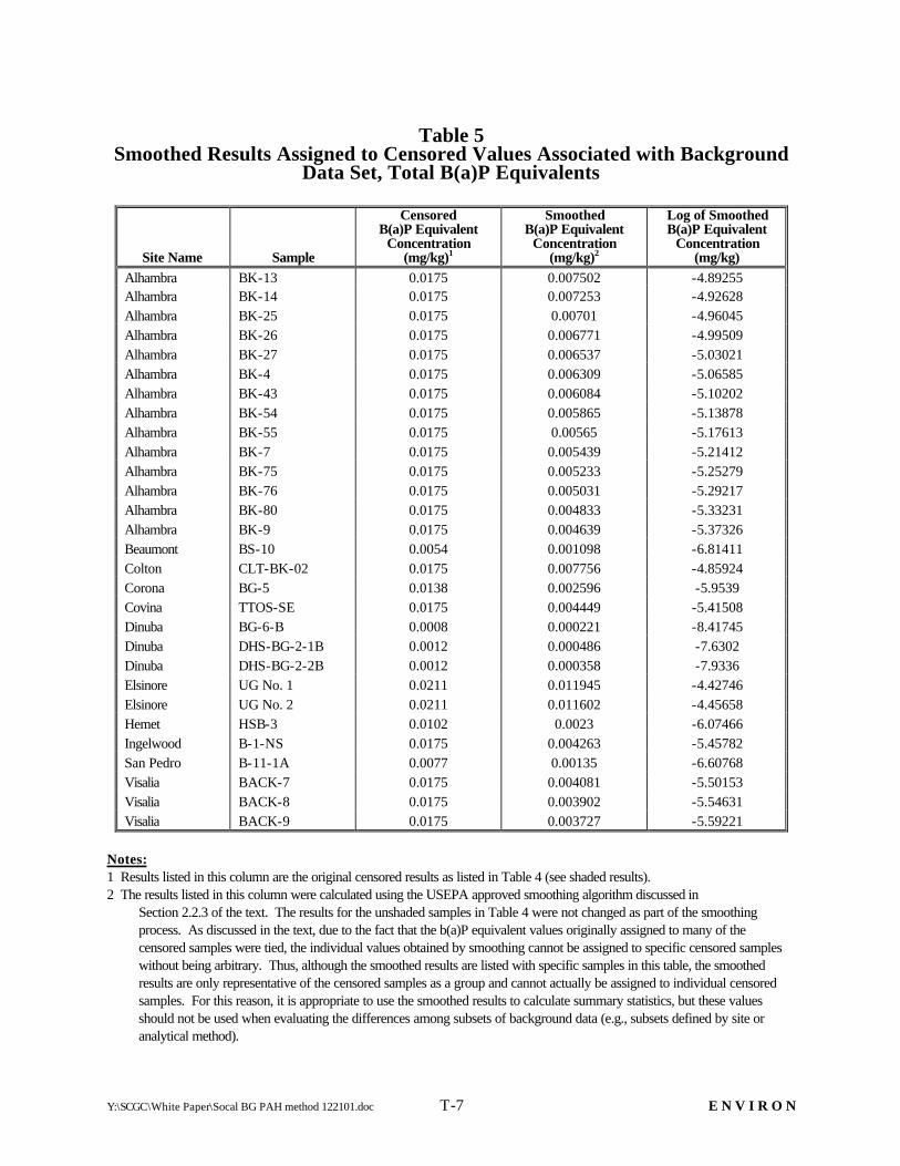
Y:\SCGC\White Paper\Socal BG PAH method 122101.doc T-7 E N V I R O N
Table 5 Smoothed Results Assigned to Censored Values Associated with Background
Data Set, Total B(a)P Equivalents
Site Name Sample
Censored B(a)P Equivalent
Concentration (mg/kg)1
Smoothed B(a)P Equivalent
Concentration (mg/kg)2
Log of Smoothed B(a)P Equivalent
Concentration (mg/kg)
Alhambra BK-13 0.0175 0.007502 -4.89255 Alhambra BK-14 0.0175 0.007253 -4.92628 Alhambra BK-25 0.0175 0.00701 -4.96045 Alhambra BK-26 0.0175 0.006771 -4.99509 Alhambra BK-27 0.0175 0.006537 -5.03021 Alhambra BK-4 0.0175 0.006309 -5.06585 Alhambra BK-43 0.0175 0.006084 -5.10202 Alhambra BK-54 0.0175 0.005865 -5.13878 Alhambra BK-55 0.0175 0.00565 -5.17613 Alhambra BK-7 0.0175 0.005439 -5.21412 Alhambra BK-75 0.0175 0.005233 -5.25279 Alhambra BK-76 0.0175 0.005031 -5.29217 Alhambra BK-80 0.0175 0.004833 -5.33231 Alhambra BK-9 0.0175 0.004639 -5.37326 Beaumont BS-10 0.0054 0.001098 -6.81411 Colton CLT-BK-02 0.0175 0.007756 -4.85924 Corona BG-5 0.0138 0.002596 -5.9539 Covina TTOS-SE 0.0175 0.004449 -5.41508 Dinuba BG-6-B 0.0008 0.000221 -8.41745 Dinuba DHS-BG-2-1B 0.0012 0.000486 -7.6302 Dinuba DHS-BG-2-2B 0.0012 0.000358 -7.9336 Elsinore UG No. 1 0.0211 0.011945 -4.42746 Elsinore UG No. 2 0.0211 0.011602 -4.45658 Hemet HSB-3 0.0102 0.0023 -6.07466 Ingelwood B-1-NS 0.0175 0.004263 -5.45782 San Pedro B-11-1A 0.0077 0.00135 -6.60768 Visalia BACK-7 0.0175 0.004081 -5.50153 Visalia BACK-8 0.0175 0.003902 -5.54631 Visalia BACK-9 0.0175 0.003727 -5.59221
Notes: 1 Results listed in this column are the original censored results as listed in Table 4 (see shaded results). 2 The results listed in this column were calculated using the USEPA approved smoothing algorithm discussed in
Section 2.2.3 of the text. The results for the unshaded samples in Table 4 were not changed as part of the smoothing process. As discussed in the text, due to the fact that the b(a)P equivalent values originally assigned to many of the censored samples were tied, the individual values obtained by smoothing cannot be assigned to specific censored samples without being arbitrary. Thus, although the smoothed results are listed with specific samples in this table, the smoothed results are only representative of the censored samples as a group and cannot actually be assigned to individual censored samples. For this reason, it is appropriate to use the smoothed results to calculate summary statistics, but these values should not be used when evaluating the differences among subsets of background data (e.g., subsets defined by site or analytical method).

Y:\SCGC\White Paper\Socal BG PAH method 122101.doc T-8 E N V I R O N
Table 6 Point Estimates of PAH Background Concentration in Soil Derived
from Smoothed Background Data Set
Summary Statistic Value (mg/kg, B(a)P Equivalents)
95th percentile 0.61 Upper Tolerance Limit (UTL) 95% coverage, 95% confidence 0.90 Upper Prediction Limit (UPL) 95% Confidence, 5 samples 2.0

FIGURE 1: Location of Southern California MGP Sites from which Background Samples were Collected


Y:\SCGC\White Paper\Att A.doc 1
ATTACHMENT A Calculation of Risk-Based Soil Concentrations for PAHs in Soil
1.0 Introduction
This attachment describes the methodology and assumptions used to calculate risk-based concentrations (RBCs) for benzo(a)pyrene (B(a)P) in soil. As is shown below, the RBC for carcinogenic PAHs, expressed in B(a)P equivalents calculated assuming unrestricted land use (e.g., a single family residential exposure scenario) are lower than background levels. B(a)P soil RBCs calculated for a commercial/industrial worker exposure scenario or an intrusive worker exposure scenario are higher than cleanup goals calculated for a residential exposure scenario and are higher than typical background levels. The following sections present RBCs calculations for B(a)P in soil under three different assumed exposure scenarios (i.e., unrestricted residential, industrial/commercial worker, and intrusive worker). These RBCs can be compared to PAH background levels to support remediation decisions.
The remaining sections of this attachment describe the methodology used to derive population-specific human health RBCs for B(a)P in soil and are organized as follows: Section 2.0 describes the methodology and guidelines used to develop B(a)P soil RBCs; Section 3.0 describes potentially exposed populations, potential exposure pathways and routes, and population-specific exposure assumptions; Section 4.0 describes chronic toxicity assessment of carcinogenic and noncarcinogenic effects; Section 5.0 describes mathematical equations used to calculate B(a)P soil RBCs; and Section 6.0 lists the references cited in this attachment.
2.0 Derivation of Human Health Risk-based Concentrations for PAHs in Soil
RBCs are health-based, chemical-specific concentrations used to support evaluations of whether contaminants are present at concentrations that raise concern for human health. RBCs are calculated based on the health effects of individual chemicals in specific media (e.g., soil) and land-use combinations at a site. RBCs are developed to be protective of people potentially exposed to site-related chemicals in soil and are developed for individual chemicals, specific media, and exposure scenarios for both carcinogenic and noncarcinogenic health effects.
The general methodology used to develop RBCs follows State and Federal guidance for risk assessment and calculation of chemical-specific media cleanup levels including:
• Risk Assessment Guidance for Superfund, Volume 1, Human Health Evaluation Manual (Part A) (USEPA 1989)
• Risk Assessment Guidance for Superfund, Volume 1, Human Health Evaluation Manual (Part B, Development of Risk-Based Preliminary Remediation Goals) (USEPA 1991b)
• Supplemental Guidance for Human Health Multimedia Risk Assessments of Hazardous Waste Sites and Permitted Facilities (Cal/EPA 1992)
The National Contingency Plan (NCP) (40 CFR § 300) is commonly cited as the basis for target risk levels. According to the NCP, lifetime incremental cancer risks posed by a site should not exceed one

Y:\SCGC\White Paper\Att A.doc 2
in a million (1 x 10⁻⁶) to one hundred in a million (1 x 10⁻⁴), and noncarcinogenic chemicals should not be present at levels expected to cause adverse health effects (i.e., hazard index (HI) greater than 1). As a risk management policy, the Cal/EPA generally requires risks to be closer to the 1 x 10⁻⁶ end of the target risk range, with most approved remediations achieving incremental risk levels of ten in a million (1 x 10⁻⁵) or lower. For this risk assessment the target cancer risk used for the calculation of RBCs for carcinogens is one in one million (1 x 10⁻⁶). The target HI used for the calculation of RBCs for noncarcinogens is 1.
3.0 Exposure Assessment
In evaluating the potential health risks posed by a Site, it is necessary to identify the populations that may potentially be exposed to site-related contaminants and to determine the pathways by which these exposures may occur. Identification of the potentially exposed populations requires evaluating the human activity and land-use patterns at and in the vicinity of the Site.
Once the potentially exposed populations are identified, the complete exposure pathways by which individuals in each of these populations may contact site-related contaminants are determined. An exposure pathway is defined as “the course a chemical or pollutant takes from the source to the organism exposed” (USEPA 1988). An exposure route is “the way a chemical or pollutant enters an organism after contact” (USEPA 1988). A complete exposure pathway requires four key elements:
• On-site chemical sources;
• Migration routes (e.g., environmental transport);
• Exposure point for contact (e.g., soil, air, or water); and
• Human exposure routes (e.g., oral, dermal, inhalation).
An exposure pathway is not complete unless all four elements are present.
3.1 Potentially Exposed Populations
Three potentially exposed populations have been selected as the basis for B(a)P soil RBCs. These include a commercial/industrial worker, a maintenance/construction worker, and a resident. Consistent with the historic and intended future land use of many former MGP Sites as service base centers, or as other commercial/industrial centers, workers have been selected as one potentially exposed population. These are workers who would work at the Site but who typically would not have occasion to engage in soil excavation activities involving direct contact with surface and subsurface soils. Because there will certainly be a need for maintenance/construction activities, such as digging through the soil for such activities as maintenance and repair of utilities, construction workers have been selected as another potentially exposed population. The activities of this population are expected to involve intrusive soil work resulting in direct contact with surface and subsurface soil. Since in many instances the most desired goal of any remedial action is to prepare a site for potential future residential land use, we have selected hypothetical future residents as a potentially exposed population. The RBCs calculated for residents under an unrestricted residential land use will provide cleanup levels for evaluating the potential unrestricted use of the Site in the future.

Y:\SCGC\White Paper\Att A.doc 3
3.2 Potential Exposure Pathways and Routes
The commercial/industrial workers, construction/maintenance workers, and residents could be exposed to PAHs in the soil through the following pathways:
• Surface soil –incidental ingestion, dermal contact, and inhalation of airborne soil particulates (all potentially exposed populations);
• Subsurface soil – incidental ingestion, dermal contact, and inhalation of airborne soil particulates (construction workers and potential future residents).
Construction workers engaged in intrusive projects could also be exposed to subsurface soil via ingestion, dermal contact, and inhalation of particulates. Similarly, when assessing potential future residential exposures, it is conservatively assumed that subsurface soils could be excavated and spread across the site (e.g., during construction of a swimming pool) and thus future residents could potentially be exposed to subsurface soils via ingestion, dermal contact, and inhalation of particulates. Commercial workers are assumed not to have direct contact with subsurface soil.
3.3 Exposure Assumptions
When available, Cal/EPA and USEPA recommendations for exposure assumptions were used to estimate intakes from each environmental media for each potentially exposed population. When specific recommendations were not available, ENVIRON used methods described in State and Federal guidance, and conservative judgment to develop exposure assumptions appropriate for the Site. Route-specific exposure assumptions are presented in Table 1 along with the source or rationale for selecting each of the assumptions.
3.4 Population-Specific Intake Factors
As described above, exposures to the potentially exposed populations evaluated in this attachment may result from soil ingestion, dermal contact, and inhalation of airborne soil particulates. Route-specific intake factors are based on the total amount of soil each population contacts over the specified period of exposure. Intake factors for each potentially exposed population are presented in Table 2. The route-specific intake factors listed in Table 2 were calculated using the following equation:
ATBW
EDEFIR
×××=FI
where:
IF = Intake: the amount of chemical at the exchange boundary (that is, lungs skin, or gastrointestinal tract; kg soil/kg body weight-day); IR = Intake rate: the amount of contaminated medium contacted per unit of

Y:\SCGC\White Paper\Att A.doc 4
time or event (e.g., dermal intake rate = surface area * adherence factor
* absorption factor * conversion factor); EF = Exposure frequency: how often the exposure occurs (days per year) ED = Exposure duration: the number of years that a receptor comes in
contact with the contaminated medium (years) BW = Body weight: the average body weight of the receptor over the
exposure period (kg) AT = Averaging time: the period over which exposure is averaged (years);
for carcinogens, the averaging time is based on a lifetime exposure of 70 years (average life expectancy), and for noncarcinogens, the averaging time is equal to the exposure duration.
4.0 Dose-Response Assessment
Dose-response assessment is the process of characterizing the relationship between the exposure to a chemical and the incidence of adverse health effects in exposed populations. Chemicals are usually evaluated for their potential health effects in two categories, carcinogenic and noncarcinogenic. Different methods are used to evaluate the potential for these two types of health effects. Chemicals that produce carcinogenic effects may also produce noncarcinogenic effects. The USEPA and Cal/EPA consider carcinogens to pose a risk for cancer at all exposure levels (i.e., a "no-threshold" assumption); that is, any increase in dose over background is associated with an increase in the probability of developing cancer. In contrast, noncarcinogens generally are thought to produce adverse health effects only when some minimum exposure level is reached (i.e., a threshold dose).
The hierarchy of sources for the toxicity criteria used in development of the RBCs correspond to the State's guidelines as follows (Cal/EPA 1994a):
• California promulgated cancer slope factors (CSFs), as listed in the most recent Cancer Potency Factors memo, which is periodically updated (Cal/EPA 1994b);
• CSFs, Reference Doses (RfDs), and Reference Concentrations (RfCs) developed by the USEPA and listed in the Integrated Risk Information Service (IRIS) (USEPA 2001);
• USEPA CSFs, RfDs, and RfCs listed in the USEPA Health Effects Assessment Summary Tables (HEAST) (USEPA 1997); and
• Provisional USEPA RfDs and RfCs recommend by USEPA's National Center for Environmental Assessment (NCEA).
The following sections describe the methods used for the toxicity assessment of carcinogens and noncarcinogens, respectively. The toxicity values used to develop the B(a)P soil RBCs presented in this attachment are presented in Table 3.
Y:\SCGC\White Paper\Att A.doc 5
4.1 Chronic Toxicity Assessment for Carcinogenic Effects
Current health risk assessment practice for carcinogens is based on the assumption that there is no threshold dose below which carcinogenic effects do not occur. This current "no-threshold" assumption for carcinogenic effects is based on an assumption that the carcinogenic processes are the same at high and low doses. This approach has generally been adopted by regulatory agencies as a conservative practice to protect public health. The "no-threshold" assumption is used in this evaluation for assessing carcinogenic effects. Although the magnitude of the risk declines with decreasing exposure, the risk is believed to be zero only at zero exposure.
CSFs are used to quantify a chemical’s carcinogenic potency. CSFs are usually derived from toxicological studies using animal species. There are a large number of uncertainties associated with the derivation of these values, including the difficulties in extrapolation from toxicity in animals to that in humans, from the length of a study to a human lifetime, and predicting chemical toxicity at lower doses. To account for these uncertainties, a conservative model is used in the derivation of CSFs. The CSF represents the excess lifetime cancer risk due to a continuous, constant lifetime exposure to a specified level of a carcinogen. CSFs are generally reported as excess incremental cancer risk per milligram of chemical per kilogram body weight per day (mg/kg/day)-1.
Specific dermal route toxicity factors have not yet been developed for any chemicals. Consistent with USEPA (1989) and Cal/EPA (1994a) guidance, dermal risk has been calculated using oral toxicity factors.
4.2 Chronic Toxicity Assessment for Noncarcinogenic Effects
The dose-response assessment for noncarcinogenic effects requires the derivation of an exposure level below which no adverse health effects in humans are expected to occur. USEPA refers to these levels as reference doses (RfDs) for oral exposure and reference concentrations (RfCs) for inhalation exposure (USEPA 1989). When available, USEPA-derived oral RfDs and inhalation RfCs are used to evaluate the noncarcinogenic effects. RfDs and RfCs are usually derived from toxicological studies using animal species. There are a large number of uncertainties associated with the derivation of these values, including extrapolation from toxicity in animals to that in humans, the extrapolation from the length of a study to a human lifetime, and the extrapolation from levels at which a toxic effect is seen to levels that would cause no effect. For this reason, an uncertainty factor between 10 and 10,000 is typically included in the calculation of RfDs and RfCs. RfDs are obtained from IRIS, HEAST, or other USEPA or CalEPA guidance. For the characterization of the potential noncarcinogenic health effects, inhalation RfCs, which the USEPA generally reports as concentrations in air, are converted to corresponding inhaled doses (inhalation RfDs) using USEPA-approved interim methodology (USEPA 1989). Noncarcinogenic effects associated with dermal routes of exposure are evaluated using the oral RfDs, as recommended by USEPA (1989) and Cal/EPA (1994a).
5.0 Risk-Based Concentrations
The B(a)P soil RBCs presented in this attachment represent the concentrations of B(a)P which could remain in the soil without posing a significant human health risk to current and future populations.

Y:\SCGC\White Paper\Att A.doc 6
Uncertainties regarding the exposure assumptions, correlation/particulate emission factors, and toxicity values are inherent in the calculation of the RBCs.
RBCs for B(a)P in soil were calculated for residents and workers on the Site. Exposure was assumed to occur through incidental ingestion, dermal contact, and inhalation of airborne particulates and vapors. The equations used to calculate RBCs for the individuals exposed via ingestion, dermal contact, and inhalation are as follows:
])[IF(CSF]IF )[IF(CSFRiskCancer Target
RBCinhalinhaldermaloraloral
Carcinogen++
=
RfD
) IF + (IF +
RfD
)(IFIndex HazardTarget
= RBC
oral
dermaloral
Inhalation
InhalationgenNoncarcino
where:
CSFinhal = Inhalation cancer slope factor, as specified by Cal/EPA (1994b) or IRIS, (mg chemical/kg body weight-day)-1;
IFinhal = Route-specific intake equation for inhalation of particulates or vapors (kg soil/kg-body weight-day).
CSForal = Oral cancer slope factor, as specified by Cal/EPA (1994b) or IRIS, (mg chemical/kg body weight-day)-1;
IFing = Route-specific intake equation for soil ingestion, (kg soil/kg-body weight-day);
IFderm = Route-specific intake equation for dermal contact, (kg soil/kg-body weight-day);
RfDinhal = Inhalation reference dose, the toxicity value indicating the threshold amount of chemical contacted below which no adverse health effects are expected, (mg chemical/kg body weight-day);
RfDoral = Oral reference dose, the toxicity value indicating the threshold amount of chemical contacted below which no adverse health effects are expected, (mg chemical/kg body weight-day).
B(a)P soil RBCs were calculated for both carcinogenic effects (Table 4) and noncarcinogenic effects (Table 5). The lower of the population- specific carcinogenic and noncarciongenic B(a)P soil RBCs should be used as remedial action goals when evaluating potential risks to human health associated with former MGP sites. The lowest B(a)P soil RBCs corresponding to several target risk levels for each potentially exposed population are presented in Table 6.

Y:\SCGC\White Paper\Att A.doc 7
6.0 References California Environmental Protection Agency (Cal/EPA). 1992. Department of Toxic Substances
Control (DTSC). Supplemental Guidance for Human Health Multimedia Risk Assessment of Hazardous Waste Sites and Permitted Facilities. Sacramento, CA. July.
California Environmental Protection Agency (Cal/EPA). 1994a. Department of Toxic Substances
Control (DTSC). Preliminary Endangerment Assessment Guidance Manual. State of California Environmental Protection Agency. January.
California Environmental Protection Agency (Cal/EPA). 1994b. Memorandum, to Cal/EPA
Departments, Boards, and Offices from Standards and Criteria Work Group, Office of Environmental Health Hazard Assessment. Subject: California Cancer Potency Factors. November 1.
Code of Federal Regulations (CFR). 1997. Title 40, Environmental Protection Agency (EPA). Part
300, National Oil and Hazardous Substances Pollution Contingency Plan. July 1. (40 CFR § 300)
ENVIRON, 1998. A Methodology for Using Background PAHs to Support Remediation Decisions.
Prepared for Southern California Gas Company and Southern California Edison. March. U.S. Environmental Protection Agency (USEPA). 1988. Superfund Exposure Assessment Manual.
EPA/540/1-88/001. Washington, D.C. April. U.S. Environmental Protection Agency (USEPA). 1989. Risk Assessment Guidance for Superfund.
Volume 1: Human Health Evaluation Manual (Part A). Office of Emergency and Remedial Response.EPA/540/1-89/002. December.
U.S. Environmental Protection Agency (USEPA). 1991a. Risk Assessment Guidance for Superfund.
Volume 1: Human Health Evaluation Manual. Supplemental Guidance. Standard Default Exposure Factors. Office of Emergency and Remedial Response, Toxics Integration Branch. March 25.
U.S. Environmental Protection Agency (USEPA). 1991b. Risk Assessment Guidance for Superfund.
Volume I- Human Health Evaluation Manual. (Part B, Development of Risk-Based Preliminary Remediation Goals). Publication 9285.701B.
U.S. Environmental Protection Agency (USEPA). 1997a. Health Effects Assessment Summary Tables.
Annual FY 1997. Office of Research and Development. U.S. Environmental Protection Agency (USEPA). 1997b. Exposure Factors Handbook. Volume I –
General Factors. EPA/600/P-95/002Fa. Washington, D.C. August. U.S. Environmental Protection Agency (USEPA). 2000. Region 9 Preliminary Remediation Goals.
Introduction. San Francisco, CA. November.

Y:\SCGC\White Paper\Att A.doc 8
U.S. Environmental Protection Agency (USEPA). 2001. Integrated Risk Information System (IRIS). Office of Research and Development. Office of Health and Environmental Assessment.
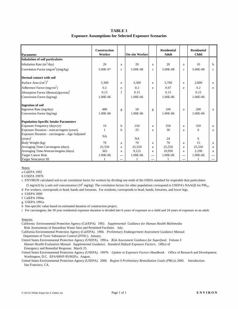
TABLE 1Exposure Assumptions for Selected Exposure Scenarios
ParameterConstruction
Worker On-site WorkerResidential
AdultResidential
ChildInhalation of soil particulates
Inhalation Rate (m3/day) 20 a 20 a 20 a 10 b
Correlation Factor (mg/m3)/(mg/kg) 5.00E-07 c 5.00E-08 c 5.00E-08 c 5.00E-08 c
Dermal contact with soil
Surface Area (cm2)d 3,300 e 3,300 e 5,700 e 2,800 e
Adherence Factor (mg/cm2) 0.2 e 0.2 e 0.07 e 0.2 eAbsorption Factor (Benzo(a)pyrene)f 0.15 f 0.15 0.15 0.15Conversion Factor (kg/mg) 1.00E-06 1.00E-06 1.00E-06 1.00E-06
Ingestion of soilIngestion Rate (mg/day) 480 g 50 g 100 a 200 aConversion Factor (kg/mg) 1.00E-06 1.00E-06 1.00E-06 1.00E-06
Population-Specific Intake ParametersExposure Frequency (days/yr) 10 h 250 a 350 a 350 aExposure Duration - noncarcingens (years) 1 h 25 a 30 a 6 aExposure Duration - carcinogens - Age-Adjusted (years)i NA
NA 24 6Body Weight (kg) 70 a 70 a 70 a 15 aAveraging Time-Carcinogens (days) 25,550 a 25,550 a 25,550 a 25,550 aAveraging Time-Noncarcinogens (days) 365 a 9,125 a 10,950 a 2,190 aTarget Cancer Risk 1.00E-06 --- 1.00E-06 --- 1.00E-06 --- 1.00E-06 ---Target Noncancer HI 1 --- 1 --- 1 --- 1 ---
Notes:a CalEPA 1992b USEPA 1997bc ENVIRON calculated soil-to-air correlation factor for workers by dividing one tenth of the OSHA standard for respirable dust particulates
(5 mg/m3) by a unit soil concentration (106 mg/kg). The correlation factors for other populations correspond to USEPA's NAAQS for PM10.d For workers, corresponds to head, hands and forearms. For residents, corresponds to head, hands, forearms, and lower legs.e USEPA 2000f CalEPA 1994ag USEPA 1991ah Site-specific value based on estimated duration of construction project.i For carcinogens, the 30 year residential exposure duration is divided into 6 years of exposure as a child and 24 years of exposure as an adult.
Sources:California Environmental Protection Agency (Cal/EPA). 1992. Supplemental Guidance for Human Health Multimedia Risk Assessments of Hazardous Waste Sites and Permitted Facilities. July. California Environmental Protection Agency (Cal/EPA). 1994. Preliminary Endangerment Assessment Guidance Manual. Department of Toxic Substances Control (DTSC). January.United States Environmental Protection Agency (USEPA). 1991a. Risk Assessment Guidance for Superfund. Volume I: Human Health Evaluation Manual. Supplemental Guidance. Standard Default Exposure Factors. Office of Emergency and Remedial Response. March 25.United States Environmental Protection Agency (USEPA). 1997b. Update to Exposure Factors Handbook. Office of Research and Development. Washington, D.C. EPA/600/P-95/002Fa. August.United States Environmental Protection Agency (USEPA). 2000. Region 9 Preliminary Remediation Goals (PRGs) 2000. Introduction. San Francisco, CA.
Y:\SCGC\White Paper\Att A Table1.xls Page 1 of 1 E N V I R O N
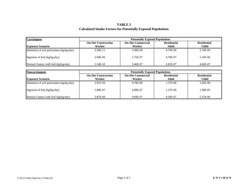
TABLE 2Calculated Intake Factors for Potentially Exposed Populations
Carcinogens Potentially Exposed PopulationsOn-Site Construction On-Site Commercial Residential Residential
Exposure Scenario Worker Worker Adult ChildInhalation of soil particulates (kg/kg-day) 5.59E-11 3.49E-09 4.70E-09 2.74E-09
Ingestion of Soil (kg/kg-day) 2.68E-09 1.75E-07 4.70E-07 1.10E-06
Dermal Contact with Soil (kg/kg-day) 5.54E-10 3.46E-07 2.81E-07 4.60E-07
Noncarcinogens Potentially Exposed PopulationsOn-Site Construction On-Site Commercial Residential Residential
Exposure Scenario Worker Worker Adult ChildInhalation of soil particulates (kg/kg-day) 3.91E-09 9.78E-09 1.37E-08 3.20E-08
Ingestion of Soil (kg/kg-day) 1.88E-07 4.89E-07 1.37E-06 1.28E-05
Dermal Contact with Soil (kg/kg-day) 3.87E-08 9.69E-07 8.20E-07 5.37E-06
Y:\SCGC\White Paper\Att A Table2.xls Page 1 of 1 E N V I R O N

TABLE 3Carcinogenic and Noncarcinogenic Toxicity Values
Weight of
Cancer Slope Factor(mg/kg-d)-1
Noncancer Reference Dose(mg/kg-d)
Chemical Evidence oral source inhalation source Chemical oral source inhalation source
Benzo(a)pyrene B2 1.20E+01 Cal/EPA 1994 3.90E+00 Cal/EPA 1994 Naphthalenea 2.00E-02 IRIS 8.57E-04 IRIS
Notes:a Toxicity values for naphthalene used as a surrogate for noncancer effects associated with all PAHs.
Sources:Cal/EPA 1994 - California Environmental Protection Agency (Cal/EPA). 1994. Memorandum: California Cancer Potency Factors: Update. San Francisco, CA. November 1.IRIS - U.S. Environmental Protection Agency (USEPA). 2001. Integrated risk information system (IRIS). Online database maintained by USEPA. Cincinnati, OH.
Y:\SCGC\White Paper\Att A Table3.xls Page 1 of 1 E N V I R O N
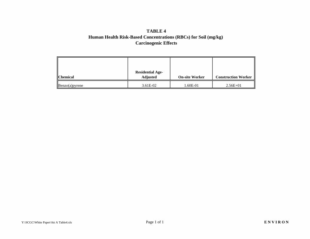
TABLE 4Human Health Risk-Based Concentrations (RBCs) for Soil (mg/kg)
Carcinogenic Effects
ChemicalResidential Age-
Adjusted On-site Worker Construction Worker
Benzo(a)pyrene 3.61E-02 1.60E-01 2.56E+01
Y:\SCGC\White Paper\Att A Table4.xls Page 1 of 1 E N V I R O N

TABLE 5Human Health Risk-Based Concentrations (RBCs) for Soil (mg/kg)
Non-Carcinogenic Effects
ChemicalConstruction Worker On-site Worker Residential Adult Residential Child
Naphthalenea 6.29E+04 1.19E+04 7.97E+03 1.06E+03
Notes:a Toxicity values for naphthalene used as a surrogate for noncancer effects associated with all PAHs.
Y:\SCGC\White Paper\Att A Table5.xls Page 1 of 1 E N V I R O N

TABLE 6Lowest Human Health Risk-Based Concentrations (RBCs) for Soil (mg/kg)
Potentially Exposed Populations
Resident On-site Worker Construction Worker
Risk Level Risk Level Risk Level
Chemical 1 x 10⁻⁶ 1 x 10⁻⁵ 1 x 10⁻⁴ 1 x 10⁻⁶ 1 x 10⁻⁵ 1 x 10⁻⁴ 1 x 10⁻⁶ 1 x 10⁻⁵ 1 x 10⁻⁴
Benzo(a)pyrene (and equivalents) 3.61E-02 C 3.61E-01 C 3.61E+00 C 1.60E-01 C 1.60E+00 C 1.60E+01 C 2.56E+01 C 2.56E+02 C 2.56E+03 C
Notes:C = RBC for carcinogenic effects.
Y:\SCGC\White Paper\Att A Table6.xls Page 1 of 1 E N V I R O N