a methodology for snow data assimilation in a land surface ... · a methodology for snow data...

A methodology for snow data assimilation in a land surface model

Chaojiao Sun1

Hydrological Sciences Branch, Laboratory for Hydrospheric Processes, NASA Goddard Space Flight Center, Greenbelt,Maryland, USA

Goddard Earth Sciences and Technology Center, University of Maryland Baltimore County, Baltimore, Maryland, USA

Jeffrey P. WalkerDepartment of Civil and Environmental Engineering, University of Melbourne, Parkville, Victoria, Australia

Paul R. HouserHydrological Sciences Branch, Laboratory for Hydrospheric Processes, NASA Goddard Space Flight Center, Greenbelt,Maryland, USA

Received 11 May 2003; revised 4 March 2004; accepted 22 March 2004; published 27 April 2004.

[1] Snow cover has a large influence on heat fluxes between the land and atmospherebecause of its high albedo and insulating thermal properties. Hence accurate snowrepresentation in coupled land-ocean-atmosphere global climate models has the potentialto greatly increase prediction accuracy. To this end, a one-dimensional extended Kalmanfilter analysis scheme has been developed to assimilate observed snow water equivalentinto the NASA Seasonal-to-Interannual Prediction Project (NSIPP) catchment-basedland surface model. This study presents the results from a set of data assimilation ‘‘twin’’experiments using an uncoupled version of the land surface model. First, ‘‘true’’ snowstates are generated by spinning-up the land surface model for 1987 using an observation-constrained version of the European Centre for Medium-Range Weather Forecasts(ECMWF) 15-year Re-Analysis (ERA-15) data set for atmospheric forcing. A degraded1987 simulation was then made by initializing the model with no snow on 1 January 1987.A third simulation assimilated the synthetically generated snow water equivalent‘‘observations’’ from the true simulation into the degraded simulation once a day. Thisstudy illustrates that by assimilating snow water equivalent observations, which are readilyavailable from remote sensing satellites, other state variables (i.e., snow depth andtemperature) can be retrieved and effects of poor initial conditions removed. Runoff andatmospheric flux predictions are also improved. INDEX TERMS: 1863 Hydrology: Snow and ice

(1827); 3260 Mathematical Geophysics: Inverse theory; 3322 Meteorology and Atmospheric Dynamics: Land/

atmosphere interactions; 3337 Meteorology and Atmospheric Dynamics: Numerical modeling and data

assimilation; 3360 Meteorology and Atmospheric Dynamics: Remote sensing; KEYWORDS: snow assimilation,

extended Kalman filter, GCM initialization

Citation: Sun, C., J. P. Walker, and P. R. Houser (2004), A methodology for snow data assimilation in a land surface model,

J. Geophys. Res., 109, D08108, doi:10.1029/2003JD003765.

1. Introduction

1.1. Importance of Snow

[2] Snow plays an important role in governing the Earth’sglobal energy and water budgets, as a result of its highalbedo, low thermal conductivity, and considerable spatialand temporal variability [Hall, 1998]. Snow cover is one ofthe most highly varying hydrological quantities on theEarth’s surface [Gutzler and Rosen, 1995], with the North-ern Hemisphere mean monthly snow covered land area

ranging from about 7% to 40% during the annual cycle[Hall, 1988]. Moreover, the energy demanded by snowmeltcan significantly cool the surface and the overlying air[Dewey, 1977; Namias, 1985; Baker et al., 1992; Groismanet al., 1994]. Thus surface air temperature forecasts fromnumerical weather prediction are very sensitive to the snowcover extent and thickness. For example, improvement ofsnow physics in the NCEP (National Centers for Environ-mental Prediction) ETA operational forecast model substan-tially reduced a 2 m daytime air temperature cold bias forsnow covered areas [Mitchell et al., 2002]. Further, snowcovered landscapes adjacent to bare soil regions have beenfound to produce mesoscale wind circulations [Johnson etal., 1984] and snow cover variability has been shown toaffect climate patterns in coupled climate simulations. Using

JOURNAL OF GEOPHYSICAL RESEARCH, VOL. 109, D08108, doi:10.1029/2003JD003765, 2004

1Now at Global Modeling and Assimilation Office, NASA GoddardSpace Flight Center, Greenbelt, Maryland, USA.

Copyright 2004 by the American Geophysical Union.0148-0227/04/2003JD003765$09.00

D08108 1 of 12

the NESDIS (National Environmental Satellite, Data, andInformation Service) snow cover data [Robinson et al.,1993], Cohen and Entekhabi [1999] demonstrate that earlyseason Eurasian snow cover variations are associated withdominant modes of midlatitude variability in the NorthernHemisphere winter. In addition, recent observational studies[Lo and Clark, 2002; Bamzai and Shukla, 1999] haveshown an inverse relationship between antecedent snowmass or snow cover extent and Asian and North Americansummer monsoon intensity. Hence any long term coupledclimate system prediction is dependent on accurate snowinformation.[3] Because of its low thermal conductivity, snow can

insulate the underlying soil and impede the depth andseverity of soil freezing [Lynch-Stieglitz, 1994; Sud andMocko, 1999]. While the energy balance is the primarydriver of the Earth’s atmospheric circulation system andassociated climate, the water budget is also significantlymodified through snowmelt processes. Being a medium-term water store, snow plays an important role in springtimerunoff generation and flood production [Hall, 1988], andcan provide a substantial component of the annual waterbudget. In many northern latitude regions (e.g., California),spring meltwater from the winter snowpack is the greatestsource of water in the annual soil moisture budget [Aguado,1985]. Therefore, to achieve accurate runoff and soil mois-ture prediction, which provides feedback to climate predic-tion [Koster and Suarez, 1995], it is important to accuratelyinitialize snow cover in climate model forecasts.

1.2. Snow Observations

[4] Owing to considerable subgrid-scale spatial and tem-poral snow variability, and deficiencies in model snowphysics, realistic global climate model snow prediction isdifficult [Liston et al., 1999]. Any land surface modelinitialization based solely on model spin-up will be affectedby these problems. While there is a demonstrated need forroutine snow observation (snow water equivalent, snowdepth, snow temperature and hence snow cover), particu-larly for climate model initialization, routine ground-basedsnow observations are uncommon. In the United States,daily snow depth measurements are available at airports andfrom a network of volunteer observers. Snow course andSNOTEL (Snowpack Telemetry) sites collect more detailedsnow data (snow depth, snow water equivalent and snowtemperature), but these data are only collected in remoteareas of the mountainous western states (information onSNOTEL can be found on the following Web site: http://www.wcc.nrcs.usda.gov/snotel/). In Canada, daily ground-based snow depth observations have been made at mostsynoptic stations since the 1950s, but the observing networkis concentrated over the southern, more populated regions.Snow course observations are widely distributed throughoutall of the provinces and territories, but they are madeinfrequently (weekly, biweekly or monthly) [Brown et al.,2003]. Even though the in situ North American observationsare among the best in the world, they are insufficient forglobal climate model initialization due to extreme snowdepth heterogeneity.[5] In contrast, remote sensing has the capability for

providing snow information with the spatial coverage andtemporal resolution needed for global climate model initial-

ization. Remote sensing observations average out the small-scale variability inherent to in situ snow observations,therefore producing better climate-relevant snow informa-tion. Operational weekly snow cover analyses over NorthAmerica have been produced from visible satellite obser-vations by NOAA since 1966 [Robinson et al., 1993].Although this is the longest remotely sensed snow recordavailable, it only provides the snow cover rather than snowmass information. While visible-infrared satellite sensors,such as the Moderate Resolution Imaging Spectroradiom-eter (MODIS) onboard Terra and Aqua currently providethe highest daily snow cover spatial resolution (500 m),they only work for cloud-free conditions. These high-resolution observations can provide information on frac-tional coverage of snow, which complements passivemicrowave observations that have coarser resolution, butfractional snow cover observation alone is difficult to usefor quantitative snowpack initialization. Infrared sensorscan also provide surface skin temperature information forcloud free areas. However, these temperature observationsmay not represent the surface snow temperature, especiallywhen vegetation protrudes above the snowpack. Whenhigh-resolution snow cover and surface skin temperatureobservations are used together with snow mass observa-tions from passive microwave sensors, synergistic benefitsmay be derived for estimating snowpack states. Sinceresearch-quality data sets of simultaneous snow cover,snow depth, and snow water equivalent observations arestill under development [Robinson, 2002], we focus onusing passive microwave observations in this study.[6] Passive microwave sensors can measure snow mass

(snow water equivalent) under both nighttime and cloudy(nonprecipitating) conditions, which persist during muchof the high latitude snow season. Since November 1978,the Scanning Multichannel Microwave Radiometer(SMMR) and the Special Sensor Microwave Imager(SSM/I) have been acquiring passive microwave observa-tions. SMMR observations (resampled to 1=4 degree by 1=4degree resolution) are available from 1978 to 1987, andSSM/I observations (resampled to 1=2 degree by 1=2 degreeresolution) are available since 1987. With the launch ofthe Earth Observing System (EOS) Aqua satellite inMay 2002, high-quality passive microwave snow waterequivalent observations are available from its AdvancedMicrowave Scanning Radiometer for EOS (AMSR-E)instrument. AMSR-E is a passive microwave radiometerexpected to produce 10 km resolution snow water equiv-alent observations.[7] Chang et al. [1987] have developed a commonly

used algorithm to derive snow water equivalent and snowdepth from passive microwave data based on a radiativetransfer model with several assumptions. They assumedthat snow crystal size remains constant (0.3 mm) through-out the season. In reality, snow crystals evolve with theseason and weather conditions [Foster et al., 1997], andtheir size is the most important factor in determining thealgorithm accuracy. Vegetation cover can also imposelarge uncertainties in passive microwave snow waterequivalent estimation. For instance, Brown et al. [2001]showed that the boreal forest snowpack mass estimatedfrom passive microwave observations was consistentlyunderestimated. In a recent study, J. L. Foster et al.

D08108 SUN ET AL.: SNOW DATA ASSIMILATION

2 of 12

D08108

(Quantifying the uncertainty in passive microwave snowwater equivalent observations, submitted to Remote Sensingof Environment, 2004) have addressed these uncertaintiesand estimated errors in snow water equivalent observationsderived from passive microwave measurements, based onsnowpack age, climate, vegetation, topography, and bright-ness temperature measurement error. When the snowpack iswet, snow information is difficult to extract from passivemicrowave radiometry. Therefore only nighttime satelliteoverpasses are commonly examined, as there is a higherprobability that the snowpack is not actively melting atnight. Information on snowpack melt status, though notused in this study, could be used to further constrain modelsnow dynamics.

1.3. Snow Assimilation

[8] The few studies that have constrained model pre-dictions with snow observations have generally replacedthe modeled snow states with observations directly; thisassimilation method is commonly called ‘‘direct inser-tion.’’ For example, Liston et al. [1999] used this approachsuccessfully in identifying deficiencies in a regional cli-mate model associated with snow distribution, and Rodellet al. [2004] have used direct insertion to assimilateMODIS snow cover observations into the Global LandData Assimilation System (GLDAS). J. Jin and N. L.Miller (An analysis of climate variability and snowmeltmechanisms in mountainous regions, submitted to Journalof Hydrometeorology, 2003) also used this technique toinvestigate snowpack impact on climate variability andsnowmelt mechanisms in mountainous regions.[9] Direct insertion assumes that observations are perfect,

and model forecasts do not contain useful information.However, the reality is that model prediction can sometimesbe more accurate than observations; for example, model-predicted snow depth can be more accurate than remotelysensed observations in densely vegetated areas. The prop-agation of information to coupled state variables in directinsertion is accomplished only through model physics.B. A. Cosgrove and P. R. Houser (Impact of surface forcingbiases on snow assimilation, submitted to Journal ofHydrometeorology, 2003) found that large water balanceerrors occur when imperfectly modeled snow melting pro-cesses interact with the direct insertion of perfect snowobservations. Constraining these biases in assimilationsystems is important for achieving optimal assimilationresults [Dee and da Silva, 1998; Dee and Todling, 2000],and is an important topic for future research.[10] An improvement on direct insertion is the statistical

interpolation scheme (also called optimal interpolation).Brasnett [1999] used this scheme to assimilate snow depthobservations from synoptic stations into a very simplesnow accumulation, aging and melt model driven bynumerical weather prediction precipitation forecasts andscreen-level temperature analyses. The resulting globalsnow depth analysis was found to be more accurate thana climatological estimate. Recently, Brown et al. [2003]applied this method to generate a gridded monthly snowdepth and snow water equivalent data set for NorthAmerica, using snow depth observations from the UnitedStates cooperative stations and Canadian climate stations.They found that the gridded results agreed well with in

situ and satellite data over midlatitudinal regions during theAMIP II (Atmospheric Model Intercomparison Project II)period (1979–1996). These results provide impetus for thedevelopment of advanced assimilation methods and satelliteobservations to produce accurate snow fields for globalclimate model initialization.[11] In this study, we use the statistical Kalman filter

approach to assimilate snow water equivalent observations,which accounts for relative observation and predictionuncertainty to produce a statistically optimal estimate.We study the assimilation of satellite snow water equiva-lent observations made by passive microwave sensors,because snow water equivalent is crucial for estimatingwater fluxes in hydrologic models and surface albedo innumerical weather prediction models [Robinson andKukla, 1985]. Moreover, it is the total mass (i.e., snowwater equivalent, which is the product of snow depth anddensity) in the snowpack that directly determines itspassive microwave response; this is the basis for passivemicrowave snow water equivalent estimation. Thus for thisstudy we only assimilate remotely sensed snow waterequivalent, and allow the model to predict the snowdensity evolution. While directly replacing snow modelstate variables with observations is possible, this does notaccount for the relative prediction and observation errors,and does not provide a framework for correcting thenonobserved but highly correlated snow depth and heatcontent model state variables.[12] This study explores how routinely available passive

microwave snow water equivalent observations can beassimilated efficiently into a state-of-the-art land surfacemodel with a physically based snow submodel, using theextended Kalman filter. This methodology is developedthrough a series of numerical experiments using syntheticmodel-generated snow water equivalent observations. It isshown that sequential snow water equivalent assimilationcan also retrieve the snow depth and snow temperaturefields, and that runoff and atmospheric flux predictions areimproved.

2. Models

2.1. Land Surface Model

[13] This study uses the NASA Seasonal-to-InterannualPrediction Project (NSIPP) catchment-based land surfacemodel of Koster et al. [2000], which abandons thetraditional rectangular land surface discretization approachin favor of topographically based hydrological catchmentelements. The model includes an explicit subcatchment-scale soil moisture and evaporation variability treatmentwhere each catchment is divided into three regimes:saturated, stressed (wilting) and unstressed. In this appli-cation about 5000 catchments are used to model the NorthAmerican continent, with an average catchment size of3600 km2.[14] The forcing data for the catchment-based land

surface model, including air temperature and humidity at2 m height, wind speed at 10 m height, total andconvective precipitation, downward solar and longwaveradiation, and atmospheric pressure, were derived from the15-year (1979–1993) ECMWF Re-Analysis (ERA-15) thatwas scaled to match monthly averaged meteorological


3 of 12

D08108

observations [Berg et al., 2003]. Initial conditions wereobtained from ‘‘spinning-up’’ the catchment-based landsurface model by iterating the model over the same yearof atmospheric forcing for 10 years, by which time mostcatchments had reached equilibrium. The topographic, soiland vegetation parameter specifications are the same as inthe work of Walker and Houser [2001], with the catch-ment boundaries and topographic parameters derived froma 30 arc second (about 1 km) digital elevation model ofNorth America [Ducharne et al., 2000]. The soil andvegetation parameters are from the first InternationalSatellite Land Surface Climatology Project (ISLSCP) ini-tiative [Sellers et al., 1996].

2.2. Snow Submodel

[15] The catchment-based land surface model includes theLynch-Stieglitz [1994] snow submodel. This physicallybased snow model accounts for snowpack evaporation,sublimation, condensation, radiation interactions, precipita-tion as rain or snowfall depending on the air temperature,snowmelt, and metamorphosis [see also Stieglitz et al.,2001]. The snow model operates in both single-layer andthree-layer modes, depending on the snowpack depth, withthree prognostic variables per layer (see Figure 1): snowwater equivalent W, snow depth D (a function of snowpackdensity r and W) and heat content H (a function of W andsnow temperature T).[16] To eliminate numerical problems associated with

extremely thin snowpacks and to ensure a smooth transi-tion from snow-free to complete snow coverage, the snowmodel makes use of a single snow layer, a fractionalsnow coverage factor a, and a critical minimum totalsnow water equivalent value Wc of 13 mm (equivalentto a 87 mm fresh snowpack with a 150 kg/m3 density). Assnow accumulates, the single layer snowpack is assumedto grow horizontally from a no snow condition (a = 0)with Wc to complete snow coverage (a = 1). Once there iscomplete coverage (Wc = 13 mm and a = 1), thesnowpack grows vertically. Likewise, during snowmelt orsublimation, the snow model reverts to a single-layer modeonce total snow water equivalent WT reduces to 13 mm

(typically equivalent to a 65 to 43 mm deep mature snow-pack corresponding to a density of 200 kg/m3 to 300 kg/m3)for a = 1, and then begins to decrease a toward 0 for thisfixed WT of 13 mm. In the single-layer mode, the snowmodel outputs homogeneous density and temperature infor-mation for all three layers (for consistency), with the layerdepths as defined below.[17] During periods when the catchment is completely

covered with snow (WT � 13 mm), the snow model operatesin the three-layer mode, with separate physics for eachlayer. To capture the diurnal surface radiating temperaturerange, imposed snow depth geometry is applied at each timestep. The layering geometry is set to keep the first layer(indexed from top to bottom such that layer 1 interacts withthe atmosphere and layer 3 interacts with the soil) thin (D1 �0.05 m), and remaining snow partitioned between thesecond and third layers to best represent the temperaturegradients within the snowpack.[18] The specific snow depth modeling rules are as

follows. For the total catchment snowpack depth DT =D1 + D2 + D3, for the three-layer mode (a = 1), the depthof each layer is:

D1 ¼ 0:05m

D2 ¼ 0:34 DT � 0:05ð Þ

D3 ¼ 0:66 DT � 0:05ð Þ

8>>>><>>>>:

if DT > 0:2m ð1Þ

D1 ¼ 0:25DT

D2 ¼ 0:50DT

D3 ¼ 0:25DT

8>>>><>>>>:

if DT � 0:2m: ð2Þ

[19] For single-layer mode (i.e., a < 1), only (2) is usedfor the layer depths. Thus at the end of each time step thesnow layer boundaries are moved, with the associated snowwater equivalent and heat content variables redistributedaccordingly. This process is required to: (1) maintain a thinsurface layer that insulates the lower layers from atmo-spheric cooling; (2) maintain a thin lower snow layer forsmall snowpacks (DT � 0.2 m), to deal with large snow-soiltemperature gradients, and a thicker lower snow layer forlarge snowpacks (DT > 0.2 m) when snow-soil temperaturegradients are expected to be small; and (3) assure thatmodel snow layers do not inadvertently disappear duringmelting and sublimation.

3. Assimilation Method

3.1. Extended Kalman Filter

[20] We use the extended Kalman filter (EKF) to assim-ilate total snow water equivalent observations into theNSIPP land surface model, because the Kalman filterexplicitly takes into account the dynamical nature of modeland observation errors, which evolve with time, to producea statistically optimal model state estimates for linearsystems [Gelb, 1974]. It also provides a framework toaccount for model and forcing biases. When the model isnonlinear, the EKF predicts model error covariance with

W1, D1, H1 Layer 1

Layer 2

Layer 3

Heat flux

Heat flux

Heat flux

Snow/rain

Evap/sublim

Cond

Incomingradiation

meltwater

meltwater

W, D, H

Snow/rain Cond

Incoming radiation

Heat flux

Outgoing radiation

Outgoing radiation Evap/

sublim

Meltwater infiltration and surface runoff

(a)

(b)

Sensible heat flux

Sensible heat flux

refreezing

refreezing

refreezing

Meltwater infiltration and surface runoff

compaction

compaction

compaction

W3, D3, H3

W2, D2, H2

Figure 1. Snow model schematic: (a) Single-layer mode(when snow coverage <1). (b) Three-layer mode (whensnow coverage = 1 and total snow water equivalent WT >13 mm).


4 of 12

D08108

linearized model dynamics, and advances model statesaccording to the full nonlinear model. The EKF has beenwidely used in atmospheric and ocean models [e.g., Ghiland Malanotte-Rizzoli, 1991; Fukumori et al., 1999; Verronet al., 1999; Keppenne, 2000], coupled ocean-atmospheremodels [e.g., Sun et al., 2002], and land surface models[e.g., Walker and Houser, 2001]. Miller et al. [1994] discussa number of distinct Kalman filter extensions to nonlinearsystems.[21] To facilitate our discussions, we briefly describe the

EKF equations here. The EKF consists of two steps. First,the model integrates forward in time to produce ‘‘forecast’’states xf and their expected uncertainty Pf, based on the bestestimate of the state variables xa and their uncertainty Pa atthe last time step. Second, when an observation is available,the model forecast and its uncertainty is ‘‘updated’’. Thestate variables are updated by adding to the forecast statesthe difference between the forecast and actual observation,weighted by the Kalman gain K. Using the ‘‘unifiednotation’’ of Ide et al. [1997], the EKF forecasting equa-tions are

xf tkð Þ ¼ Mk�1 xa tk�1ð Þ½ � ð3Þ

Pf tkð Þ ¼ Mk�1Pa tk�1ð ÞMT

k�1 þQk�1; ð4Þ

where M is the nonlinear model function, M is thelinearized model operator, P is the forecast error covariance,and Q is the model error covariance. The superscripts ‘‘a’’and ‘‘f’’ denote ‘‘analysis’’ and ‘‘forecast’’ steps, and thesuperscript ‘‘T’’ denotes the ‘‘transpose’’ operator.[22] The best estimate of the system state vector xa and

associated covariances Pa are updated by

xa tkð Þ ¼ xf tkð Þ þKkdk ð5Þ

Pa tkð Þ ¼ I�KkHkð ÞPf tkð Þ; ð6Þ

where K is the Kalman gain matrix,

Kk ¼ Pf tkð ÞHTk HkP

f tkð ÞHTk þ Rk

� ��1; ð7Þ

and dk is the so-called ‘‘innovation vector,’’ which is thedifference between the observed value and model-predictedvalue at an observing location,

dk ¼ yk � Hk xf tkð Þ� �

; ð8Þ

and y is the observation vector, R is the observation errorcovariance, H is the observation function, and H is thelinearized approximation of the observation function H.

3.2. Application of the Extended Kalman Filter

[23] In this study, we use a one-dimensional extendedKalman filter to assimilate total snow water equivalentobservations without considering spatial correlations be-tween neighboring catchments. Since we use a one-dimen-sional land surface model, the only spatial correlationamong state variables is through large-scale (greater than50 km) atmospheric forcing correlation. Therefore a one-

dimensional filter is a safe assumption for this study andyields substantial computational savings.[24] In principle, it is possible to make corrections to

the unobserved prognostic state variables (i.e., snow depthand heat content) by using the Kalman filter updateequations (through the cross-correlation informationcontained in the forecast model covariances), since snowdepth (a function of snowpack density and snow waterequivalent) and heat content (a function of snow temper-ature and snow water equivalent) are strongly correlatedwith snow water equivalent. However, because of thesomewhat arbitrary nature of the snow model layergeometry and its evolution (snow model layers appearand disappear, and snow mass is arbitrarily redistributedbetween layers as snowpack evolves), the correlationsestimated from the model numerics were not well definedand this approach to update unobserved model statesthrough the Kalman filter was abandoned.[25] Instead, we use the Kalman filter to update model

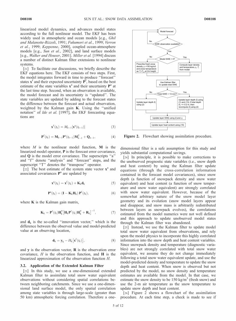
total snow water equivalent from observations, and relyupon the model physics to incorporate this highly correlatedinformation into the snow depth and heat content variables.Since snowpack density and temperature (diagnostic varia-bles) are not strongly correlated with total snow waterequivalent, we assume they do not change immediatelyfollowing a total snow water equivalent update, and use themodel-predicted density and temperature to update the snowdepth and heat content. When snow is observed but notpredicted by the model, no snow density and temperatureestimates are available from the model. In that case, weestimate the snow density to be 150 kg/m3 (fresh snow) anduse the 2-m air temperature as the snow temperature toupdate snow depth and heat content.[26] Figure 2 shows a flowchart of the assimilation

procedure. At each time step, a check is made to see if

Model forecast

SWE observation available?

Use Kalman filterto update total SWE

Total SWE > 13 mm?

Update layer SWE using Di and i

Update layer heat content using (15)

No

Yes

No Yes

No Yes

Model SWE > 0?

Update layer depth Diusing (2)

Prescribe fresh snow density i =150 kg/m3 and snow temperature as Ti=Tair at 2m height

Compute layer density and temperature i, Ti from model

Update layer depth Di using (1) and (13); if total depth DT <= 0.2 m, then recompute Di using (2)

ρ ρ

ρ

Figure 2. Flowchart showing assimilation procedure.


5 of 12

D08108

the observation SWE is available. If not, the model inte-grates one time step forward. If an observation is available,snow density and temperature in each layer are computed.Density ri in layer i is calculated as

ri ¼ rwWi= Diað Þ; ð9Þ

where rw = 1000 kg/m3 is the liquid water density and a isthe catchment fractional snow cover. The temperature Ti andfraction of ice fI,i are also diagnosed as

Ti ¼ 0

fI ;i ¼ �Hi= rwLf Wi

� �

8<: if Hi þ rw Lf Wi � 0 ð10Þ

and

Ti ¼ Hi þ fI ;i rw Lf Wi

� �= Cv;i Di a� �

fI ;i ¼ 1:0

8<: if Hi þ rw Lf Wi < 0;

ð11Þ

where Lf is the heat of fusion (J kg�1), and Cv,i is the heatcapacity of snow in layer i (J Kg�1 K�1). Cv,i is derivedfrom the heat capacity of ice as in the work of Verseghy[1991, equation (29)],

Cv;i ¼ Cv;ice ri=riceð Þ; ð12Þ

where Cv,ice = 2062 J Kg�1 K�1, and rice is the ice density,rice = 920 kg/m3.[27] The Kalman filter is then used to assimilate total

snow water equivalent WT (WT = W1 + W2 + W3). Thefractional snow cover a is updated as soon as WT has beenupdated (a = WT/Wc). If the three-layer mode is required(a = 1), then snow depths and layer thicknesses are updatedby the relationship

a r1D1 þ r2D2 þ r3D3ð Þ ¼ rwWT ; ð13Þ

using the appropriate substitution for Di from (1) or (2). Theoriginal snow density estimates and computed layerthicknesses are then used to compute the updated snowwater equivalent for each layer by

rwWi ¼ ariDi: ð14Þ

Likewise, the updated snow water equivalent and originaltemperature estimates are used to compute the heat contentfor each layer from

Hi ¼ TiCv;iDia� fI ;iLf Wi: ð15Þ

[28] If the relationship between WT and the thresholdvalue for full snow coverage Wc deems that the snow modelshould be in single-layer mode (WT < Wc), i.e., a < 1, thesingle-layer snow depth and heat content are computeddirectly from the updated total snow water equivalent WT

using (14) and (15).

4. Numerical Experiments

[29] We undertook a set of numerical ‘‘twin’’ experi-ments to develop the method to assimilate daily snow

water equivalent ‘‘observations’’ in North America. The‘‘observation’’ and evaluation data used in this study weregenerated from model output. The ‘‘twin’’ experiment isan important first step in the development of a dataassimilation system. These types of experiments allow usto determine the feasibility of the assimilation approachunder known conditions, namely the ‘‘truth.’’ This papershows how through the assimilation of snow water equiv-alent observations, the snow depth and heat content canalso be retrieved. By using a perfect model with perfectforcing and observations, we can clearly demonstrate howsnowpack state variables may be retrieved when the initialconditions are poorly known. Testing of this methodologyusing remotely sensed snow water equivalent observationsfrom both SMMR and SSM/I is the focus of a subsequentpaper.[30] The North American temporal and spatial snow-

pack evolution used here was generated by the catch-ment-based land surface model using the parameterspecification, forcing data and spin-up initial conditionsdescribed above. This simulation provided the ‘‘truth’’data for evaluation of our numerical experiments (hereaf-ter referred to as the ‘‘truth’’ run) and the ‘‘observation’’data for assimilation. To mimic the remotely sensedpassive microwave snow observations, the daily totalsnow water equivalent from the truth run was taken asour observation. The data used to evaluate the assimila-tion included snow water equivalent, snow depth, snowdensity, snow temperature, snow cover fraction, upwardshort- and long-wave radiation, as well as runoff andevapotranspiration from the truth run.[31] The truth run is contrasted with a degraded simula-

tion to illustrate snowpack initialization error impact onsnow state and atmospheric flux prediction, and the Kalmanfilter efficiency to correct poor snow state and atmosphericflux predictions. This simulation (hereafter referred to as the‘‘open loop’’ run) used the same model, parameters andatmospheric forcing as the truth run, but with degradedinitial conditions. The initial conditions are identical to thespin-up described above, with the exception that all snow-pack memory was erased on 1 January 1987 (i.e., it wasprescribed that no snow existed anywhere even though itwas in the middle of the snow season). We could have usedsnow climatology as the initial condition, but we choose thisextreme condition to illustrate the robustness of our assim-ilation scheme.[32] The extended Kalman filter assimilation experiment

(hereafter referred to as the ‘‘assimilation run’’) started withthe same degraded initial conditions as the open loop run,assimilating one total snow water equivalent observationper day. Note that availability of daily observations is not arequirement of the EKF; observations can be assimilated inEKF whenever they become available. To undertake theKalman filter assimilation, the linearized model function Mand knowledge of model and observation error statistics arerequired (see equations 4, 5, 6 and 7). We compute M usinga numerical approximation (forward finite difference) to thesnow prognostic Jacobian matrix. Since we only use theKalman filter to update total snow water equivalent, weonly need to forecast the total snow water equivalentvariance and not the covariances between all nine snowprognostic variables. Hence only the total snow water


6 of 12

D08108

equivalent Jacobian (now reduced to a scalar) needs to becalculated.[33] The error statistics, including model error covari-

ances Q, initial forecast error Pf (at time t = 0), andobservation error covariances R, are specified as following.We used an initial (20 mm)2 variance of model forecasterror variance Pf, a (10 mm)2 model error variance Q, and a(5 mm)2 total snow water equivalent observation errorvariance R. Note that these variances are only used in theEKF, while the ‘‘truth’’ and ‘‘observations’’ in the twinexperiments do not include additional added noises.

5. Results and Discussion

[34] Figures 3 and 4 compare snowpack forecasts fromthe open loop, assimilation and truth runs near the start of

January and middle of February, respectively. Figures 3aand 4a shows the impact of degraded snowpack initialcondition on snow forecast in the open loop run, ascompared to the truth run in Figures 3b and 4b. Incontrast, the assimilation scheme recovered the snow waterequivalent, snow temperature and snow fraction after onlyfive days of assimilation; see Figures 3c and 4c. Note thesnow depth in the assimilation run is overestimated ini-tially (Figure 3). That is because we depend on the modelto provide a snow density estimate. With the degradedinitial condition, the assimilation run starts with the default150 kg/m3 fresh snow density, which is lower than themature snowpack density. After one-and-half months,snow depth from the assimilation run has been recovered(Figure 4), since the density value becomes closer to thetrue value as the assimilation progresses. In contrast, snow

Figure 3. Snow simulation comparisons on 5 January 1987 over North America for snow waterequivalent (in mm, top row); snow depth (in mm, second row); average temperature (in �C, third row);and areal snow fraction (bottom row) from (a) open loop run (with degraded initial condition), (b) truthrun (using spin up initial condition), and (c) assimilation (with degraded initial condition and assimilationof daily total snow water equivalent observations).


7 of 12

D08108

density and depth in the open loop run never converged tothe true values.[35] The snow temperature and snow fraction variables

also maintain differences between the open loop and truthruns. While these are more subtle, they are not insignif-icant. It is not surprising that the assimilation is veryeffective in retrieving the snow water equivalent, since itis directly observed. However, the ability to also effec-tively retrieve the snow temperature and snow depth fromthis observation is significant. The snow temperaturediscussed here is the three-layer average, weighted byeach layer’s mass. It is a diagnostic variable that is afunction of snow water equivalent and heat content, andwhile strongly coupled to the air temperature, the effect isdampened by the snowpack’s thermal properties, throughboth the snow water equivalent and snow depth. As thesnow water equivalent and/or snowpack depth increases,it provides a greater insulation to the underlying snow. Inthe assimilation run, the snow temperature was recoveredvery rapidly due to the quick recovery of snow water

equivalent. In contrast, the open loop run produced a verylimited snow water equivalent amount, resulting in theforecast temperature being generally colder than the truetemperature, especially in northeastern Canada (Figures 3aand 4a).[36] As an example, Figure 5 shows the snowpack

evolution time series for two typical catchments. Theindividual snow water equivalent and snow depth timeseries over these two catchments clearly show how theassimilation run rapidly approached the true snow waterequivalent and gradually converged to the true snowdepth with time. This convergence of the snow depthwith time is a direct reflection of the snow densityconvergence, which occurs via the model physics as thesnowpack matures. In contrast, snow water equivalent,snow depth and snow density estimates in open loop runsstay below the true values throughout the three-monthperiod.[37] The assimilation snow forecast error location,

magnitude and persistence can be seen more clearly in

Figure 4. Same as Figure 3, except simulations are for 14 February 1987.


8 of 12

D08108

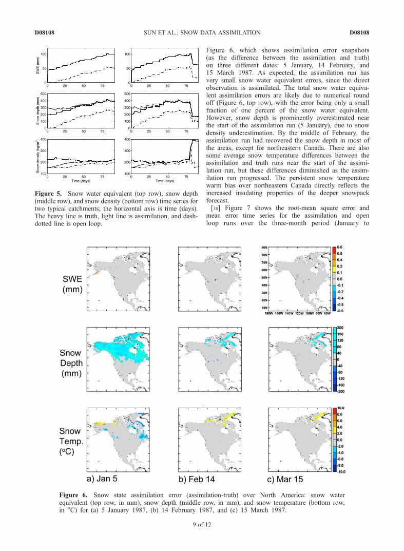
Figure 6, which shows assimilation error snapshots(as the difference between the assimilation and truth)on three different dates: 5 January, 14 February, and15 March 1987. As expected, the assimilation run hasvery small snow water equivalent errors, since the directobservation is assimilated. The total snow water equiva-lent assimilation errors are likely due to numerical roundoff (Figure 6, top row), with the error being only a smallfraction of one percent of the snow water equivalent.However, snow depth is prominently overestimated nearthe start of the assimilation run (5 January), due to snowdensity underestimation. By the middle of February, theassimilation run had recovered the snow depth in most ofthe areas, except for northeastern Canada. There are alsosome average snow temperature differences between theassimilation and truth runs near the start of the assimi-lation run, but these differences diminished as the assim-ilation run progressed. The persistent snow temperaturewarm bias over northeastern Canada directly reflects theincreased insulating properties of the deeper snowpackforecast.[38] Figure 7 shows the root-mean square error and

mean error time series for the assimilation and openloop runs over the three-month period (January to

Figure 5. Snow water equivalent (top row), snow depth(middle row), and snow density (bottom row) time series fortwo typical catchments; the horizontal axis is time (days).The heavy line is truth, light line is assimilation, and dash-dotted line is open loop.

Figure 6. Snow state assimilation error (assimilation-truth) over North America: snow waterequivalent (top row, in mm), snow depth (middle row, in mm), and snow temperature (bottom row,in �C) for (a) 5 January 1987, (b) 14 February 1987, and (c) 15 March 1987.


9 of 12

D08108

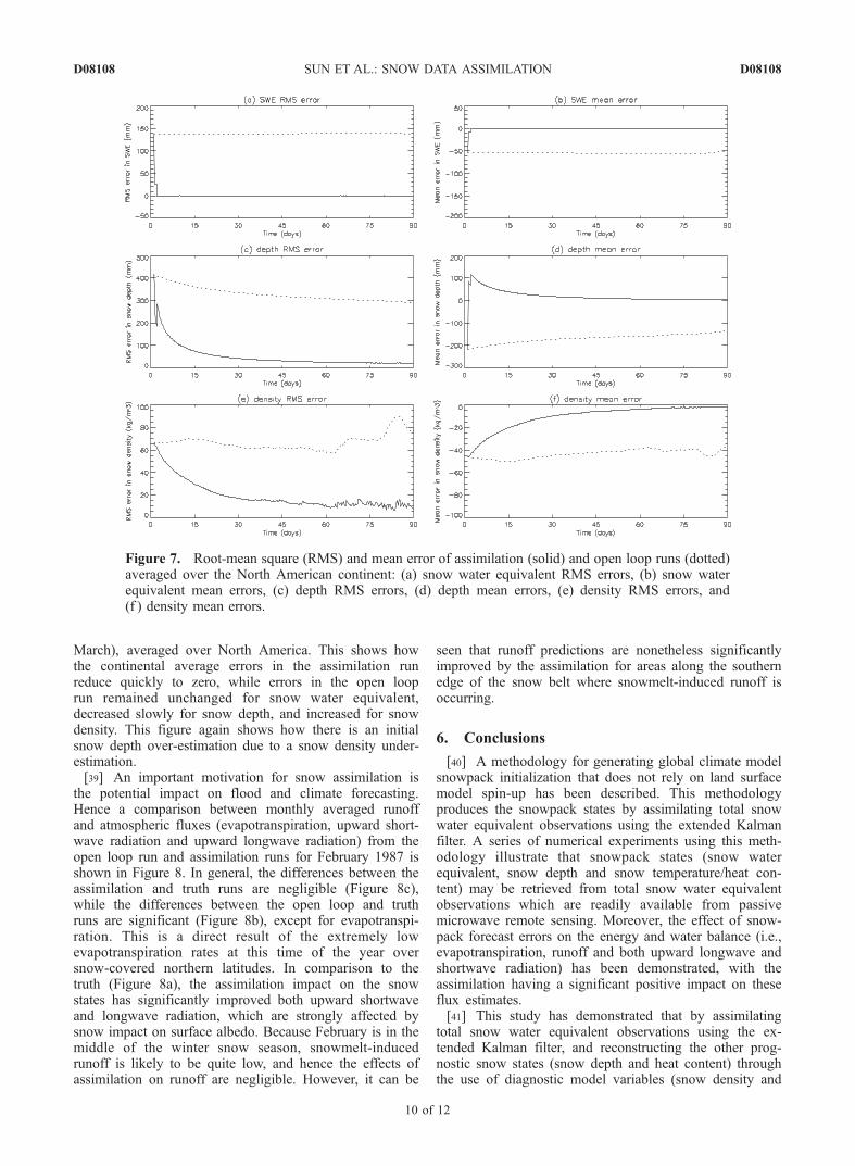
March), averaged over North America. This shows howthe continental average errors in the assimilation runreduce quickly to zero, while errors in the open looprun remained unchanged for snow water equivalent,decreased slowly for snow depth, and increased for snowdensity. This figure again shows how there is an initialsnow depth over-estimation due to a snow density under-estimation.[39] An important motivation for snow assimilation is

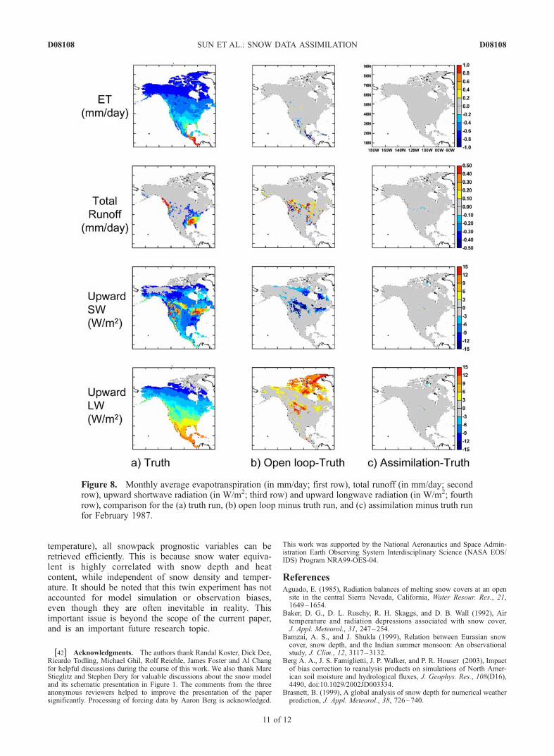
the potential impact on flood and climate forecasting.Hence a comparison between monthly averaged runoffand atmospheric fluxes (evapotranspiration, upward short-wave radiation and upward longwave radiation) from theopen loop run and assimilation runs for February 1987 isshown in Figure 8. In general, the differences between theassimilation and truth runs are negligible (Figure 8c),while the differences between the open loop and truthruns are significant (Figure 8b), except for evapotranspi-ration. This is a direct result of the extremely lowevapotranspiration rates at this time of the year oversnow-covered northern latitudes. In comparison to thetruth (Figure 8a), the assimilation impact on the snowstates has significantly improved both upward shortwaveand longwave radiation, which are strongly affected bysnow impact on surface albedo. Because February is in themiddle of the winter snow season, snowmelt-inducedrunoff is likely to be quite low, and hence the effects ofassimilation on runoff are negligible. However, it can be

seen that runoff predictions are nonetheless significantlyimproved by the assimilation for areas along the southernedge of the snow belt where snowmelt-induced runoff isoccurring.

6. Conclusions

[40] A methodology for generating global climate modelsnowpack initialization that does not rely on land surfacemodel spin-up has been described. This methodologyproduces the snowpack states by assimilating total snowwater equivalent observations using the extended Kalmanfilter. A series of numerical experiments using this meth-odology illustrate that snowpack states (snow waterequivalent, snow depth and snow temperature/heat con-tent) may be retrieved from total snow water equivalentobservations which are readily available from passivemicrowave remote sensing. Moreover, the effect of snow-pack forecast errors on the energy and water balance (i.e.,evapotranspiration, runoff and both upward longwave andshortwave radiation) has been demonstrated, with theassimilation having a significant positive impact on theseflux estimates.[41] This study has demonstrated that by assimilating

total snow water equivalent observations using the ex-tended Kalman filter, and reconstructing the other prog-nostic snow states (snow depth and heat content) throughthe use of diagnostic model variables (snow density and

Figure 7. Root-mean square (RMS) and mean error of assimilation (solid) and open loop runs (dotted)averaged over the North American continent: (a) snow water equivalent RMS errors, (b) snow waterequivalent mean errors, (c) depth RMS errors, (d) depth mean errors, (e) density RMS errors, and(f ) density mean errors.


10 of 12

D08108

temperature), all snowpack prognostic variables can beretrieved efficiently. This is because snow water equiva-lent is highly correlated with snow depth and heatcontent, while independent of snow density and temper-ature. It should be noted that this twin experiment has notaccounted for model simulation or observation biases,even though they are often inevitable in reality. Thisimportant issue is beyond the scope of the current paper,and is an important future research topic.

[42] Acknowledgments. The authors thank Randal Koster, Dick Dee,Ricardo Todling, Michael Ghil, Rolf Reichle, James Foster and Al Changfor helpful discussions during the course of this work. We also thank MarcStieglitz and Stephen Dery for valuable discussions about the snow modeland its schematic presentation in Figure 1. The comments from the threeanonymous reviewers helped to improve the presentation of the papersignificantly. Processing of forcing data by Aaron Berg is acknowledged.

This work was supported by the National Aeronautics and Space Admin-istration Earth Observing System Interdisciplinary Science (NASA EOS/IDS) Program NRA99-OES-04.

ReferencesAguado, E. (1985), Radiation balances of melting snow covers at an opensite in the central Sierra Nevada, California, Water Resour. Res., 21,1649–1654.

Baker, D. G., D. L. Ruschy, R. H. Skaggs, and D. B. Wall (1992), Airtemperature and radiation depressions associated with snow cover,J. Appl. Meteorol., 31, 247–254.

Bamzai, A. S., and J. Shukla (1999), Relation between Eurasian snowcover, snow depth, and the Indian summer monsoon: An observationalstudy, J. Clim., 12, 3117–3132.

Berg A. A., J. S. Famiglietti, J. P. Walker, and P. R. Houser (2003), Impactof bias correction to reanalysis products on simulations of North Amer-ican soil moisture and hydrological fluxes, J. Geophys. Res., 108(D16),4490, doi:10.1029/2002JD003334.

Brasnett, B. (1999), A global analysis of snow depth for numerical weatherprediction, J. Appl. Meteorol., 38, 726–740.

Figure 8. Monthly average evapotranspiration (in mm/day; first row), total runoff (in mm/day; secondrow), upward shortwave radiation (in W/m2; third row) and upward longwave radiation (in W/m2; fourthrow), comparison for the (a) truth run, (b) open loop minus truth run, and (c) assimilation minus truth runfor February 1987.


11 of 12

D08108

Brown, R., B. Brasnett, and D. Robinson (2001), Development of a griddedNorth American monthly snow depth and snow water equivalent datasetfor GCM validation, in Proceedings of the 58th Annual Meeting of East-ern Snow Conference, pp. 333–340, East. Snow Conf., Ottawa, Ont.

Brown, R., B. Brasnett, and D. Robinson (2003), Gridded North Americanmonthly snow depth and snow water equivalent for GCM evaluation,Atmos. Ocean, 41, 1–14.

Chang, A. T. C., J. L. Foster, and D. K. Hall (1987), Nimbus7 SMMRderived global snow cover parameters, Ann. Glaciol., 9, 39–44.

Cohen, J., and D. Entekhabi (1999), Eurasian snow cover variability andNorthern Hemisphere climate predictability, Geophys. Res. Lett., 26,345–348.

Dee, D. P., and A. M. da Silva (1998), Data assimilation in the presence offorecast bias, Q. J. R. Meteorol. Soc., 124, 269–295.

Dee, D. P., and R. Todling (2000), Data assimilation in the presence offorecast bias: The GEOS moisture analysis, Mon. Weather Rev., 128,3268–3282.

Dewey, K. F. (1977), Daily maximum and minimum temperature forecastsand the influence of snow cover, Mon. Weather Rev., 105, 1594–1597.

Ducharne, A., R. D. Koster, M. J. Suarez, M. Stieglitz, and P. Kumar(2000), A catchment-based approach to modeling land surface processesin a general circulation model: 2. Parameter estimation and modeldemonstration, J. Geophys. Res., 105, 24,823–24,838.

Foster, J. L., A. T. C. Chang, and D. K. Hall (1997), Comparison of snowmass estimates from a prototype passive microwave snow algorithm, arevised algorithm and a snow depth climatology, Remote Sens. Environ.,62, 132–142.

Fukumori, I., R. Raghunath, L.-L. Fu, and Y. Chao (1999), Assimilationof TOPEX/Poseidon altimeter data into a global ocean circulationmodel: How good are the results?, J. Geophys. Res., 104, 25,647–25,665.

Gelb, A. (1974), Optimal linear filtering, in Applied Optimal Estimation,edited by A. Gelb, pp. 102–155, MIT Press, Cambridge, Mass.

Ghil, M., and P. Malanotte-Rizzoli (1991), Data assimilation in meteorol-ogy and oceanography, Adv. Geophys., 33, 141–266.

Groisman, P. Y., T. R. Karl, and R. W. Knight (1994), Observed impact ofsnow cover on the heat balance and the rise of continental spring tem-peratures, Science, 263, 198–200.

Gutzler, P. Y., and R. D. Rosen (1995), Interannual variability of winter-time snow cover on the heat balance and the rise of continental springtemperatures, Science, 263, 198–200.

Hall, D. K. (1988), Assessment of polar climate change using satellitetechnology, Rev. Geophys., 26, 26–39.

Hall, D. K. (1998), Remote sensing of snow and ice using imaging radar, inManual of Remote Sensing, 3rd ed., pp. 677–703, Am. Soc. for Photo-gramm. and Remote Sens., Falls Church, Va.

Ide, K., P. Courtier, M. Ghil, and A. C. Lorenc (1997), Unified Notation fordata assimilation: Operational, sequential and variational, J. Meteorol.Soc. Jpn., 75, 181–189.

Johnson, R. H., G. S. Young, and J. J. Toth (1984), Mesoscale weathereffects of variable snow cover over northeast Colorado, Mon. WeatherRev., 112, 1141–1152.

Keppenne, C. L. (2000), Data assimilation into a primitive-equation modelwith a parallel ensemble Kalman filter, Mon. Weather Rev., 128, 1971–1981.

Koster, R. D., and M. J. Suarez (1995), Relative contributions of land andocean processes to precipitation variability, J. Geophys Res., 100,13,775–13,790.

Koster, R. D., M. J. Suarez, A. Ducharne, M. Stieglitz, and P. Kumar(2000), A catchment-based approach to modeling land surface processesin a general circulation model: 1. Model structure, J. Geophys. Res., 105,24,809–24,822.

Liston, G. E., R. A. Pielke Sr., and E. M. Greene (1999), Improving first-order snow-related deficiencies in a regional climate model, J. Geophys.Res., 104, 19,559–19,567.

Lo, F., and M. P. Clark (2002), Relationships between spring snow massand summer precipitation in the southwestern United States associatedwith the North American monsoon system, J. Clim., 15, 1378–1385.

Lynch-Stieglitz, M. (1994), The development and validation of a simplesnow model for the GISS GCM, J. Clim., 7, 1842–1855.

Miller, R. N., M. Ghil, and F. Gauthiez (1994), Advanced data assimila-tion in strongly nonlinear dynamical systems, J. Atmos. Sci., 51, 1037–1056.

Mitchell, K., et al. (2002), Reducing near-surface cool/moist biases oversnowpack and early spring wet soils in NCEP ETA model forecasts vialand surface model upgrades, in Proceedings of the 16th Conference onHydrology and 13th Symposium on Global Change and Climate Varia-tions, pp. J1–J6, Am. Meteorol. Soc., Boston, Mass.

Namias, J. (1985), Some empirical evidence for the influence of snow coveron temperature and precipitation, Mon. Weather Rev., 113, 1542–1553.

Robinson, D. A. (2002), Developing a blended continental snow coverdataset, in Proceedings of the 16th Conference on Probability and Sta-tistics in the Atmospheric Sciences and the Symposium on Observations,Data Assimilation, and Probabilistic Prediction, pp. 87 – 88, Am.Meteorol. Soc., Boston, Mass.

Robinson, D. A., and G. Kukla (1985), Maximum surface albedo of sea-sonally snow-covered lands in the Northern Hemisphere, J. Clim. Appl.Meteorol., 24, 402–411.

Robinson, D. A., K. F. Dewey, and R. R. Heim (1993), Global snow covermonitoring: An update, Bull. Am. Meteorol. Soc., 74, 1689–1696.

Rodell, M., et al. (2004), The Global Land Data Assimilation System, Bull.Am. Meteorol. Soc., 85(3), 381–394.

Sellers, P. J., J. Collatz, and F. G. Hall (1996), The ISLSCP Initiative Iglobal data sets: Surface boundary conditions and atmospheric for-cings for land-atmosphere studies, Bull. Am. Meteorol. Soc., 77,1987–2005.

Stieglitz, M., A. Ducharne, R. Koster, and M. Suarez (2001), The impact ofdetailed snow physics on the simulation of snow cover and subsurfacethermodynamics at continental scales, J. Hydrometeorol., 2, 228–242.

Sud, Y. C., and D. M. Mocko (1999), New Snow-physics to complementSSiB. Part I: Design and evaluation with ISLSCP Initiative I datasets,J. Meteorol. Soc. Jpn., 77(1B), 335–348.

Sun, C., Z. Hao, M. Ghil, and J. D. Neelin (2002), Data assimilation for acoupled ocean-atmosphere model. Part I: Sequential state estimation,Mon. Weather Rev., 130, 1073–1099.

Verron, J., L. Gourdeau, D. T. Pham, R. Murtugudde, and A. J. Busalacchi(1999), An extended Kalman filter to assimilate satellite altimeter datainto a nonlinear numerical model of the tropical Pacific Ocean: Methodand validation, J. Geophys. Res., 104, 5441–5458.

Verseghy, D. L. (1991), CLASS—A Canadian land surface scheme forGCMS. I: Soil model, Int. J. Climatol., 11, 111–133.

Walker, J. P., and P. R. Houser (2001), A methodology for initializing soilmoisture in a global climate model: Assimilation of near-surface soilmoisture observations, J. Geophys. Res., 106, 11,761–11,774.

��P. R. Houser, Hydrological Sciences Branch, Laboratory for Hydro-

spheric Processes, NASA Goddard Space Flight Center, Greenbelt, MD20771, USA.C. Sun, Code 900.3, Global Modeling and Assimilation Office, NASA

Goddard Space Flight Center, Greenbelt, MD 20771, USA. ([email protected])J. P. Walker, Department of Civil and Environmental Engineering,

University of Melbourne, Parkville, Victoria 3010, Australia.


12 of 12

D08108

a methodology for snow data assimilation in a land surface ... · a methodology for snow data...

Documents