a method for structure analysis of eeg data -application...

IJCSNS International Journal of Computer Science and Network Security, VOL.9 No.9, September 2009

70

Manuscript received November 5, 2008

Manuscript revised November 20, 2008

A Method for Structure Analysis of EEG Data

-Application to ANOVA in Vegetable Ingestion-

Takashi Ajiro†, Akiko Yamanouchi††, Koichiro Shimomura†, Hirobumi Yamamoto† and Kenichi Kamijo†

†Plant Regulation Research Center, Toyo University, 1-1-1 Izumino, Itakra, Gunma, 374-0193, Japan ††Izu Oceanics Research Institute, 3-12-23 Nishiochiai, Shinjuku, Tokyo, 161-0031, Japan

Summary Electroencephalogram (EEG) data, which consist of weak voltage values of the brain measured over time, are recorded by EEG measuring instruments (Brain Builder Unit in this study). These data are captured in real time and written to a file in CSV (Comma Separated Values) format. By applying several processes using the data, we extract the crossed data and conduct an analysis of variance (ANOVA), and we assess the significance of the influence of the measuring object on the EEG of a human examinee. First, we captured EEG patterns of examinees ingesting the vegetable komatsuna and then conducted the ANOVA to determine whether the growing condition of the vegetable affects the EEG pattern of the examinee. However, much manual work and time are needed to convert the EEG to the data for displaying graph on Microsoft Excel 2003, and analysing it by ANOVA software. Therefore, we propose an automation algorithm for converting the captured data from the EEG measuring device, and we develop (implement) a program based on this algorithm. Specifically, the automation algorithm combines these manual processes to make the two kinds of data needed for ANOVA and for Excel graphs, and the C++ program generates the actual data. Key words: ANOVA, SOC, EEG, vegetable ingestion, komatsuna, algorithm, program implementation,

1. Introduction

An electroencephalogram (EEG), which records brain activity, is commonly used in many clinical and research areas because it is not invasive and fatiguing for the examinee and the measurement instruments are relatively low in cost. Since EEG responses indicate fluctuations in the electrical activity of the human brain (in other words, psychological influences), there have been many studies that measure the effects of sensory inputs, such as hearing, smell, vision and taste, on EEG activity [1-6]. Additional applications using EEG are now being considered, including research on human interfaces [7]. We measured EEG activity with a simplified EEG measurement device named the "Brain Builder Unit" [8] of a examinee eating a

piece of vegetable called komatsuna and statistically assessed the significance of the data by an analysis of variance (ANOVA). Similar research projects have collected EEG data of examinees drinking alcohol and milk [9-10]. However, our research approach has two distinct differences: first, we focused on the EEG fluctuations due to the differences of fertilizers for cultivating vegetables. In particular, we researched the relaxation effects on (Japanese) humans ingesting komatsuna grown using different fertilizers. Second, we supplemented our results with ANOVA, a statistical approach rarely used in this domain. Because ANOVA indicates statistically significant differences, verification of the results is more precise than that using general non-statistical methods.

Komatsuna cultivation have existed since the Edo Period in Komatsugawa, Edogawa-ku, Tokyo-to, Japan (current geographic name). The komatsuna vegetable was allegedly named as a tribute to the early cultivation prefectures, although now this vegetable is cultivated in Tokyo as well as neighbouring prefectures. An example of a komatsuna is shown in Fig. 1. In our experiments, the examinees were requested to eat every part except that directly under the stem. Previously, we researched the vegetable's benefits, such as antioxidative activity and vitamin content. It is known that the same kind of vegetable tastes differently depending on the use of organic fertilizer or chemical fertilizer. By using a flavor recognition machine (TS-5000Z, Intelligent Sensor Technology Inc.), we found that an astringent taste and a bitter taste are indices to distinguish the taste of komatsuna's [11]. The machine, shown in Fig. 2, is located at the Plant Regulation Research Center, Toyo University. We analysed the EEG fluctuations depending on different komatsuna tastes. The results presented in this paper also indicate the differences in statistical significance by the analysis of variance.

The processes to analyze and graph EEG data using Excel 2003 software require many hours and much human interaction. By automating these processes, many analysis


71

costs (e.g., time) and human errors can be reduced. With this background, we devised two algorithms to process EEG data (in ".fft" files) obtained by the simple EEG measurement instrument "Brain Builder Unit" and developed programs utilizing these algorithms. One algorithm generates data files in the CSV (Comma Separated Values, in ".csv" files) format and includes data for ANOVA, which is carried out with statistical calculation software called JUSE-QCAS Version 7 [12]. The another algorithm takes the data generated by the first algorithm and generates data for graphing in Excel 2003. In this paper, we explain the details of these algorithms and the program we developed to integrate and execute the algorithms.

Fig. 1 Komatsuna (green vegetable)

Fig. 2 Flavor recognition machine TS-5000Z

2. Preliminary Experiment on Komatsuna Ingestion

2.1 Equipment for the Measurements and Analysis

1) EEG measurement instrument: As introduced in the previous section, we used a simple EEG measurement device called the "Brain Builder Unit" for

EEG measurement [9]. A photograph of this device, including the electrodes, is shown in Fig. 3. The two electrodes of the headband contact the skin on the forehead of a human face, and the other electrode is an electric wire that clips onto the left ear lobe. The measurement device is connected to a PC with the Windows operating system (more recent than Win98). EEG measurement software called Mind Sensor II controls the Brain Builder Unit [9]. A photograph of the Mind Sensor II is shown in Fig. 4. The software communicates to the measurement device by a serial port and captures and writes out the EEG data. The system measures EEG data of the right and left brain separately, and the measured data series is written to an ".fft" file that has an internal CSV format. Figure 4 shows the data visualization function of the software, which displays a real-time electric pattern during the EEG capturing process. These patterns are of two kinds: one is the raw voltage fluctuation (unit: uV), and the other is the spectrum that indicates each power of frequency by Fast Fourier Transformation (FFT).

Fig. 3 The Brain Builder Unit with three electrodes

Fig. 4 Display of Mind Sensor II (in Japanese)


72

2) Definitions of EEG frequency groups: In general, the categorized spectrum defined in an EEG frequency grouping is used in the EEG analysis instead of the raw electrical fluctuation or its spectrum, even though definitions of EEG frequency groupings vary according to the researcher. For example, some EEG books [13-14] introduce definitions for EEG frequency groupings. We used the definitions in the manual of the Mind Sensor II software, since the definitions are confined to our research and are valid definitions. The EEG frequency groupings defined for the experiment are as follows. δ wave -------- 1 ~ 4 Hz (deep sleep) θ wave -------- 5 ~ 7 Hz (light sleep, meditation) α wave -------- 8 ~ 15 Hz (relaxing, creativity uplifting) slow α wave --- 8 ~ 9 Hz mid α wave --- 10 ~ 12 Hz fast α wave --- 13 ~ 15 Hz β wave -------- 16 ~ 24 Hz (attention, concentration)

The δ wave-group (hereafter, a wave-group is called

a "wave") appears in deep sleep, but we cannot use this wave since the EEG measurement device mixes electrical noise. We also cannot use the θ wave since the examinees are awake. The area of the α wave is separated into three groupings, since these frequencies are the most important for examining relaxation effects. In addition, fluctuations of these frequencies are active only in awake humans. The β wave is a wave that appears in the attention state, and we use it in comparison with the α-type waves. Although the general boundary of the β wave is considered to be 40 Hz, our definition is 24 Hz due to the limitation of the measurement device.

3) ANOVA Software for analysis variance: For

the ANOVA calculations, captured EEG data in the ".fft" file is processed and input into software called JUSE-QCAS Version 7 [10]. This software supports many statistical operations, including the ANOVA function. Figure 5 shows a snapshot of the data-editing mode of this software. In the editing mode, the user can input data to cells that accept integer values, real values, and characters as text labels. The system recognizes the columns of these cells as two kinds of variables: "quality variables" and "quantity variables". The quality variables include the "levels" of "factors", and the quantity variables include the analysis data. In Fig. 5, C3 ~ C5 are quantity columns and N6 ~ N7 are quality columns. The system analyzes quality values (measurement data) according to the factors and allocations of the quantity values (levels of factors). As the result, the software generate a tables of ANOVA data (called ANOVA table).

Fig. 5 Display of JUSE-QCAS Version 7 (in Japanese)

2.2 Preparing for the Experiments

The experimental sequence was carried out as follows: "Hearing the BGM (before phase: 60 sec) → Eating pieces of komatsuna (during phase: 60 sec) → Hearing the BGM (after phase: 60 sec)". The meaning of BGM hearing phase is to stabilize the examinee's psychological state. The experimental order of examinees is "male of pair 1, female of pair 1, male of pair 2, female of pair 2". The "examinees" and "executors" are not given any information about the kinds of komatsuna (double-blind experiment). More details of our experimental conditions are as follows.

Examinees put on the EEG measurement device (Brain Builder Unit) and a noise cancelling headphone connected to a CD player. All experiments are conducted in a partitioned space, which includes a table for eating the samples. The examinees must sit down and be silent. Examinees eat (manducate and drink) a piece of komatsuna in the "during" stage. They must eat a piece after 30 seconds. "Sekai no shasou kara" (in English: "From Train Windows in the World") is used as the music intended to cancel the environmental noise along with the noise cancelling by the headphones. The examinee must scoop and eat meals with a spoon, since spoon-feeding by another person is a rare action that may generate an invalid EEG measurement result due to the psychological effect. All komatsunas for these experiments are boiled in tap water and then squeezed until they are 90% of the initial weight.

Our experimental environment and measuring

equipment are shown in Fig. 6. The experimental room is partitioned by the tent, shown in the top left photo, and the inside tent area is shown in the top right photo. Komatsuna pieces for the experiments are put in large, covered petri dishes (approximately 15 cm) and placed on the table.


73

Thus, examinees need to lift the cover of the petri dish when they eat the komatsuna. A spoon is also put on the table and rests on the side of the petri dish.

The bottom photo in Fig. 6 shows our experimental equipment. The Brain Builder Unit is connected to the serial port of the black computer, and the connected monitor displays Mind Sensor II. The lotion is used for the Brain Builder's electrodes, since these must contact the skin of the examinee. The CD Player plays music before starting the first experiment, and the executors need only to push the start button to play the music. The headphone outputs the music, cancelling environment noise (especially low pitch sound).

Fig. 6 Experimental equipment for the EEG measurements

2.3 Preliminary Experiments and the Results

We conducted preliminary experiments two times to inspect the EEG fluctuations of humans eating pieces of komatsuna. These measurement data were processed by the EEG calculation method previously used by our research group. The method is described as follows.

(1) Separate all values to values according to each brain.

(2) Calculate each the average value of each phase (before, during, after), side of brain, frequency.

(3) Select the maximum value of each phase and side of brain from each EEG frequency group (there are slow α, mid α, fast α, and β)

A simple explanation of these operation sequences is to average the values per phase and side of brain, and to select the maximum value from each of these results. For example, the value of mid α wave (phase: before, brain: left) is the maximum value of the averages of each value (power) of 10, 11 and 12 Hz. This method assumes the maximum value of averages in each wave group is the central value (in other words, primary value).

We generated data patterns to use in the analyses by JUSE-QCAS and to make fluctuation graphs by the calculation method. The format of these data is optimised for JUSE-QCAS, and graph data were generated by gathering the needed data and calculating their average. Specifically, we made tables that consist of "3 column (phases) x 2 rows (kinds)" in Excel sheets. There are two kinds of tables and graphs: immediate tables (graphs) and relative tables. The former are tables using immediate data, and the latter are tables using relative fluctuation data, when the value is "before," which is 0 (unit: μV).

1) Preliminary Experiment 1 (Ex. 1): Examinee pairs consist of a male and a female, and two pairs (four people) were tested. They ate two kinds of komatsunas that had been cultivated by either organic or chemical fertilizer. Thus, we obtained 2 x 4 = 8 data for the ".fft" file, as measured by the Brain Builder Unit. The results are shown as relative value graphs in Fig. 7. In this paper, we do not show immediate graphs, since they are not as helpful and the necessity of these graphs is only intermediate values for generating relative graphs.

We conclude that the results indicate the usefulness of continuing this research, since the two kinds of graphs show differences, although the measurement condition is the same.

EEG Fluctuation (slow α)

-3

-2

-1

0

1

2

3

4

5

6

7

before during after

Phase

Re

lati

ve

Volt

age

(μ

V)

organic

chemical

EEG Fluctuation (mid α)

-3

-2

-1

0

1

2

3

4

5

before during after

Phase

Re

lati

ve

Vo

ltage (

μV

)

organic

chemical


74

EEG Fluctuation (fast α)

-3

-2

-1

0

1

2

3

4

5

before during after

Phase

Re

lati

ve

Vo

ltage

(μ

V)

organic

chemical

EEG Fluctuation (β)

-3

-2

-1

0

1

2

3

4

5

before during after

Phase

Rela

tive V

olt

age

(μ

V)

organic

chemical

Fig. 7 The fluctuation graph (relative values) for Ex. 1

2) Preliminary Experiment 2 (Ex. 2): As in Ex. 1,

examinee pairs consist of a male and a female, and two pairs (four people) were tested. They ate a total of six sets of komatsunas that had been cultivated by organic, chemical, and organic + chemical fertilizers. Two kinds of the same komatsunas had been cultivated in two different farm fields. Thus, we obtained 6 x 2 = 24 ".fft" data by the Brain Builder Unit. The results are shown as relative value graphs in Fig. 8. Data of the different farm fields were averaged as one value, and this average was set as a point of the fluctuation graphs. The results indicate each wave fluctuation is different in the "during" phase. Considering the results of Ex. 1 and Ex. 2, examinees eating pieces of komatsuna grown with organic fertilizer have β waves in the "after" phase that are lower than in the "before" phase. Again, we conclude that the results indicate the usefulness of continuing this research, since the three graphs show differences, although the measurement condition was the same. However, we need to consider the points of inconstant fluctuation per wave.

EEG Fluctuation (slow α)

-2

0

2

4

6

8

10

before during after

Phase

Re

lati

ve

Vo

ltage

(μ

V)

organic

chemicalorg+che

EEG Fluctuation (mid α)

0

0.5

1

1.5

2

2.5

3

3.5

4

before during after

Phase

Re

lati

ve

Vo

ltage

(μ

V)

organic

chemicalorg+che

EEG Fluctuation (fast α)

-1

0

1

2

3

4

5

6

7

8

9

before during afterPhase

Re

lati

ve V

olt

age

(μ

V)

organic

chemicalorg+che

EEG Fluctuation (β)

-2

0

2

4

6

8

10

before during after

Phase

Re

lati

ve

Vo

ltage

(μ

V)

organic

chemicalorg+che

Fig. 8 The fluctuation graph (relative values) for Ex. 2

3. Analysis of Variance (ANOVA)

3.1 Basic Concept of the ANOVA

The ANOVA statistical analysis method is based on the dependencies of factors related to the movement of the measurement values. In this method, independent factors are called "main effects," and factors made by mixing independent factors are called "interactions." The main factors are denoted as "A", "B", "C" and the interactions are denoted as "A x B", "B x C", "A x C". The calculation results are called "p-values" (probability values) by a function of this method called an "assay." The result of the assay is represented by "**" if the p-value is less than 0.01, or by "*" if the p-value is less than 0.05. The p-value indicates the reliability of the significance. As an example, a p-value of 0.5 indicates statistical singular values of 5% that are included in the enormous measured value.


75

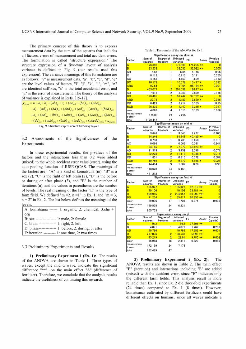
The primary concept of this theory is to express measurement data by the sum of the squares that includes all factors, errors of measurement and total accident errors. The formulation is called "structure expression." The structure expression of a five-way layout of analysis variance is defined in Fig. 9 (our results used this expression). The variance meanings of this formulation are as follows: "y" is measurement data, "a", "b", "c", "d", "e" are the level values of factors, "i", "j", "k", "l", "m", "n" are identical suffixes, "ε" is the total accidental error, and "μ" is the error of measurement. The theory of the analysis of variance is explained in Refs. [15-17].

Fig. 9 Structure expression of five-way layout

3.2 Assessments of the Significances of the Experiments

In these experimental results, the p-values of the factors and the interactions less than 0.2 were added (mixed) to the whole accident error value (error), using the auto pooling function of JUSE-QCAS. The meanings of the factors are : "A" is a kind of komatsuna (m), "B" is a sex (2), "C" is the right or left brain (2), "D" is the before or during or after phase (3), and "E" is the number of iterations (n), and the values in parentheses are the number of levels. The real meaning of the factor "E" is the type of farm field. We defined "m =2, n =1" in Ex. 1, and "m = 3, n = 2" in Ex. 2. The list below defines the meanings of the levels.

A: komatsuna ------ 1: organic, 2: chemical, 3:che + org B: sex --------------- 1: male, 2: female C: brain ------------- 1: right, 2: left D: phase------------- 1: before, 2: during, 3: after E: iteration --------- 1: one time, 2: two times

3.3 Preliminary Experiments and Results

1) Preliminary Experiment 1 (Ex. 1): The results of the ANOVA are shown in Table 1. Three types of waves, except the mid α wave, indicate the significant difference "**". on the main effect "A" (difference of fertilizer). Therefore, we conclude that the analysis results indicate the usefulness of continuing this research.

Table 1: The results of the ANOVA for Ex 1

FactorSum ofsquares

Degree offreedom

Unbiasedvariance

F0 AssayP-value(upside)

A 176.898 1 176.898 174.205 ** 0B 33.533 1 33.533 33.022 ** 0.005AB 6.85 1 6.85 6.746 0.06C 0.113 1 0.113 0.111 0.755AC 4.153 1 4.153 4.09 0.113BC 10.578 1 10.578 10.417 * 0.032ABC 97.64 1 97.64 96.154 ** 0.001D 403.077 2 201.539 198.47 ** 0AD 7.918 2 3.959 3.899 0.115BD 198.485 2 99.242 97.732 ** 0ABD 27.78 2 13.89 13.679 * 0.016CD 6.429 2 3.214 3.165 0.15BCD 26.839 2 13.42 13.215 * 0.017error 4.062 4 1.015 0.139 0.966measurement error

175.09 24 7.295

total 1179.447 47

Significance assay on slow α

FactorSum ofsquares

Degree offreedom

Unbiasedvariance


A 3.646 1 3.646 2.277 0.166B 64.846 1 64.846 40.489 ** 0C 0.733 1 0.733 0.458 0.516AC 0.066 1 0.066 0.041 0.844D 154.145 2 77.072 48.123 ** 0AD 11.519 2 5.759 3.596 0.071BD 22.225 2 11.113 6.938 * 0.015CD 1.831 2 0.916 0.572 0.584ACD 19.759 2 9.879 6.168 * 0.021error 14.414 9 1.602 0.26 0.98measurement error

148.028 24 6.168

total 441.212 47

Significance assay on mid α

FactorSum ofsquares

Degree offreedom

Unbiasedvariance


A 105.927 1 105.927 62.019 ** 0B 40.106 1 40.106 23.481 ** 0D 409.915 2 204.957 119.999 ** 0BD 71.234 2 35.617 20.853 ** 0error 29.036 17 1.708 0.274 0.996measurement error

149.535 24 6.231

total 805.753 47

Significance assay on fast α

FactorSum ofsquares

Degree offreedom

Unbiasedvariance


A 86.2 1 86.2 37.308 ** 0B 4.071 1 4.071 1.762 0.203AB 40.786 1 40.786 17.652 ** 0.001D 277.076 2 138.538 59.96 ** 0BD 45.219 2 22.61 9.786 ** 0.002error 36.968 16 2.311 0.322 0.989measurement error

172.169 24 7.174

total 662.489 47

Significance assay on β

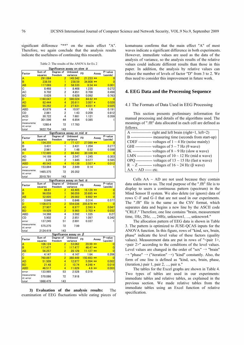
2) Preliminary Experiment 2 (Ex. 2): The

ANOVA results are shown in Table 2. The main effect "E" (iteration) and interactions including "E" are added (mixed) with the accident error, since "E" indicates only the different farm fields. This analysis result is more reliable than Ex. 1, since Ex. 2 did three-fold experiments (24 times) compared to Ex. 1 (8 times). However, komatsunas cultivated by different fertilizers could have different effects on humans, since all waves indicate a


76

significant difference "**" on the main effect "A". Therefore, we again conclude that the analysis results indicate the usefulness of continuing this research.

Table 2: The results of the ANOVA for Ex 2

FactorSum ofsquares

Degree offreedom

Unbiasedvariance


A 291.084 2 145.542 21.233 ** 0B 238.59 1 238.59 34.808 ** 0AB 117.069 2 58.535 8.54 ** 0.001C 8.468 1 8.468 1.235 0.272AC 9.702 2 4.851 0.708 0.498BC 0.628 1 0.628 0.092 0.763D 1160.047 2 580.024 84.62 ** 0AD 82.444 4 20.611 3.007 * 0.028BD 55.262 2 27.631 4.031 * 0.025ABD 43.879 4 10.97 1.6 0.191CD 2.861 2 1.43 0.209 0.812ACD 30.722 4 7.681 1.121 0.359error 301.596 44 6.854 0.385 1measurement error

1280.4 72 17.783

total 3622.754 143

Significance assay on slow α

FactorSum ofsquares

Degree offreedom

Unbiasedvariance


A 154.255 2 77.127 27.069 ** 0B 3.431 1 3.431 1.204 0.277AB 2.961 2 1.48 0.52 0.598D 172.885 2 86.442 30.338 ** 0AD 14.189 4 3.547 1.245 0.303BD 3.29 2 1.645 0.577 0.565ABD 40.543 4 10.136 3.557 * 0.012error 153.864 54 2.849 0.14 1measurement error

1465.375 72 20.352

total 2010.791 143

Significance assay on mid α

FactorSum ofsquares

Degree offreedom

Unbiasedvariance


A 86.81 2 43.405 16.129 ** 0B 96.059 1 96.059 35.695 ** 0AB 52.005 2 26.002 9.662 ** 0C 0.846 1 0.846 0.314 0.577D 1108.073 2 554.036 205.879 ** 0AD 27.907 4 6.977 2.593 * 0.047BD 19.929 2 9.965 3.703 * 0.032ABD 14.368 4 3.592 1.335 0.27CD 5.902 2 2.951 1.097 0.342error 137.245 51 2.691 0.337 1measurement error

575.275 72 7.99

total 2124.419 143

Significance assay on fast α

FactorSum ofsquares

Degree offreedom

Unbiasedvariance


A 106.124 2 53.062 20.99 ** 0B 117.477 1 117.477 46.47 ** 0AB 56.257 2 28.129 11.127 ** 0C 4.147 1 4.147 1.64 0.206D 760.897 2 380.449 150.493 ** 0AD 51.509 4 12.877 5.094 ** 0.002BD 21.48 2 10.74 4.248 * 0.019ABD 46.517 4 11.629 4.6 ** 0.003error 133.985 53 2.528 0.319 1measurement error

570.086 72 7.918

total 1868.479 143

Significance assay on β

3) Evaluation of the analysis results: The

examination of EEG fluctuations while eating pieces of

komatsuna confirms that the main effect "A" of most waves indicate a significant difference in both experiments. However, immediate values are used as the data of the analysis of variance, so the analysis results of the relative values could indicate different results than those in this paper. In addition, the analysis by relative values can reduce the number of levels of factor "D" from 3 to 2. We thus need to consider this improvement in future work.

4. EEG Data and the Processing Sequence

4.1 The Formats of Data Used in EEG Processing

This section presents preliminary information for manual processing and details of the algorithms used. The meanings of ".fft" data allocated in each cell are defined as follows. A --------------- right and left brain (right=1, left=2) B ---------------- measuring time (seconds from start-up)CDEF ---------- voltages of 1 ~ 4 Hz (noise mainly) GHI ------------ voltages of 5 ~ 7 Hz (θ wave) JK -------------- voltages of 8 ~ 9 Hz (slow α wave) LMN ----------- voltages of 10 ~ 12 Hz (mid α wave) OPQ ------------ voltages of 13 ~ 15 Hz (fast α wave) R ~ Z ---------- voltages of 16 ~ 24 Hz (β wave) AA ~ AD ----- etc.

Cells AA ~ AD are not used because they contain

data unknown to us. The real purpose of the ".fft" file is to display to users a continuous pattern (spectrum) in the Mind Sensor II system. We also delete (or ignore) data of rows C~F and G~I that are not used in our experiments. The ".fft" file is the same as the CSV format, which separates data and begins a new line by the ASCII code "CRLF." Therefore, one line contains "brain, measurement time, 1Hz, 2Hz, ..., 24Hz, unknown1, ..., unknown4."

The allocation pattern of EEG data is shown in Table 3. The pattern is optimized to JUSE-QCAS inputs for the ANOVA function. In this figure, rows of "kind, sex, brain, phase" indicate the level value of these factors (quality values). Measurement data are put in rows of "<pair 1>, <pair 2>" according to the conditions of the level values. Level values are changed in the order of "sex" → "brain" → "phase" → ("iteration" →) "kind" constantly. Also, the form of one line is defined as "kind, sex, brain, phase, (iteration,) pair 1, pair 2, ..., pair n."

The tables for the Excel graphs are shown in Table 4. Two types of tables are used in our experiments: immediate tables and relative tables, as explained in the previous section. We made relative tables from the immediate tables using an Excel function of relative specification.


77

Table 3: The allocation pattern of EEG data to ANOVA

Table 4: Tables for Excel graphs using immediate values (left) and relative values (right)

4.2 Manual Processing on the Excel 2003 System

Here, we summarize the manual algorithm. Small-number operations execute earlier than large-number operations, and the lines execute in consecutive order. Closely indented operations mean an iteration (loop) or condition (branch) structure. Details of the full manual algorithm on the Excel 2003 system are presented in the following.

(1) Prepare the ".fft" data file for examinee number "n" in pair "m", and then change the file extension ".fft" to ".csv" and open it by Excel 2003.

(2) Sort the all data ascending by values of brains (right =1, left = 2).

(3) Insert about 2 ~ 3 rows into each part between "before" and "during", and between "during" and "after".

(4) Put on the averaged values (calculated by AVERAGE function) to each J ~ Z column under each part of "before", "during" and "after".

(5) Put on the maximum value by the averaged values (calculated by MAX function) to the part under the last row (put on the averaged value) of each column JK LMN OPQ R ~ Z.

(6) Assemble the maximum value of the averaged values onto an area of far empty cells under the data part.

(7) Save the current editing data by the same name (this extension must be ".xls").

(8) If there are not finished examinee's data (if ".fft" files without corresponding ".xls" files exist), then go to (1) to process other examinee's data.

(9) Create a new ".xls" file and it can be a freedom name, and define imaginary variable "x" and set it to 1.

(10) Add a sheet and name it to the name corresponding to

"x", and set it to current workspace1٭. But, do not add it if enough empty sheets exist.

(11) In the sheet, make the data table formatted in "Komatsuna, Male or female, Right or left brain, Phase" for giving to JUSE-QCAS2٭. The table includes all assembled data of files made in (7), and allocates them according to the defined pattern.

(12) Put on the table formatted in "Examinee pair 1, Examinee Pair 2" on the right neighbour cells to it3٭.

(13) Put on the table for Excel graphs, operating averages from data of same phases and kinds (the table of immediate values). And, put on the table by relative values from "before", using the immediate values.

(14) If "x" < 4, then 1 is added to "x" and go to (10). = Wave names corresponding to "x" is: 1 = "slow α", 2 1٭

"mid α", 3 = "fast α", 4 = "β". In Ex. 2, The table is formatted in "Komatsuna, Male and 2٭

female, Right or left brain, Phase, Iteration". Two examinee data on same column must be same sex to 3٭

correspond to the level value of "Male and female".

The visual flow of the manual algorithm is shown in

Fig. 10. The numbers corresponding to an operation are represented in a side of the one. For instance, processes (4) and (5) are placed on a side of the center image (light violet and pink cells). Thick arrows are used normal processes execution, and slim arrows are used only for loops. As the exception, (9) is represented by gray text as a one-time execution without looping.

Fig. 10 Visual flow of the manual processing method


78

5. Automation of EEG Data Processing

5.1 Overview of Our Automation Algorithm

As a method for reducing the complicated manual processing, we devised an automation algorithm for computer processing. The algorithm differs greatly from the manual one, since the automatic processes do not require the Excel system. Instead, the algorithm is assumed to be implemented by programs in a development environment. An overview of this algorithm is described as follows.

1. Read key inputs on the console window (Number of kinds, Number of iterations, et al.).

2. Read key inputs as a filename, and open this file. 3. Add a piece of data into the array, reading the data piece

for one column. This process is looped until all data readings from the file have been finished.

4. Average the value of the temporary array when every one phase of "before", "during", and "after" finished.

5. If the all phases averaging are finished, select the maximum value of the average values per each EEG frequency.

6. Write out these data to the data array. 7. Return to 2 if files including unprocessed data exist.

8. Open a new file named "data.csv" by writing mode. 9. Write out the data of the array to the file. 10. Close "data.csv".

5.2 The Automation Algorithm for Ex. 1

The algorithm for Ex. 1 consists of five routines. The main routine is named [Input Control]. The steps of this Ex. 1 processing algorithm are presented as follows.

[Input Control] (1) Create an array of real values named "db" structured by

"Number of maximum kinds x Number of maximum examinee pairs x 2 (male and female) x 2 (right and left brain) x 4 (EEG: slow α, mid α, fast α, β)", and set these elements to "0".

(2) Create an integer array named "phtime" having 3 elements, and set these elements to 0.

(3) Input text formed by "number of kinds, number of examinee pairs (one pair consists of a male and female), each time of "before, during, after"" from keyboard. Where set each second to the element 1 ~ 3 of "phtime".

(4) Add the value of "phtime" index 2 to its index 3, after add the value of its index 1 to its index 2 (the meaning of revision to measurement time).

(5) Create integer variables "ckind, cpair, cmf", and set value 1 to these variables.

(6) If "ckind" > Number of kinds, then set value 1 to "kind" and go to (16).

(7) If "cpair" > Number of examinee pairs, then set value 1 to "cpair" and go to (15).

(8) If "cmf" > 2, then set value 1 to "cmf" and go to (14).

(9) Display "Kind number (ckind), Examinee pair number (cpair), Sex number (cmf)", and input values and a name of ".fft" file from keyboard. Where each value is set to the corresponding bracketed variable.

(10) Open the specified file, and obtain the file reference.(11) Execute [EEG Processing], giving the arguments

(the opened file reference, the reference of the partial array of "db" indexed by ("ckind", "cpair", "cmf") that is structured by "3 (phase) x 2(male and female) x 4 (EEG: slow α, mid α, fast α, β)".

(12) Close the file specified in the file reference. (13) Add 1 to "cmf", and go to (8).

(14) Add 1 to "cpair", and go to (7). (15) Add 1 to "ckind", and go to (6).

(16) Create and open the empty file named "data.csv" to write all data in "db", and obtain the file reference.

(17) Execute [Data Output], giving the arguments (the opened file reference, number of kinds, number of examinee pairs, reference of "db").

(18) Close the file specified in the file reference. [EEG Processing] Arguments (File Reference, Array Reference (named @phtime), Array Reference (name @dbsub)) (1) Create an real value array named "tmpdata" structured

by "3 (phase) x 2(right and left brain) x 24(number of EEG frequency)", and set each the element to 0.

(2) Create integer variables "ph, dnum, i", and set value 1 to these variables.

(3) Test to obtain data formatted by "Value of right or left of brain, Measurement time (second), ". If the result is EOF, then go to (13).

(4) If the value of index "ph" of @phtime > the measument time, then go to (7).

(5) Execute [Average Value Operation], giving the arguments ("dnum" / 2, array reference of index "ph" of "tmpdata" as the partial array "Right and left brain x Frequency").

(6) Set value 0 to "drum", and add value 1 to "ph". (7) Dummy.

(8) If i > 24, then set "i" to value 1 and go to (11). (9) Read data the form of "voltage1, voltaege 2, voltage

3, ..." from the opened file, and add each the value to elements of "tmpdata" indexed by ("ph", Value of right or left brain, "i").

(10) Add value 1 to "i", and go to (8). (11) Continue to read data from the file, until obtaining a

line feed code (CRLF). (12) Add value 1 to "drum", and go to (3).

(13) Execute [Average Value Operation], giving the arguments ("drum" / 2, array reference of index "ph" of "tmpdata" as the partial array structured by "2 (right and left brains) x 24 (EEG frequency)".

(14) Execute [Max Value Processing per Frequency], giving the arguments (array reference of "tmpdata", "@dbsub").

[Average Value Operation] Arguments (Array reference (named @num), Array reference (named @ddata)) (1) Create integer variables of "br" and "i", and set value 1

to these variables.


79

(2) If "br" > 2 (number of right and left brain), then return to the called routine.

(3) If "i" > 24 (number of EEG frequency), then set "i" to value 1 and go to (6).

(4) Divide the value of index ("br", "i") of "@ddata" into the value of index "i" of "@num".

(5) Add "i" to value 1, and go to (3). (6) Add "br" to value 1, and go to (2).

[Max Value Processing per Frequency] Arguments (Array Reference (named @tmpdata), Array Reference (named @dbsub)) (1) Create integer variables "ph", "br", "i" and "j", and set

value 1 to these variables. (2) If "ph" > 3 (number of phase), then return to the called

routine. (3) If "br" > 2 (number of right and left brain), then set

"br" to value 1 and go to (8). (4) If "i" > 4 (EEG: slow α, mid α, fast α, β), then set

value 1 to "i" and go to (9) (5) Find the maximum number in the elements of

"@tmpdata" indexed by ("ph", "br", "i"). (6) Set the found value to the element of "@dbsub"

indexed by ("ph", "br", "i"). (7) Add value 1 to "i", and go to (4).

(8) Add value 1 to "br", and go to (3). (9) Add value 1 to "ph", and go to (2).

[Data Output] Arguments (File Reference, Number of Kinds, Number of Examinee Pairs (named n), Array Reference (named @db)) (1) Create integer variables "a, b, c, d, e, ceeg", and value 1

to these variables. (2) If "ceeg" > 4 (EEG: slow α, mid α, fast α, β), then return

to the called routine. (3) Write out data labels that are a kind of EEG (indicated

by "ceeg"), "CRLF", and pattened by "kind, sex, brain, phase, " to .the opened file.

(4) Write out labels for examinee pairs formatted by "<pair 1>, <pair 2>, ..., <pair n>CRLF" to the file.

(5) If "a" > Number of kinds, then set value 1 to "a" and go to (16).

(6) If "d" > 3 (number of phase), then set value 1 to "d" and go to (15).

(7) If "c" > 2 (Right and left brains), then set value 1 to "c" and go to (14).

(8) If "b" > 2 (Male and female) then set value 1 to "b" and go to (13).

(9) Write out a pattern formatted by "a, b, c, d, ", where these alphabets mean values of variables to the file.

(10) Write out data of index ("a", 1, "b", "d", "c", "ceeg") ~ ("a", "n", "b", "d", "c", "ceeg") in "@db" to the file.

(11) Write out a line feed code (CRLF) to the file. (12) Add value 1 to "b", and go to (8).

(13) Add value 1 to "c", and go to (7). (14) Add value 1 to "d", and go to (6).

(15) Add value 1 to "a", and go to (5). (16) Write out a line feed (CRLF) for separating two EEG

data, to the file. (17) Add value 1 to "ceeg", and go to (2).

5.3 Design of the Automation Algorithm for Ex. 2

To support Ex. 2, items in the below list are needed. These items change the original algorithm set for Ex. 1. Specifically, these changes are as follows: replacements of the display text, extension to the dimension layout of the data arrays, and the addition of operations (especially loops) for the factor "iteration."

[Input Control] Change (1) to {... 2 (Male and female) x Number of maximum iterations x 3 (Right or left brain) x ...}. Change (3) to {... Number of examinee pairs (one pair by a male and a female), Number of iterations, "before, ...}. Change (5) to {... "ckind, cpair, cmf, cite", ...}. Add { (8.5) If "cite" > Number of maximum iterations, then set cite to 1 and go to (13) }. Change (9) to {... Sex number (cmf), cite (cite)" ...}. Change (11) to {... indexed by ("ckind", "cpair", "cmf", "cite") ...}. Add { (12.5) Add 1 to "cite", and go to (8.5). }. Change (17) to {... number of examinee pairs, number of iterations, reference of "db", ...}.

[Data Output]

Change the arguments to {... Number of Examinee Pairs, Number of Iterations, Array Reference ...}. Change (3) to {... patterned by "kind, sex, brain, phase, iteration, " to the opened file.}. Change (9) to {... formatted by "a, b, c, d, e, ", ...}. Change (10) to{... index ("a", 1, "b", "e", "d", "c", "ceeg") ~ ("a", "n", "b", "e", "d", "c", "ceeg") ...}.

5.4 Program Execution and Results

We implemented (developed) a console-type program based on this algorithm set using C++ language in the Visual Studio 2005 environment on the Windows XP operating system. Part of the program is shown in Fig. 11. This part is a C++ function named "write_db" that writes data to a file indicated by the file pointer "file." All of the comments in this figure are written in Japanese. The entire program size is approximately 150 lines, which is larger than the size of the pure algorithm set. The primary reason is that several specific descriptions for C++ coding require, for example, function declarations and checks for illegal inputs.


80

Fig. 11 Part of the implemented program

An execution snapshot of the program is shown in

Fig. 12. The part shown is waiting for keyed input of a filename. The displayed text shows internal data of the main data array. Data generated by the program are shown in Fig. 13. The left image shows the data sequence separated by commas and line feeds, and the right side shows the same data sequence in the cells of Excel 2003.

Fig. 12 Execution snapshot of the EEG processing program using Ex. 1

data

Fig. 13 Disply of "data.csv" by text editor (left), and by Excel (right)

5.5 Extension to Generate Excel Graph Data

We devised an algorithm to generate Excel graph data, and embedded it in the second algorithm (the Ex. 2 supported version) by a few changes. Details of the algorithm are presented in the following.

[Graph Data Output] Arguments (File Reference, Number of Kinds, Number of Examinee Pairs, Number of Iterations, Array Reference (named @db)) (1) Create integer variables "a, d, e, ceeg, loop", and set

value 1 to these variables. (2) Create an array of real values named "grdata" structured

by "4 (EEG: slow α, mid α, fast α, β) x Number of kinds x 3 (number of phases)", and set value 0 to thse elements.

(3) Execute [Graph Data Generation], giving the arguments (number of kinds, number of examinee pairs, number of iterations, "grdata", "@db").

(4) If "ceeg" > 4 (EEG: slow α, mid α, fast α, β), then return to the called routine.

(5) Write out a text of EEG kind to the opened file. (6) If "d" > 3 (number of phases), then set value 0 to "d"

and go to (13). (7) If "loop" > 2 , then set value 0 to "loop", write out a

line feed (CRLF) to the file, and go to (12). (8) If "a" > Number of kinds, then set value 0 to "a",

write out "," to the file, and go to (11). (9) If "loop"=0 , then write out the value of index

("ceeg", "a", "d") in "grdata", else write out the result of {("ceeg", "a", "d") of "grdata" - ("ceeg", "a", 0) of "grdata"} to the file.

(10) Add value 1 to "a", and go to (8). (11) Add value 1 to "loop", and go to (7).

(12) Add value 1 to "d", and go to (6). (13) Write out a line feed (CRLF) for separating two EEG

data, to the file. (14) Add value 1 to "ceeg", and go to (4).

[Graph Data Generation] Arguments (Number of Kinds, Number of Examinee Pairs (named n), Number of Iterations, Array Reference (named @db), Array Reference (named @grdata)) (1) Create integer variables "a, b, c, d, e, ceeg, cpair", and


81

value 1 to these variables. (2) If "ceeg" > 4 (EEG: slow α, mid α, fast α, β), then return

to the called routine. (3) If "a" > Number of kinds, then set value 1 to "a" and

go to (17). (4) If "d" > 3, then set value 1 to "d" and go to (16).

(5) If "cpair" > 3, then set value 1 to "cpair" and go to (14).

(6) If "e" > 3, then set value 1 to "e" and go to (13). (7) If "c" > 3, then set value 1 to "c" and go to (12).

(8) If "b" > 3 (number of phase), then set value 1 to "b" and go to (11).

(9) Add the value of index ("a", "cpair", "b", "e", "d", "c", "ceeg") in "@db" to the value of index ("ceeg", "a", "d") in "grdata".

(10) Add value 1 to "b", and go to (8). (11) Add value 1 to "c", and go to (7).

(12) Add value 1 to "e", and go to (6). (13) Add value 1 to "cpair", and go to (5).

(14) Devide the value of index ("ceeg", "a", "d") in "grdata" into {Number of examinee pairs * Number of iterations * 2 (right and left brains) * 2 (male and female)}.

(15) Add value 1 to "d", and go to (4). (16) Add value 1 to "a", and go to (3).

(17) Add value 1 to "ceeg", and go to (2). To execute these algorithm, the items below must be

changed in the original algorithms. These actions are operations to write graph data in the empty file "gr.csv".

[Input Control] Add { (19) Create and open the empty file named "gr.csv", and obtain the file reference. }. Add { (20) Execute [Graph Data Output], giving the arguments (the opened file reference, number of kinds, number of examinee pairs, number of iterations, reference of "db"). }. Add { (21) Close the specified file in the file reference }.

We had developed the program based on the 3rd

algorithm in this section, that can write out graph table data "gr.csv". Data written by the program execution is shown in Fig. 14.

Fig. 14 Graph table data "gr.csv" in text editor (top), and Excel (bottom)

5.6 Evaluation of the Current Algorithm Set

The program with the embedded algorithms can drastically reduce the conventional manual work needed on the Excel 2003 system. However, the algorithm set (or its implementation in a program) still consumes large amounts of time and manpower, since all information to process data must be input from the keyboard. In particular, many manual keyboard entries are required for the multiple ".fft" files.

6. Conclusion and Future Works

We performed two preliminary experiments on the EEG activity of examinees ingesting komatsuna (Ex. 1 and Ex. 2). By using the analysis of variance, the data indicate significant differences depending on use of organic or chemical fertilizers used for growing this vegetable. We devised EEG data processing algorithms for ".fft" files generated by the Brain Builder Unit (our EEG measurement instrument), since the manual work to setup the analysis data is so complicated. We presented our algorithms for the analysis of variance of Ex. 1, the analysis of variance of Ex. 2 based on Ex. 1, and for the generation of graph-data generation for Excel 2003.

Our future work is, first, to conduct the experiments with at least five pairs of examinees (five males and five females) to improve the ANOVA precision. Second, we plan to devise an extended algorithm and develop a program providing the filename inputs from a text file assigned beforehand, since the keyboard input sequence is time-consuming and more likely to have errors. Finally, we plan to improve the system's console interface by implementing an easier graphical user interface (GUI).

Acknowledgments

We acknowledge Tomoya Noguchi (Toyo University Life Science fourth grade), Emi Takahashi and Miu Sakai (third grade), who assisted in our experiments. The grade level started that is that in the last day of our experiments. References [1] M. Onoda and T. Noji, "Verification of Effect of Smell

Healing by Brain Wave," Proceedings of the IEICE General Conference, Vol.2006 Engineering Sciences, pp.225, Mar.2006. (in Japanese)

[2] Y. Matsuo, "EEG changes by odors of preferable drinks: the effects of coffee and whisky odors on α-wave," The Japanese journal of taste and smell research, Vol.6, No.2, pp.203-210, Aug.1999. (in Japanese)

[3] J. C. Hashida, A. C. de S. Silva, S. Souto and E. José Xavier Costa, "EEG pattern discrimination between salty and sweet


82

taste using adaptive Gabor transform," Neurocomputing, Vol.68, pp.251-257, Oct.2005.

[4] M. Nuki, K. Nagata and H. Kawakami, "The Relations among EEG, Mood, Preference, Personality and Spectrum Power analysis in Listening to Healing music," IPSJ SIG Technical Report, Vol.2004, No.111, pp.35-40, Nov.2004. (in Japanese)

[5] T. Sakurai, M. Nakagawa, "A Study of EEG Dynamics with Photic-Stimulation," IEICE Technical Report, Vol.96, No.569 (NLP96-159), pp.1-8, Mar.1997. (in Japanese).

[6] K. Mishima, E. Fujii, "Studies on the Characteristics of Electroencephalogram of a Person Inspecting a Plant : The Relation between Color and Electroencephalogram," The Technical Bulletin of Faculty of Horticulture, Chiba University , Vol.44, pp.201-207, Mar.1991. (in Japanese)

[7] H. Tagaito, K. Shima, K. Matsumoto and K. Torii, " An Evaluation of User Interface with Electroencephalograms," Technical Report of IEICE SS98-58, Vol.98, No.675, pp.47-54, Mar.1999. (in Japanese)

[8] "Brain Function Research Center Inc," http://www.alphacom.co.jp/.

[9] J. Sorbel, S. Morzorati, S. O'Connor, T. K. Li and J. C. Christian, "Alcohol effects on the heritability of EEG spectral power," Alcoholism Clinical and Experimental Research, Vol.20 No.9, pp.1523-1527, 1996.

[10] N. W. Grandstaff, "Frequency analysis of EEG during milk drinking," Electroencephalography and Clinical Neurophysiology, Vol.7, No.1, pp.57-65, July 1969.

[11] "Intelligent Sensor Technology Inc.", http://www.insent.co.jp/.

[12] I-JUSE: The Institute of Japanese Union of Scientists & Engineers," http://www.i-juse.co.jp/.

[13] T. Okuma, "Rinsho-Nohagaku," Igaku Shoin Co.,Ltd, Tokyo, Nov. 1963. (in Japanese)

[14] A. J. Rowan and E. Tolunsky, "Primer of EEG: With A Mini-Atras," Butterworth-Heinemann, Mar. 2003.

[15] K. Kamijo, K. Maekawa and C. Nakabasami, "Introduction to Informatics by Personal Computer," Kougaku Tosho Co.,Ltd, Tokyo, 1999. (in Japanese)

[16] H. Nakazato, K. Kawasaki, N. Hirakuri and A. Otaki, "A Text for Design of Experiments Method for Quality Control (revision and new edition)," Union of Japanese Scientists and Engineers, Tokyo,.1993. (in Japanese)

[17] H. Scheffé Henry, "The Analysis of Variance," Wiley-Interscience, New York, Feb. 1950.

Takashi Ajiro was born in 1980. He received his Ph.D. degree in engineering from Toyo University in 2008. He is now a research assistant at Plant Regulation Research Center, Toyo University from 2008. His main research interests are information science and engineering, especially models of computation, programming languages, and visual language environments.

Akiko Yamanouchi was born in 1981. She received her M.S. degree in life science from Toyo University in 2006. She is now the director at Izu Oceanics Research Institute from 2005. Her research interests are ocean science and life science. She is a member of Meteorological Society of Japan.

Koichiro Shimomura was born in 1951. He received his Ph.D. degree in Pharmacy in 1981 from Kyushu University. He joined National Institute of Health Sciences. He is now a professor at Faculty of Life Sciences, Toyo University from 2000. His research interest is mainly antioxidative compounds produced by plants. He is a member of Pharmaceutical Society of Japan, Japan Society for Bioscience,

Biotechnology, and Agrochemistry and Japanese Society for Plant Cell and Molecular Biology.

Hirobumi Yamamotowas born in 1960. He received his Ph.D. degree in Pharmacy in 1989 from Kyoto University. He was an assistant professor in Faculty of Pharmaceutical Sciences, Nagasaki University. He is now a professor at Faculty of Life Sciences, Toyo University from 2003. His research interests are biochemistry and metabolic engineering in plant. He

is a member of Pharmaceutical Society of Japan and Japanese Society for Plant Cell and Molecular Biology.

Kenichi Kamijo was born in 1949. He received his Ph.D. degree in Geophysics from Kyoto University in 1994. He is now a professor at Faculty of Life Sciences, Toyo University. His research interests include complex systems in informatics, geoinformatics and bioinformatics. He is a member of IEICE, JSAI, Meteorological Society of Japan and Geodetic Society of Japan.

a method for structure analysis of eeg data -application...

Documents