A Method for Private Car TransportationDispatching Based on a Passenger Demand

Model

Wenbo Jiang1(B), Tianyu Wo1, Mingming Zhang1, Renyu Yang1, and Jie Xu2

1 School of Computer Science and Engineering,Beihang University, Beijing 100191, China

{jiangwb,woty,zhangmm,yangry}@act.buaa.edu.cn2 School of Computing, University of Leeds, Leeds, UK

j.xu@leeds.ac.uk

Abstract. Although the demand for taxis is increasing rapidly with thesoaring population in big cities, the number of taxis grows relatively slowlyduring these years. In this context, private transportation such as Uber isemerging as a flexible business model, supplementary to the regular form oftaxis. At present, much work mainly focuses on the reduction or minimiza-tion of taxi cruisingmiles.However, these taxi-based approaches have somelimitations in the case of private car transportation because they do notfully utilize the order information available from the new type of businessmodel. In this paper we present a dispatching method that reduces furtherthe cruising mileage of private car transportation, based on a passengerdemand model. In particular, we partition an urban area into many sepa-rate regions by using a spatial clustering algorithm and divide a day intoseveral time slots according to the statistics of historical orders. LocallyWeighted Linear Regression is adopted to depict the passenger demandmodel for a given region over a time slot. Finally, a dispatching process isformalized as a weighted bipartite graph matching problem and we thenleverage our dispatching approach to schedule private vehicles. We assessour approach through several experiments using real datasets derived froma private car hiring company in China. The experimental results show thatup to 74 % accuracy could be achieved on passenger demand inference.Additionally, the conducted simulation tests demonstrate a 22.5 % reduc-tion of cruising mileage.

Keywords: Spatial-temporal data · Data mining · Private car trans-portation · Vehicle scheduling

1 Introduction

The number of taxis in Beijing grows slowly during these years although demandsfor taking taxi has been sharply increasing with the soaring population. Atpresent, it is extremely hard for citizens to hail a taxi especially on the occa-sion of congested traffic. However, at the same time, taxi occupancy is still veryc© Springer International Publishing Switzerland 2015C.-H. Hsu et al. (Eds.): IOV 2015, LNCS 9502, pp. 37–48, 2015.DOI: 10.1007/978-3-319-27293-1 4

38 W. Jiang et al.

low even in busy time [9]. This contradictory phenomenon leads to great require-ments for customers vehicle transportation.Consequently, there are companiessuch as Uber [1] which provides private car services to satisfy the above demands.In this manner, private cars become a supplementary to the current taxi servicein which citizens could reserve a private car through mobile applications in anyplace at any time. However, taxicab is inefficient due to characteristics such aslow capacity utilization, high fuel costs, heavily congested traffic, and a low ratio(live index ) of live miles (miles with a fare) to cruising miles(miles without afare) [2]. The same challenges exist in private car service as illustrated in Fig. 1.The rate represents the ratio of live miles to total miles. Apparently, the rateof approximately 80 % vehicles is no more than 0.6. The average rate is merely0.4601, indicating a typical low live index among most private cars. Namely, idlecruising miles take a large portion of the total miles.

Despite some similar challenges within the taxi service and private car ser-vice, the differences and the root causes still need to be deeply investigated. Asfor the taxi service, drivers can pick up a passenger easily in rush hours. How-ever, drivers might cruise several street blocks to pick up a passenger if theylack the experience of when and where the citizens usually expect to catch ataxi. Therefore, experienced taxi drivers have less cruising miles than the inex-perienced [4]. To mitigate the empirical impacts, many solutions generate andleverage knowledge of experience by using historical GPS records, and recom-mend pick-up positions or cruising routes to drivers for the sake of reducingcruising miles [2,3,7]. However, unlike the taxi service, passengers reserve thecars by Apps in private car service. In fact, each passenger order includes suffi-cient information such as the current position, destination, appointment pickuptime, car type and etc. Intuitively, the abundant information could provision suf-ficient space to dispatch and schedule private vehicles based on the knowledgemining, giving rise to significant optimization potentials. Without fully utilizingof these information, larger cruising miles and longer waiting time will be pro-duced and will result in increasing operating costs and negative user experience.All these strongly motivate our proposal in this paper.

Additionally, determining a specific position or a region is extraordinarilyimportant in scheduling private cars. Presently, a private car driver could onlyaccept orders according to the instructions from the dispatch center passively.The problem will not protrude in rush time due to the large requirements of reser-vation orders. In other cases, however, drivers have great needs to be instantlynotified a specific potential position in order to diminish the time and monetarywaste before receiving a new order. Therefore, an effective scheduling shouldimprove the cruising miles whilst reducing passenger waiting time. In order toaccurately obtain the specifying designated places, the dispatch center choosesthe places based on subjective cognition and the dynamic passengers’ demandshould be also taken into account when determining the specified places becauseit is variable along with time. To summarize, we have to cope with the followingchallenges appropriately: (1) predicting the time-varied and dynamic passen-ger demand accurately; (2) dispatching vehicles to satisfy the requirements of

A Method for Private Car Transportation Dispatching 39

(a) Rate CDF (b) Rate histogram

Fig. 1. Rate of live miles compared to total miles

different passengers who are free to choose different type of cars; (3) schedulingin real-time manner and provisioning current orders as well as future orders. Inparticular, the major contributions of the work in this paper can be summarizedas follows:

– We propose an innovative study to reduce private vehicle cruising miles anda scheduling method based on a passenger demand model.

– A demand specification model is advocated based on Locally Weighted LinearRegression, which could reach 74 % accuracy at most.

– The real-time scheduling is formalized as a weighted bipartite graph matchingproblem and 22.5 % cruising miles could be reduced by using the describedscheduling method.

The rest of this paper is organized as follows. Section 2 describes the pas-senger demand model. Section 3 introduces algorithms to dispatch private cars.Furthermore, we evaluate the model and dispatching algorithms on a real datasetin Sect. 4. Section 5 concludes this paper and discusses the future works.

2 Demand Model

In this section, we elaborate the Passenger Demand Model in detail. Firstly, thetraining set, formulas and algorithms are respectively described to expose themodel’s details. We also demonstrate how to predict the passenger demand inreal time manner. To begin with, we make some definitions in terms of the pas-senger demand in different contexts. In taxi service, passenger demand mainlyindicates the citizen requirements to take a taxi; In comparison, we define pas-senger’s demand in the private car service as the orders that preserve privatecars in a region over a time slot. As Table 1 shows, an order mainly containssuch information.

The region is a much more fine-grained space definition than district. Wesplit Beijing urban area into R regions using a density based spatial clusteringalgorithm DBSCAN [8] in which i(1 <= i <= R) represents the i-th region.A convex polygon is used to indicate a region space coverage. After statistical

40 W. Jiang et al.

Table 1. Order specifications and descriptions

Name Description

Order ID Order identifier

Order Type Different types: “1” indicates that a passenger expects tobe picked up immediately and “2” represents apassenger expects to be on board at a certain time inthe future

Book Time The time when a passenger submits a new order.

Expected Onboard Time The time when a passenger expects to be picked up.

Start Time The time when a passenger is picked up.

Start Longitude The longitude of GPS coordinates where a private carpicks up a passenger.

Start Latitude The latitude of GPS coordinates where a private carpicks up a passenger.

End Time The time when a passenger is dropped off.

End Longitude The longitude of GPS coordinates where a private cardrops off a passenger.

End Latitude The latitude of GPS coordinates where a private cardrops off a passenger.

Car Type Three types of cars which passengers can book withdifferent charges.

Status Order status: “0” indicates a new submited order, “1”indicates an already matched order to a private car,and “2” means a completed order.

analyzing of historical orders, one day could be divided into T time slots andj(1 <= j <= T ) represents the j-th time slot. In addition, each time slot’sduration is regarded as an hour for the sake of understandability, and mostworks adopt this dividing method [5]. Therefore, the passenger demand in thei-th region over the j-th time slot could be expressed as Pi,j(1 <= i <= R, 1 <=j <= T ).

Furthermore, based on the mobility of cars and passengers, we assume thatpassenger demand in one region in the next time slot is relevant to orders inall regions over current time slots. In Sect. 4, we conduct some experiments ona real dataset to confirm these assumptions. In particular, the orders in eachregion over the current time slot is an argument while the passenger demand inone region in future time slot is independent variable. A set of coefficients canbe used to estimatethe relation between the orders in current time slot and thepredicted orders in the future time slot. To this end, the linear regression modeltargets our demand and the core philosophy is the coefficients estimation. Withthe input data stored in matrix X, and regression coefficients stored in vectorw, predicted result can bydepicted as Eq. 1.

Y = XT ·w (1)

A Method for Private Car Transportation Dispatching 41

To achieve an ideal prediction, the error margin between the real demand andpredicted one is supposed to be miminized as possible. The model is utilizedto obtain the optimal set of regression coefficients w, given a training set Xand Y . Typically, we aim to find the vector w with the minimum error. In orderto improve the computation accuracy, we use the squared error instead of theaccumulated error to represent the required difference. More specifically, the sumof the squared errors (SSE) can be described by Eq. 2. The utilized least squaresapproach find the optimal w with the least SSE.

SSE =m∑

i=1

(yi − xTi ·w)2 (2)

We also depict the SSE in matrix form, as shown in Eq. 3 shows.

SSE = (Y − X·w)T (Y − X·w) (3)

We solve SSE’s derivative, and make it equal to zero (Eq. 4).

XT (Y − X·w) = 0 (4)

The best regression coefficients w could be found by using Eq. 5.

w = (XT ·X)−1·XT ·Y (5)

It is the best estimation we could achieve from w. It is also worth noting thatthe above formula contains the requirement for the matrix inversion. Therefore,the equation only works on the occasion of the inversion of matrix XT ·X exists.Typically, the linear regression using the proposed least squares method couldobtain the ideal result. However, it might be very likely to encounter with theunder-fitting phenomenon. This is because it tries to get unbiased estimation ofminimum mean square error and obviously we can not get the best infer resultonce the model is under-fitting.

To handle with this problem, we introduce the Locally Weighted LinearRegression(LWLR) to produce some bias in the estimation to reduce the meansquare error of prediction. In LWLR, we assign certain weights to the samplepoints which are close to the predicted sample point. In this context, the closestsample point gets the biggest weight. If the weight of a sample point exceeds acertain threshold, it will be selected. Afterwards, the selected points will consti-tute a sample subset. We use least square method to learn the linear regressionmodel on this subset.

We can use the following Equation to get the optimal regression coefficient:

w = (XT ·W ·X)−1·XT ·W ·Y (6)

W is a weight matrix with each element indicating every sample point’s weight.In order to generate the weighted matrix W , LWLR uses the kernel functionto ensure the fact that the sample point closest to the predicted sample point

42 W. Jiang et al.

could get the maximum weight. Specifically, there are a number of types of kernelfunction and the most commonly-used Gaussian Kernel Function is chosen in oursolution, as demonstrated in Eq. 7.

W (i, i) = exp(|xi − x|−2k2

) (7)

In this way, we can build a weight matrix W , containing only diagonal elementand the sample point xi closer to x could finally get the greater weight. Addi-tionally, k is a user-specified parameter, which determines the weight given to xi.

Algorithm 1. predictPassengerDemandInDifferentRegions()1: initialize training set X Matrix xMat;2: initialize training set Y Matrix yMat;3: initialize test set X Matrix X;4: for all Region ∈ R do5: add p(i,j) to X ;6: end for7: create weights matrix W ;8: xTx ← xMat·Transpose ∗ (W ∗ xMat);9: if determinant of xTx equals to 0 then

10: return NULL;11: else12: ws ← xTx·Inverse ∗ (xMat·Transpose ∗ (W ∗ yMat))13: return X ∗ ws;14: end if

Algorithm 1 is introduced to predict passenger demand in i region over (j+1)time slot. Firstly, we build the training set and test set according to the abovedescription. Secondly, we use the kernel method as described in Eq. 7 to gen-erate weight matrix. Finally, after examining if xTx has an inverse matrix, weobtain the coefficients using Eq. 6 and predict the passenger demand in differentregions. If xTx does not have an inversematrix, we cannot figure out the coeffi-cients and the passenger demand. In such conditions, parameter estimation andoptimization algorithms are used to facilitate the computation of the approxi-mately optimal coefficients. Due to the fact that xTx’s inverse matrix could beeasily obtained in most cases, the parameter estimation is out of the scope ofthis paper and will not be discussed.

3 Dispatching Algorithm

In this section, we describe in detail the core idea of the private vehicle dispatch-ing algorithm. In Sect. 2, the prediction model is advocated and the passengerdemand count in different regions could be generated. Before introducing oursolution, some fundamental definitions are given as follows:

A Method for Private Car Transportation Dispatching 43

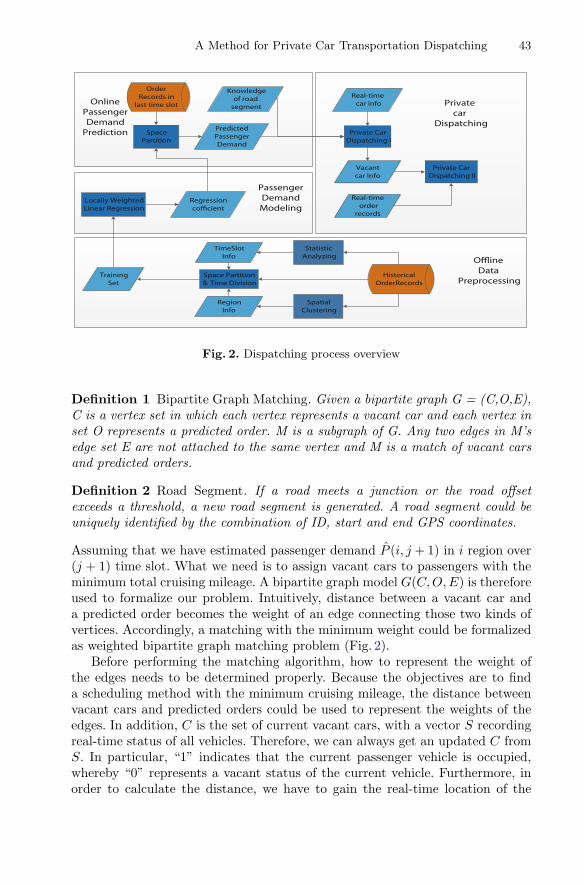
Fig. 2. Dispatching process overview

Definition 1 Bipartite Graph Matching. Given a bipartite graph G = (C,O,E),C is a vertex set in which each vertex represents a vacant car and each vertex inset O represents a predicted order. M is a subgraph of G. Any two edges in M’sedge set E are not attached to the same vertex and M is a match of vacant carsand predicted orders.

Definition 2 Road Segment. If a road meets a junction or the road offsetexceeds a threshold, a new road segment is generated. A road segment could beuniquely identified by the combination of ID, start and end GPS coordinates.

Assuming that we have estimated passenger demand P (i, j + 1) in i region over(j + 1) time slot. What we need is to assign vacant cars to passengers with theminimum total cruising mileage. A bipartite graph model G(C,O,E) is thereforeused to formalize our problem. Intuitively, distance between a vacant car anda predicted order becomes the weight of an edge connecting those two kinds ofvertices. Accordingly, a matching with the minimum weight could be formalizedas weighted bipartite graph matching problem (Fig. 2).

Before performing the matching algorithm, how to represent the weight ofthe edges needs to be determined properly. Because the objectives are to finda scheduling method with the minimum cruising mileage, the distance betweenvacant cars and predicted orders could be used to represent the weights of theedges. In addition, C is the set of current vacant cars, with a vector S recordingreal-time status of all vehicles. Therefore, we can always get an updated C fromS. In particular, “1” indicates that the current passenger vehicle is occupied,whereby “0” represents a vacant status of the current vehicle. Furthermore, inorder to calculate the distance, we have to gain the real-time location of the

44 W. Jiang et al.

vehicle. To deal with this, GPS coordinates are adopted to display the car’sposition. L represents real-time location information of all vehicles. In this way,we can get current status of the car k from Sk and current position from Lk.

With respect to the predicted orders, we use vertex set O to cover orderinformation such as the location to get on the car, expected on-board time,destination etc. In order to simplify the problem, we assume that all orders’expected on-board time is the current time. However, as the exact position ofthe predicted order is unknown, we have to figure out effectively how to estimatea predicted order’s position. As mentioned in Sect. 2, the predicted order countis based on pre-divided region, but region itself is a coarse-grained geographydefinition. Region should be divided in a much more fine-grained manner. Tocope with these issues, we firstly match the historical on-board positions to roadsegment in a region based on historical order analysis. Thereafter, the numberof passengers who boarding on private car in a road segment can be computedand further used to decide which road segment a predicted order belongs to.If the probability of an order appears in a road segment which is greater thana certain threshold value, the order could be definitely identified on the roadsegment. Eventually, the position of the predicted order can be determined bythis road segment.

Moreover, we will discuss how to set the weight of edge. In bipartite graphG (C, O, E), E is the set of edges. Intuitively, the distance between the car andthe order is used to represent the weight of edge between them. Despite otherfactors including the weather, real-time traffic etc., we use Baidu Web APIs toget the shortest distance between two GPS coordinates in our experiment forthe clearness and simplicity of the model.

Given above definitions and descriptions, the scheduling problem could beformalize as a weighted bipartite graph matching problem. Kuhn-Munkras algo-rithm is used to find the optimal matching with minimum cost. Due to the specialnature of KM algorithm, set C and O should have equal vertexes. In fact, wecan add some vertexes to the minimum set on the occasion of two unequal set.Additionally, the weights of edges associated to those added vertexes are set tobe zero. The detailed descriptions of the scheduling process could be found inAlgorithm 2.

After the matching decision, vacant cars will be assigned to the road segmentswhere predicted order exists.

In the real scenario, a real order might be placed while vacant cars are for-warding to a matched road segment. The real order contains information includ-ing the passenger’s position, destination, etc. Meanwhile, vacant cars’ informa-tion can be extracted from vector S and L. In case of the emerging real orders,the closest car will be scheduled and appointed to satisfy the real order demand.Particularly, the status and location of the vehicle need to be updated in real-time manner. Once a vehicle is assigned to a real order, the corresponding statusrelated to real order will be occupied and updated. The status “1” will turn into“0” when the passenger gets off. Finally, the scheduling process proceeds untilall private cars are out of service (finish working).

A Method for Private Car Transportation Dispatching 45

Algorithm 2. schedulePrivateCar()1: initialize each vertex in set C in j+1 time slot;2: predictPassengerDemandInDifferentRegions ();3: initialize each vertex in set O in j+1 time slot;4: find a minimum cruising mileage matching;5: while a real order occurs do6: select vacant cars near the real order’s position;7: if a vacant car accepts the order then8: update car’s status;9: update order’s status;

10: update L and S;11: end if12: end while

4 Experimental Evaluation

In this section, we set up several experiments to evaluate the effectiveness of theproposed passenger demand model and dispatching algorithm.

4.1 Dataset and Experiment Environment

We use a real dataset from a private car hiring company (for commercial rea-sons we cannot identify the name), which contains 2720 vehicles and 356706order records for a whole month in Beijing. The test machine is equipped withDebian 6.0 operation system, 8 GB Memory and Intel i5-4570 with a frequencyof 3.20 GHZ is set up.

4.2 Data Processing

Because the real dataset can not be directly used, the data processing startswith data cleaning and pre-operations. Specifically, we filter the order with atime duration less than 10 min and larger than 60 min, resulting in the remaining324512 records. Subsequently, spatial clustering is utilized to split Beijing urbanarea into multiple regions. To simplify our experiment, DBSCAN algorithm isused to divide urban areas in Beijing four-rings into 136 areas. Two parameters(Epsilon and MinPoints) are set to be 0.15 and 100 respectively according tothe engineering experiences. Actually, the Epsilon indicates the density of aregion, while MinPoints shows how many points a region need to possess atleast. Besides, a day is partitioned into several time slots based on the orderdistribution in one day (Fig. 3).

Figure 4(b) illustrates a good example of regions partition near the BeijingRailway Station and the average count of orders in each time period. We select atime period in which the order count is larger than the average count, leading toa more convenient and reliable prediction. The time duration between 7:00 AMto 10:00 PM is selected as the experimental time interval.

46 W. Jiang et al.

(a) Several regions near Beijing RailwayStation

(b) Average order count in one day

Fig. 3. Regions and time slots

(a) Prediction accuracy (b) Prediction accuracy in regions

Fig. 4. Passenger demand model evaluation

4.3 Model Evaluation

We firstly introduce Non-homogeneous Poisson Process (NHPP) Model. Poissonprocess is a stochastic process that is often used to study the occurrence ofevents. It assumes that the arriving rate of events λ is constantly stable, andhas the Poisson distribution of counting and exponential distribution of inter-event time. In fact, NHPP [6] is a specific Poisson process with a time-dependentarriving rate function λ(t). The model is more flexible and appropriate to depictthe human-related activities because these activities often vary over time buthave strong periodicity. We use ΔT to indicate time increment and N(ΔT ) torepresent order increment in ΔT . Specifically, N(ΔT + j) − N(j) follows thePoisson distribution with a parameter λΔT .

P{N(λT + j) − N(j) = k} =e−λΔT (λΔT )k

k!(8)

Here we set ΔT to one hour and λ can be obtained by maximum likelihoodestimation:

λ =N

ΔT(9)

A Method for Private Car Transportation Dispatching 47

where N can be denoted by average orders in one hour. Therefore, we coulduse the average order count to predict passenger demand. We use the followingequation to calculate the prediction accuracy:

Accuracy =Pi,j+1 − |Pi,j+1 − Pi,j+1|

Pi,j+1(10)

It is observable from Fig. 4(a) that the prediction accuracy of our model out-performs NHPP, and the accuracy in different time periods varies in an accept-able range. Meanwhile, a peak accuracy could be achieved at 18:00. This is dueto an obvious passenger demand trend around 18:00. Figure 4(b) also revealsthe prediction accuracy of different regions. Apparently, the accuracy for Region1 and 2 is steady all the time with little fluctuation. However, the inferenceaccuracy in Region 3 and 4 suffers from some degrees of variations, even withsome outlier results.This is because the number of orders in these Regions are soscarce that the proposed model could not capture a reasonable value. To solvethis problem, we not only enlarge the size of required dataset, but increase theregion’s coverage area as well.

4.4 Dispatching Algorithm Evaluation

In order to replay the real behaviors of the moving vehicles and the user demands,we emulate their moving traces obtained from the historical data and applythem into our algorithms. As shown in Table 2, we choose the real orders andcar traces from 08:00 to 13:00 on May 6th, 2015. At 8:00, there are 324 vacantcars and 296 predicted orders in this evaluation. The result illustrates that theproposed model could finish matching of vacant cars with predicted orders in52 s. In addition, we leverage Baidu Web API to obtain the distance between avacant car and a predicted order with average speed recorded. Once a real orderemerges, the nearest vacant car could be selected to pick up the passenger. Onaverage, 22.5 % cruising miles could be reduced in this simulated experiment.

Table 2. Dispatching results

Time Vacant car count Predicted order count Reduced cruising miles

08:00 325 296 21.5 %

09:00 332 369 23.1 %

10:00 275 285 19.2 %

11:00 247 212 24.9 %

12:00 203 245 27.2 %

13:00 243 210 26.3 %

48 W. Jiang et al.

5 Conclusions and Future Work

At present, taxis in urban areas could not fully satisfy the booming citizens’demand for convenient transportation means. Fortunately, private car hiring isemerging as an alternative and offering a variety of ways for short trips. It isobserved that serving vehicles have to spend a large portion of their servicetime on cruising around streets, resulting in large amountof monetary waste. Tosolve this problem, this paper presents a private car dispatching method basedon a passenger demand model.We use Locally Weighted Linear Regression todepict passenger demands in detail, and formalize private car dispatching as aweighted bipartite graph matching problem. The experimental results demon-strate our model outperforms the non-homogeneous poisson process model witha more stable prediction accuracy. We also exploit a real dataset for simulatingthe private car dispatching process. By using our proposed approach, 22.5 %cruising mileage can be saved. In the future, we will further enlarge our datasetto optimize the proposed model and to take into account other factors affect-ing passenger demands, such as weather, holidays etc. We are also planning toparallelize the dispatching algorithm to reduce further the total execution time.

Acknowledgments. This work is supported in part by China 973 Program (2014CB340300), National Natural Science Foundation of China (91118008, 61170294), China863 program (2015AA01A202), HGJ Program (2013ZX01039002-001), FundamentalResearch Funds for the Central Universities and Beijing Higher Education Young EliteTeacher Project (YETP1092).

References

1. Uber. https://www.uber.com2. Powell, J.W., Huang, Y., Bastani, F., Ji, M.: Towards reducing taxicab cruis-

ing time using spatio-temporal profitability maps. In: Pfoser, D., Tao, Y.,Mouratidis, K., Nascimento, M.A., Mokbel, M., Shekhar, S., Huang, Y. (eds.)SSTD 2011. LNCS, vol. 6849, pp. 242–260. Springer, Heidelberg (2011)

3. Qu, M., Zhu, H., Liu, J., Liu, G., Xiong, H.: A cost-effective recommender systemfor taxi drivers. In: Proceedings of the 20th ACM SIGKDD International Confer-ence on Knowledge Discovery and Data Mining. ACM (2014)

4. Yuan, J., et al.: Where to find my next passenger. In: Proceedings of the 13thInternational Conference on Ubiquitous Computing, pp. 109–118. ACM (2011)

5. Zhang, D., He, T., Lin, S., Munir, S., Stankovic, J.A.: Dmodel: online taxicabdemand model from big sensor data in a roving sensor network. In: 2014 IEEEInternational Congress on Big Data (BigData Congress), pp. 152–159. IEEE (2014)

6. Zheng, X., Liang, X., Xu, K.: Where to wait for a taxi?. In: Proceedings of theACM SIGKDD International Workshop on Urban Computing. ACM (2012)

7. Yuan, N.J., Zheng, Y., Zhang, L., Xie, X.: T-finder: a recommender system forfinding passengers and vacant taxis. IEEE Trans. Knowl. Data Eng. 25(10), 2390–2403 (2013)

8. Ester, M., et al.: A density-based algorithm for discovering clusters in large spatialdatabases with noise. In: Proceedings of International Conference on KnowledgeDiscovery & Data Mining, pp. 226–231 (1996)

9. Chang, H.W., Tai, Y.C., Hsu, Y.J.: Context-aware taxi demand hotspots predic-tion. Int. J. Bus. Intell. Data Min. 5(1), 3–18 (2010)