a method for evaluating the application of variable ...€¦ · figure 2.6 - abb’s acs 1000...
TRANSCRIPT

A METHOD FOR EVALUATING THE APPLICATION OF VARIABLE FREQUENCY DRIVES WITH COAL
MINE VENTILATION FANS
Tyson M. Murphy
Thesis submitted to the faculty of the Virginia Polytechnic Institute and State University in partial fulfillment of the requirements for the degree of
Master of Science In
Mining and Minerals Engineering
Dr. Thomas Novak, Chairman Dr. Antonio Nieto, Committee Member
Dr. Jaime De La ReeLopez, Committee Member
14 April 2006 Blacksburg, VA
Keywords: Mine Ventilation, VFD, Variable Speed, Mine Fan

A METHOD FOR EVALUATING THE APPLICATION OF VARIABLE FREQUENCY DRIVES WITH COAL
MINE VENTILATION FANS
Tyson M. Murphy
ABSTRACT
The adjustable-pitch setting on an axial-flow fan is the most common method of controlling airflow for primary coal mine ventilation. With this method, the fan operates at a constant speed dictated by its motor design. The angles of the blades are adjusted to change the amount of airflow and pressure to meet ventilation requirements. Typically, the fan does not operate at its optimum efficiency, which only occurs in a narrow band of air pressures and quantities. The use of variable frequency drives (VFDs), which control fan speed, provides a solution to this problem. VFDs are already used in various similar applications such as pumping and building ventilation. New technology now enables efficient VFD operation in medium voltage (2,300 – 6,900 V) fan applications. The primary benefit of a variable frequency drive is that it allows motors to operate at reduced speeds, and thus at a lower power, without a loss of torque. VFDs also allow for efficient operation over the entire life of the fan. The technical considerations of using a VFD are presented in this work, along with a method for choosing and modeling a variable speed fan to achieve maximum energy savings. As a part of this research, a spreadsheet program was developed that will calculate the optimum fan operating speed based on given fan data and specified operating conditions. A representative room and pillar coal mine is modeled to illustrate the selection and modeling process and as an example of the economic implications of using a VFD. The use of VFDs is shown to potentially yield large energy savings by increasing the fan efficiency over the life of the mine. Although there are definite power savings while using variable speed fans, the magnitude of these savings is specific to an individual mine and the operating conditions encountered. The determination of whether the use of VFDs is economically feasible requires analysis for the specific mine and its operating conditions. This work provides the background and a method for such an evaluation.

ACKNOWLEDGEMENTS I would like to thank the Department of Mining and Minerals Engineering for the opportunity and financial support for this research. I would like to especially thank Dr. Thomas Novak for his guidance and encouragement. My thanks also go to my committee members Dr. Antonio Nieto and Dr. Jaime De Le Ree for their support, and to Spendrup Fan Company and Reliance Electric for their assistance and information. Finally, I would like to thank my family and especially my fiancée, Crystal, for their patience, love, and support.

TABLE OF CONTENTS Abstract ............................................................................................................................... ii Acknowledgements............................................................................................................ iii Table of Contents............................................................................................................... iv List Of Figures ................................................................................................................... vi List Of Tables .................................................................................................................. viii Chapter 1: Introduction ....................................................................................................... 1
1.1 Problem Statement .................................................................................................... 1 1.2 Proposed Solution ..................................................................................................... 2 1.3 Scope of Research..................................................................................................... 2
Chapter 2: Literature Review.............................................................................................. 3 2.1 AC Motors and Drives .............................................................................................. 3
2.1.1 Induction Motor Principles ................................................................................ 3 2.1.2 Variable Frequency Drive Principles................................................................. 7 2.1.3 Applications of VFDs ...................................................................................... 11
2.2 Mine Ventilation ..................................................................................................... 13 2.2.1 Introduction...................................................................................................... 13 2.2.2 Components ..................................................................................................... 13 2.2.3 Fans .................................................................................................................. 14 2.2.4 Ventilation Analysis......................................................................................... 16 2.2.5 VnetPC Modeling ............................................................................................ 18
Chapter 3: Mine and Ventilation Modeling ...................................................................... 21 3.1 Mine Model Development ...................................................................................... 21 3.2 Ventilation Model Development............................................................................. 24 3.3 Determining the Optimum Operating Point............................................................ 27
Chapter 4: Reduced Speed Fans ....................................................................................... 30 4.1 Selecting an Appropriate Fan.................................................................................. 30 4.2 VFD and Fan Combinations Modeled .................................................................... 32 4.3 Methodology for Modeling Reduced Speed Fans .................................................. 33
4.3.1 Fixed Pitch Fans............................................................................................... 33 4.3.2 Calculating Power and Efficiency ................................................................... 36 4.3.3 Adjustable Pitch Variable Speed Fans............................................................. 41
4.4 Summary of Modeling Results ............................................................................... 43 4.5 Effects of Reduced Speeds on Motors .................................................................... 48 4.6 Summary and Discussion of VFD Effects on Fan Operation ................................. 55
Chapter 5: Economic Analysis.......................................................................................... 60 5.1 Model Comparison Among Options....................................................................... 60 5.2 Additional Considerations ...................................................................................... 63
Chapter 6: Summary and Conclusions.............................................................................. 65 6.1 Future Research ...................................................................................................... 66
References......................................................................................................................... 67 Appendix A: Manufacturer’s Fan Curves......................................................................... 70 Appendix B: Ventilation Schematics................................................................................ 73 Appendix C: Excel program for solving reduced speeds.................................................. 96
iv

Appendix D: Motor Model ............................................................................................. 101 Appendix E: ABB Drive Specifications ......................................................................... 107
v

LIST OF FIGURES Figure 2.1 – Simple Squirrel Cage Induction Rotor (Luttrell 2005)................................... 3 Figure 2.2 – Speed-Torque Profiles .................................................................................... 5 Figure 2.3 – Voltage and Frequency Ratios for Medium Voltages (2300V, 3300V, 4160V, and 6900V)............................................................................................................. 6 Figure 2.4 – VFD Components........................................................................................... 7 Figure 2.5 – PWM waveform ............................................................................................. 9 Figure 2.6 - ABB’s ACS 1000 Variable Frequency Drive topology (ABB) .................... 10 Figure 2.7 – Photograph of ABB’s ACS 1000 Drive (ABB) ........................................... 11 Figure 2.8 – System characteristic curve if R = 0.354x10⁻¹⁰ in·min2/ft6........................... 17 Figure 2.9 – Determining the Fan Operating Point and Power......................................... 18 Figure 2.10 – Mine ventilation plan (Novak 2003) .......................................................... 19 Figure 2.11 – Ventilation network corresponding to the mine plan in Figure 2.10.......... 19 Figure 3.1 – Pillar layout and dimensions ........................................................................ 22 Figure 3.2 – Mine plan general layout .............................................................................. 23 Figure 3.3 – General mine ventilation layout (Novak 2003) ............................................ 25 Figure 3.4 – Ventilation schematic for year 2................................................................... 26 Figure 3.5 – Determining the optimum operating point in VnetPC ................................. 28 Figure 4.1 – Spendrup 274-165-880 fan with yearly operating points ............................. 31 Figure 4.2 – Spendrup 305-183-880 fan with yearly operating points ............................. 32 Figure 4.3 – Iterative process for finding appropriate fan speed ...................................... 35 Figure 4.4 – Reading power from the reduced speed power curves................................. 37 Figure 4.5 – Original Fan Curve with efficiency intersections labeled ............................ 38 Figure 4.6 – Constant Efficiency Zones ........................................................................... 39 Figure 4.7 – Operating Points and Fan Efficiency............................................................ 40 Figure 4.8 – Constant efficiency zones for variable speed and adjustable pitch fans ...... 42 Figure 4.9 – Operating points at pitch settings ................................................................. 44 Figure 4.10 – Constant efficiency zones for Spendrup 305-183-880 fan ......................... 47 Figure 4.11 – Induction motor equivalent circuit ............................................................. 48 Figure 4.12 – Torque of motor operation at 900 rpm ....................................................... 49 Figure 4.13 – Motor efficiency as a function of speed and load factor ............................ 52 Figure 4.14 – Torque produced as a function of speed and load factor............................ 53 Figure 5.1 – Cumulative cash flow – savings over option 1............................................. 62 Figure B.1 – Ventilation Schematic Legend..................................................................... 74 Figure B.2 – Year 2 Ventilation Plan................................................................................ 75 Figure B.3 – Year 3 Ventilation Plan................................................................................ 76 Figure B.4 – Year 4 Ventilation Plan................................................................................ 77 Figure B.5 – Year 5 Ventilation Plan................................................................................ 78 Figure B.6 – Year 6 Ventilation Plan................................................................................ 79 Figure B.7 – Year 7 Ventilation Plan................................................................................ 80 Figure B.8 – Year 8 Ventilation Plan................................................................................ 81 Figure B.9 – Year 9 Ventilation Plan................................................................................ 82 Figure B.10 – Year 10 Ventilation Plan............................................................................ 83 Figure B.11 – Year 11 Ventilation Plan............................................................................ 84
vi

Figure B.12 – Year 12 Ventilation Plan............................................................................ 85 Figure B.13 – Year 13 Ventilation Plan............................................................................ 86 Figure B.14 – Year 14 Ventilation Plan............................................................................ 87 Figure B.15 – Year 15 Ventilation Plan............................................................................ 88 Figure B.16 – Year 16 Ventilation Plan............................................................................ 89 Figure C.1 – Excel Start Page ........................................................................................... 97 Figure C.2 – Program’s primary screen............................................................................ 97 Figure C.3 – Fan curve input ............................................................................................ 98 Figure C.4 – Operating point input ................................................................................... 99 Figure D.1 – Motor performance data, page 1................................................................ 102 Figure D.2 – Motor performance data, page 2................................................................ 103 Figure D.3 – Matlab command window input and output text ....................................... 106 Figure D.4 – Output plot of torque versus time .............................................................. 106
vii

LIST OF TABLES Table 3.1 – Friction factors for coal mine airways (from Prosser and Wallace) .............. 25 Table 3.2 – Optimum operating points for each yearly model ......................................... 29 Table 4.1 – Yearly Speed Requirements........................................................................... 36 Table 4.2 – Reduced Speed Fan Results........................................................................... 40 Table 4.3 – Results from adjustable pitch, reduced speed fan.......................................... 43 Table 4.4 – Operating parameters for Spendrup 274-165-880 fan ................................... 44 Table 4.5 – Results for option 2, adjustable pitch Spendrup 305-183-880 fan ................ 45 Table 4.6 – Results for option 4, fixed pitch Spendrup 305-183-880 fan with VFD ....... 46 Table 4.7 – Results for option 6, adjustable pitch Spendrup 305-183-880 fan with VFD 46 Table 4.8 – Motor performance at reduced speeds over varying loads ............................ 51 Table 4.9 – Fan and motor efficiency comparison ........................................................... 54 Table 4.10 – Summary of scenarios modeled................................................................... 55 Table 4.11 – Total input power requirements, HP............................................................ 56 Table 4.12 – Power difference for each option vs. option one ......................................... 57 Table 5.1 – Capital Costs .................................................................................................. 61 Table 5.2 – Yearly operating costs, $ ............................................................................... 61 Table 5.3 – Net present cost for each option, $ ................................................................ 62 Table 5.4 – Rate of return for each option ........................................................................ 63 Table 5.5 – ROR for lower cost fixed pitch fans .............................................................. 63 Table B.1 – Year 16 branch properties ............................................................................. 90 Table C.1 – Spreadsheet output: Summary of results..................................................... 100
viii

CHAPTER 1: INTRODUCTION
1.1 Problem Statement Primary mine ventilation fans provide necessary airflow and pressure to properly circulate air in the working areas of the mine. During mining, as the size of the mine and mine resistance changes, ventilation requirements will vary as changing airflows are required to maintain a safe mining environment. Usually, the requirements are calculated for different points over the projected mine life, and a fan is chosen that is capable of operating at all of these points over the 15-20 year life of the fan. Missing in this process is a method for dealing with the decrease in fan efficiency at operating requirements that are lower than what the fan is optimally designed for.
The most common primary mine fan is the axial flow type. This type of fan traditionally operates at a fixed speed based on motor design and power supplied to the fan. The power and speed are generally constant for a given fan design. Currently, the most common method of varying the airflow and head of an axial flow fan, in response to the changing conditions of the mine, is to change the pitch of the fan blades (Hartman, et al., 1997). Fan curves are created based on multiple pitch angles for each fan, and a fan is selected that allows for the highest efficiency at changing pitches for the life of the fan.
This method of fan operation results in inefficiencies during the life of the mine. Most often, a mine will operate a fan at a higher airflow than necessary during early mining, simply because it is more efficient than operating the fan at a lower airflow. Nearing the end of mining operations, the fan may be operated near 100% of its capabilities to meet the requirements. In all but a narrow range of airflows and pressures, the fan does not operate at its optimum efficiency.
In addition to the inefficiencies associated with providing adequate airflow, changing the airflow can be an inconvenience to mine operators. Older fans need to be shut down to perform pitch adjustments, while more modern fans can be changed during operation. Regulators are also used to restrict airflow by diverting intake air into exhaust airways before it reaches the faces. Invariably, this results in unused fresh air that is exhausted from the mine.
1

1.2 Proposed Solution Variable frequency drives (VFDs) are one solution to the inefficiencies of current fan operation. VFDs are already used in various similar applications such as pumping and building ventilation. In mining, VFDs have been used in belt haulage systems, continuous miners, and trams. The benefit of a variable frequency drive is that it can allow motors to run at various speeds, without a loss of torque.
The speed of a motor is based on the frequency of the power supplied and the design of the motor. To change the speed, either a physical change in the motor construction or a change in electrical frequency is required. The torque of a motor is determined by both its voltage and frequency, and a motor is rated based on a fixed ratio of these two factors. A VFD can supply power with the proper frequency and voltage/frequency ratio to produce different speeds while maintaining a constant torque in the motor.
The ability to change the speed of ventilation fans is advantageous in controlling the airflow and pressure in a mine. There are many advantages to this approach of controlling airflow. If a VFD is used to control fan speed, energy savings can be realized by operating a fan at a point that meets the ventilation requirements while maintaining high fan efficiency throughout the life of the fan. The use of VFDs also provides flexibility in mine operations by potentially allowing the fan to be adjusted as needed or “on the fly” during mining.
1.3 Scope of Research This research shows the possible benefits of using variable frequency drives in mine fan applications. Technical requirements of ventilation, VFDs, motors, and fans are reviewed to determine the feasibility of installing and using VFDs for mine fan applications. A simple coal mine was designed and modeled to perform a ventilation analysis that incorporates variable speed fans. It is then used to develop and illustrate a method for determining the appropriate reduced speed fan settings to achieve optimum operating conditions. Also of importance are the economic benefits of using a VFD to control fan speed. Although the economics are specific to a single mining operation and its operating conditions, the example mine is used to illustrate some of the trends and issues that are likely to be present.
2

CHAPTER 2: LITERATURE REVIEW
2.1 AC Motors and Drives
2.1.1 Induction Motor Principles AC squirrel-cage induction motors are the most commonly used motors in industry today because of their simple construction, durability, and low cost. As with all induction motors, the basic components of a squirrel-cage induction motor are the stator (stationary winding) and rotor (rotating winding). Instead of an actual winding, a squirrel-cage rotor is simply constructed of longitudinal copper bars connected at their ends by copper shorting rings, as shown in Figure 2.1, hence the name “squirrel-cage.” The entire copper cage is imbedded in a cylindrical magnetic core.
Figure 2.1 – Simple Squirrel Cage Induction Rotor (Luttrell 2005)
When balanced three phase voltages are applied to the windings of the stator, the resulting currents in the windings produce a magnetic field. The speed of this rotating field is referred to as the synchronous speed, nsync (rpm), and is a function of the electrical frequency of the applied voltage, fe (Hz), and the number of poles in the stator, p, as given by the following equation:
p
fn esync
120= (1)
Lines of flux, produced by the rotating magnetic field, cut the copper bars of the rotor, thus inducing current in the rotor bars. The interaction between the stator’s magnetic field and the rotor’s currents results in rotational torque. The rotor then accelerates, with its terminal speed approaching that of the magnetic field. However, the rotor speed can never reach the synchronous speed. If this occurred, the rotor would be traveling at the same speed as the magnetic field and the flux from the magnetic field would not cut the rotor bars. Therefore, no currents would be induced in the rotor, and no rotational torque
3

would be developed. Because of these effects, the mechanical (rotor) speed of the motor must always be less than the synchronous speed of the magnetic field to maintain rotational torque. The speed differential between the synchronous speed, nsync, and the mechanical speed, nm, is defined as a percentage of the synchronous speed, and is referred to as slip, s, given by the following equation:
%100×−
=sysc
msync
nnn
s (2)
As an example, consider an eight-pole motor operating with a rated slip of 2%. Assuming a power line frequency of 60 Hz, the synchronous speed of the motor is
rpmP
fn esync 900
860120120
=×
==
The mechanical speed of this motor is
( ) ( ) rpmsnn syncm 88202.019001 =−=−=
An induction motor operates at relatively constant speed. A typical speed-torque characteristic for an induction motor, along with the load torque for a mine ventilation fan is shown in Figure 2.2(a). As long as the motor torque exceeds the load torque of the fan, the fan will accelerate until the two curves intersect. This point of intersection becomes the operating point of the motor. Induction motors operate at a relatively constant speed with slight variations depending on the load torque, which is a desirable characteristic for a ventilation fan. A significant increase in torque will result in increased slip, and thus a small change in speed (Figure 2.2(b)). If for some reason the load increases, the motor only slows slightly. Since the synchronous speed of the magnetic field remains constant, more lines of flux cut the rotor bars and increase the motor current to accommodate the required increase in torque. An increase in slip thus causes increased current as well as increased torque. It is because of this relationship that high startup currents are present when starting a large motor, from zero rpm to rated speed, and are sometimes as high as 6 to 10 times the operating current (Beaty and Fink 1987).
4

Fan Load Profile
Motor ProfileTo
rque
Speed nm nsync
Operating Torque
Motor Profile
Torq
ue
Speed Δn
ΔT
(a) (b)
Figure 2.2 – Speed-Torque Profiles In order to change the speed of an induction motor, it is necessary to either change the electrical frequency or the number of poles in the motor (Equation 1). Motors require special types of windings with a set of external relays for changing poles. Also, only discrete changes in speed can be achieved with this method. For example, a motor with a synchronous speed of 1200 rpm can be slowed to 900 rpm if the number of poles is increased from six to eight, but speeds between these values can not be achieved. As a result, the technique of changing the number of poles (and thus how the motor is wound) is now obsolete (Chapman 2002), and changing the electrical frequency is the preferred method for varying speed. An important consideration when varying the speed of a motor is to maintain the same torque characteristics of the motor. Torque is proportional to the magnetic flux density in the motor air gap, which is proportional to the ratio of voltage and frequency, and is determined by the motor design. To maintain a constant flux, and thus constant torque characteristics at varying speed, voltage must also be varied to maintain a constant ratio of voltage and frequency. If the voltage is not de-rated as frequency drops, the steel in the core of the motor will saturate, and the magnetization current in the motor will increase and become excessive (Chapman 2002). Equation 3 describes this relationship where V is in Volts, and f is in Hz. Figure 2.3 shows the voltage and frequency ratios for different motor voltage ratings.
cf
V= (3)
5

0
1000
2000
3000
4000
5000
6000
7000
8000
0 10 20 30 40 50 60
Frequency, f (Hz)
Volta
ge, V
(Vol
ts)
c= 115.0c= 69.3c= 55.0c= 38.3
Figure 2.3 – Voltage and Frequency Ratios for Medium Voltages (2300V, 3300V, 4160V, and
6900V)
Losses in the motor consist of stator copper losses, core losses, rotor copper losses, friction losses, and stray losses. The core, friction, and stray losses are usually combined and indicated as rotational losses and are constant with changing speed (Chapman 2002). These losses define the motor efficiency. Efficiency can also be more practically determined by the ratio of power input to power output of the motor, Equation 4.
in
out
PP
=η (4)
6

2.1.2 Variable Frequency Drive Principles Variable frequency drives (VFDs), also referred to as variable speed drives and adjustable speed drives, input line power and output a reduced voltage and frequency supply to the motor. VFDs consist of three major components, as shown in Figure 2.4 – a rectifier/converter to convert AC to DC voltage, an intermediate DC link, and an inverter that outputs a simulated sinusoidal AC voltage from the controlled DC voltage. VFDs use a non-alternating DC voltage internally because it is easier to generate an output waveform (Turkel 1995). Additional input transformers and output filters can be included depending on the drive configuration and design. There are a variety of different ways that these functions are accomplished, but the same basic configuration is used.
M
DC Link Inverter Rectifier
Figure 2.4 – VFD Components The technology used in VFDs has changed greatly over the past 30-40 years, and is now at a point where the advantages outweigh the disadvantages for use in medium voltage applications. High cost and reliability problems, as well as issues of input and output power quality that have prevented the widespread use of medium voltage drives have been resolved (Giesecke and Osman 1999). Giesecke and Osman (1999) also provide what they refer to as the systematic evolution of VFDs and the changing technology that has made VFDs feasible. Advances in the areas of semiconductor switching devices have, in particular, made the use of these drives possible in medium voltage applications. Manufacturers have also embraced this technology, evolving from the approach in the early 1990’s that the drive had to be perfectly matched to the motor by the same manufacturer (Huffman 1990) to manufacturers that will now make VFDs that are capable of retrofit on any AC motor. A listing of VFD topologies is shown below (Morris and Armitage), with a brief listing of advantages and disadvantages with regard to medium voltage applications. The topology of a VFD is the electrical configuration of the drive, which ultimately determines the overall function of the drive. Motor control platforms, which are a part of the converter
7

section of the drive, determine how energy is delivered to the motor, and control the speed and torque delivered (Morris and Armitage). Emphasis is placed on topologies and motor control of medium voltage systems for fan and pump applications, since that is the focus of this research. Examples of Drive Topologies:
- Voltage Source Inverter (VSI) – Advantages: Can retrofit on existing motors without derating, full torque at low speeds, input power factor near unity, low network harmonics, and high efficiency.
- Current Source Inverter (CSI) – Advantages: Cost effective, four quadrant operation. Disadvantages: Continuous low speed operation not possible, inconsistent power factor over operating range, higher cost, larger drive, and additional losses.
- Load Commutated Inverter (LCI) – Advantages: Single Motor Drive for medium and high power ratings, wide speed and power range, inherent 4-quadrant operation. Disadvantages: Not for use on squirrel cage induction motors.
There are two primary motor control platforms used in VFD applications. The first is Pulse Width Modulation (PWM). This platform uses a pulse width modulator to simulate a sine wave, with the voltage and frequency determining the torque and speed. The output is a series of pulses of varying widths. The width of each pulse controls the magnitude of the voltage and the frequency of the changing polarity of the pulses control the frequency of the power delivered (Yaskawa Electric America). Figure 2.5 shows a PWM line diagram with the corresponding desired waveform. The ongoing development of power devices and increased use has made PWM VSI converters relatively inexpensive (Shakweh 2000).
8

time
Volta
geDesired waveform
PWM waveform
Figure 2.5 – PWM waveform
A few semi-conductor switching technologies that exist in VFD applications are:
- GTO – Gate Turn Off Thyristor - IGBT – Insulated Gate Bipolar Transistor - SGCT – Symmetrical Gate Commutated Thyristor - IGCT – Integrated Gate Commutated Thyristor
GTOs were initially used in VFDs, but were not successful due to their expense and complexity. IGBT technology has been significantly improved for use in medium voltage applications and is a popular choice of technology for VFD manufacturers. According to ABB, who pioneered the IGCT, their technology is ideal for medium voltage drives primarily due to faster switching and lower power dissipation, resulting in its high efficiency and reliability, and reduced size and cost compared to IGBTs (ABB). Regardless of manufacturers’ claims that their technology is superior to the competition, both IGBTs and IGCTs are viable technologies and are both being continually improved. Direct torque control (DTC) is a more recently developed motor control platform, especially for medium voltage drives. DTC controls speed and torque directly, without the use of a modulator. DTC can catch a load already in motion, providing the ability to resume fan operation after an interruption in power without waiting for the fan to come to a stop (Morris and Armitage). DTC accomplishes this by using motor flux and torque as primary control variables that are compared to values from an internal motor model. Adjustments are made to the voltage and frequency accordingly. This process does not
9

require an actual speed measurement to be taken, thus requiring no feedback and eliminating any feedback encoder failure (ABB). The actual operation of DTC is beyond the scope of this research, but Buja and Kazmierkowski present a review of DTC techniques and their operation (Buja and Kazmierkowski 2004). VFDs that are based on the VSI PWM technology inherently have four disadvantages that require additional motor considerations – internal temperature increases, breakdown of the insulation in the windings, bearing currents, and harmonics and electromagnetic interference (deAlmeida et al. 2004). A solution to these problems is to use a sine wave output filter. The filter is located between the drive and the motor, and has the following benefits: no extra motor stress, no insulation stresses or cable resonances, minimal currents to ground or bearings, minimal noise, and can utilize standard motors (Shakweh 2000). This last point is especially important, as it allows VFDs to be installed on existing motors without modifications or additional costs. Another option is a VFD incorporating IGCT technologies with output filters, which offers nearly sinusoidal output and a rapid response to torque variations, resulting in no motor derating, and no additional winding insulation (Steinke et al. 1999). By utilizing DTC, the starting torque is maximized and fluctuations in load are compensated for with a quick response. These features also allow the drive to be used on nearly any motor, including retrofitting motors in existing applications. An example of the topology of a modern VFD is shown in Figure 2.6 below, and a photograph of the same drive is pictured in Figure 2.7. This drive is ABB’s ACS1000 medium voltage drive.
© 2005 ABB MV Drives
Figure 2.6 - ABB’s ACS 1000 Variable Frequency Drive topology (ABB)
10

© 2005 ABB MV Drives
Figure 2.7 – Photograph of ABB’s ACS 1000 Drive (ABB)
2.1.3 Applications of VFDs Variable frequency drives are common in many different industries today. The benefits of a VFD are widely utilized in various applications. In the mining and mineral processing industry, VFDs are used for operating belt conveyors, mills, and pumping, as well as trams and continuous miners. There are three basic categories of motor load which are classified based on how torque requirements vary with speed (Allen-Bradley).
1) Constant torque load – The torque is constant at all speed ranges, and the horsepower is directly proportional to speed. These applications are essentially friction loads, such as conveyors and extruders, high inertia loads, and positive displacement pumps.
2) Variable torque load – The torque is low at low speeds, and high at high speeds. Usually the torque is a function of speed squared. Applications with this load profile are fans, pumps, and blowers.
3) Constant horsepower load – Speed and torque are inversely proportional: high torque at low speeds and low torque at high speeds. This load is a function of the
11

motor being operated above base speed, and applications include winders and machine tool spindles.
The variable torque applications are ideal for achieving energy savings with the use of a VFD (Huffman 1990). Usually these devices operate with a constant speed motor, and use throttling devices such as dampers or valves to control flow by increasing pressure, which then increases the motor load and motor power. Energy savings are realized by avoiding the use of throttling devices and by instead controlling flow via motor speed. The primary benefit of using VFDs on constant torque applications is to improve the response and accuracy of the process (Huffman 1990).
12

2.2 Mine Ventilation
2.2.1 Introduction The purpose of mine ventilation is to help maintain a safe and healthy environment underground that provides a reasonable comfort level (McPherson 1993). Adequate airflow is necessary to provide fresh air for miners to breathe and to remove harmful gases and dust. In coal mines especially, there are many federal and state regulations that govern exactly how this is to be accomplished. There are maximum dust and gas concentrations that must be maintained in the mine, thereby creating specific airflow requirements in certain areas. Fans located in either the mine or on the surface, provide this necessary airflow and are an essential part of this ventilation system. As the mine is developed and the expanses underground increase, the ventilation system must also be able to adapt over time to the changing conditions. A great deal of engineering goes into developing a mine ventilation system to incorporate all of these factors. Behind meeting all safety and regulatory standards, economics also play a large role in how a ventilation system is created. There has been much research on the principles and methods of mine ventilation. Below is a brief overview of the components of a simple room and pillar mine ventilation system, and how one is developed.
2.2.2 Components Airflow is generated by large mine fans and travels through the mine workings, usually from an intake shaft to an exhaust shaft. In the mine, air direction and quantity are controlled by a variety of devices. Permanent and temporary stoppings are used to block passages, regulators reduce the flow of air by partially blocking an airway and creating a shock loss, and over- or under-casts allow air to cross at intersections without mixing. These devices are used below in a description of a simple room and pillar coal mine. In room and pillar mining, the mains and panels are separated into parallel airways by the placement of stoppings. These stoppings are physical barriers used to prevent mixing of air, and are either temporary or permanent (Hartman et al. 1997). These airways are used for intake, return, or neutral airflow, depending on the number of entries in the section. An example is illustrated with further detail in the Chapter 3. Air flows from the intake shaft into the mains. From the mains the air is split to travel through each panel to the working face. In Figure 2.4, the layout employs a double split method where the intake air flows through the center entries, is split at the face, and is
13

returned via each outer entry. Regulators in the panel returns will limit the amount of air that enters each panel, and will keep air from short circuiting through the first available panel off of the mains. These regulators will optimally be set to allow only the minimum required airflow to reach the face. Neutral airways usually contain the belt conveyor. Airflow can also be controlled at the fan with the use of baffles or dampers, or by changing the pitch of the fan blades. In coal mines, standard practice is to place the primary mine fan at the exhaust of the system on the surface (Vutukuri and Lama 1986). In non-coal mines, if necessary, smaller booster fans can be located in the airways to provide sufficient airflow at certain locations.
2.2.3 Fans Primary mine fans are generally either centrifugal fans or axial flow fans. Most fans today are of the axial flow type (Hartman et al. 1997). The characteristics of a fan are determined experimentally by the fan manufacturer. For a given size fan at its rated speed and a constant air specific weight, these characteristics are commonly represented in the form of ‘fan curves’ or plots of head, power, and efficiency versus quantity. Examples of actual fan curves can be found in Appendix A. Fan curves are generated from performance testing data collected by the manufacturer, and are valid for only the fan and conditions tested. These curves account for leakage and other losses and inefficiencies in the fan, and represent values lower than those found by theoretical calculations. Since the fan curves are generated for a specific size fan at a specific speed, to find the characteristics of a fan operating at a different speed or size requires additional calculations. McPherson (1993) describes the theory and derivations of the dimensional analysis that yields a set of relationships known as fan laws (Equations 4-6). These laws allow a new fan curve to be generated while changing one or more operating conditions. In each of these cases, the fan efficiency remains constant since the air power and brake power vary proportionally (Hartman et al. 1997).
3nDQ ∝ , or 3
1
2
1
2
1
2⎟⎟⎠
⎞⎜⎜⎝
⎛=
DD
nn
QQ (4)
14
wDnH 22∝ , or 1
2
2
1
2
2
1
2
1
2
ww
DD
nn
HH
⎟⎟⎠
⎞⎜⎜⎝
⎛⎟⎟⎠
⎞⎜⎜⎝
⎛= (5)
wDnP 53∝ , or 1
2
5
1
2
3
1
2
1
2
ww
DD
nn
PP
⎟⎟⎠
⎞⎜⎜⎝
⎛⎟⎟⎠
⎞⎜⎜⎝
⎛= (6)
where, Q = airflow
H = head/pressure P = motor power D = fan diameter n = fan speed w = air specific weight subscript 1 = values with initial parameters/conditions subscript 2 = values at changed parameters/conditions
Measuring fan performance as a function of power results in an expression of fan efficiency. The mechanical efficiency, η, is expressed as Equation 7, where Pa is the air power, and Pm is the brake power.
%100×=m
a
PPη (7)
Air power can be calculated from the head, H, and quantity, Q. In English units (H in in. WG and Q in cfm), the formula is Equation 8. Brake power is the power that must be supplied to the fan, and is found by multiplying the fan efficiency by the air power. Brake power can also be simply read from the manufacturer’s fan curves or calculated from the fan laws (Equation 6).
hpHQPa 6346= (8)
15

2.2.4 Ventilation Analysis In order to provide the necessary airflow, the fan must generate a high enough pressure to overcome the resistance of the mine airways. This pressure, or head loss, is a function of the airflow and the size, length, and friction factor of each airway section in the mine. Head loss can be related to airflow and these airway parameters by Atkinson’s equation, Equation 9. The total head loss for the mine is found by combining (in parallel or in series) all individual airway losses based on Kirchhoff’s laws. Hartman (1997) and McPherson (1993) describe this process in detail in their books.
( )3
2
2.5 AQLLKOH e
l+
= (9)
Where, Hl = Head loss, in. WG
K = Friction factor, lb·min2/ft4 O = Perimeter, ft L = Length, ft Le = Equivalent length of shock losses, ft Q = Airflow, ft3/min A = Area, ft2 Values for friction factors vary depending on the type of mine, how the airways are supported, and the airway condition. The head loss is directly proportional to the square of the quantity of air (Equation 9). If K, O, L, Le, and A are held constant, they can be combined to form one single constant, R, or the resistance of the airway (Hartman et al. 1997). Equation 9 can then be rewritten as: (10) 2RQHl =
Since the resistance is constant at given operating conditions, this equation can be used to define the characteristics of the mine over a range of pressures and airflows. The resulting graph of such a calculation (Figure 2.8) is known as the system or mine characteristic curve, which describes the head loss at any quantity of airflow.
16

0.0
0.5
1.0
1.5
2.0
2.5
3.0
3.5
0 50 100 150 200 250 300 350
Airflow, kcfm
Hea
d, in
. w.g
.
Figure 2.8 – System characteristic curve if R = 0.354x10⁻¹⁰ in·min2/ft6
By overlaying the system characteristic curve with the fan characteristic curve, a fan operating point can be found (Figure 2.9). This point corresponds to the pressure and quantity of air that the fan will provide based on the resistance of the mine. Power requirements can be found from the fan curves by reading the power at the same airflow of the operating point.
17

0.0
0.5
1.0
1.5
2.0
2.5
3.0
3.5
0 50 100 150 200 250 300 350
Airflow, kcfm
Hea
d, in
. WG
0
10
20
30
40
50
60
70
80
90
100
Bra
ke P
ower
, HP
Operating point
Operating power
System Curve Fan Curve
Power Curve
Figure 2.9 – Determining the Fan Operating Point and Power
2.2.5 VnetPC Modeling VnetPC is a ventilation modeling program developed by Mine Ventilation Services, Inc. This software takes data that describes the mine airways (length, friction factor, geometry) and fan properties (H-Q characteristic) to generate a ventilation model that includes fan operating points, regulator/booster requirements, airway quantities and resistances, and power requirements. The branch data entered into the program is based on a ventilation network representation of the mine that consists of branches (mine airways) and nodes (intersections of airways). Branches are defined by their respective node endpoints. This topology represents a simplified layout of the actual mine. Each branch has properties associated with it, including length, resistance per unit length, parallel airway factor, type of airway, and surface state. Figure 2.10 shows a segment of mains and a panel from a mine plan. Figure 2.11 illustrates the corresponding ventilation network. The ventilation layout combines parallel airways into a single flow path and only includes nodes where airways combine or split. Stoppings are modeled as sets of parallel airway leakage paths, with a single high resistance corresponding to the number of stoppings modeled per path (Bruce and Koenning 1987). The ventilation network is not to scale because the lengths of branches between nodes are a property of each branch.
18

Figure 2.10 – Mine ventilation plan (Novak 2003)
Figure 2.11 – Ventilation network corresponding to the mine plan in Figure 2.10 The program numerically calculates the head losses and quantities of each airway, and determines an overall mine resistance. The process behind this is based on the Hardy-Cross iterative method to determine an optimal solution. The procedure is as follows, summarized from the VnetPC2003 Help File (Mine Ventilation Services 2003):
19

1) The code creates a number of closed loop meshes based on the number of branches and nodes present in the model. 2) For every mesh, an airflow quantity correction factor is calculated using airway resistances and fan pressures. The program estimates an initial airflow and the simulation is initiated. 3) The airflow correction factor is applied to the flows of all the branches in the mesh. This is performed for each mesh in the network. 4) This process is repeated iteratively until Kirchhoff's Second Law holds to a prescribed level of accuracy for every mesh in the network. The resulting network is then balanced.
With user inputted fan curve points, VnetPC also calculates the operating point of the fan. Using VnetPC greatly simplifies complex calculations and allows for changing conditions or different fans to be modeled quickly and easily.
20

CHAPTER 3: MINE AND VENTILATION MODELING
3.1 Mine Model Development To simulate the effects of varying fan speed, a simple room and pillar coal mine was designed to serve as the basis for the ventilation analysis. The actual design is not critical to this research because only comparisons of fan configurations are studied. The design used for this model can be replaced with any mine plan, and the results should have similar trends. The mine design is simple and straightforward so that the changes in ventilation requirements are due to mine development and distance from the fan over time. Since the objective of this study is to simulate the effects of changing the fan speed, special configurations, multiple ventilation shafts, and multiple fans are avoided. The mine design results in ventilation requirements that increase with mine development over time. Although the coal mine modeled is not based on an actual mine, typical data were used for describing the ventilation characteristics. It is assumed that the coal seam is 6 ft thick and extends over a large area, at a depth of approximately 800 ft. An average coal density of 80 lb/ft3 was also assumed. The mine plan developed for this seam is a standard room and pillar layout. Pillar dimensions are 80 ft x 80 ft developed on 100 ft centers, with a 5 entry panel and 8 entry mains, illustrated in Figure 3.1. An 80 ft barrier between panels is maintained. Access to the mine will consist of 18 ft diameter intake and return shafts, as well as a 14 ft x 14 ft dual compartment slope at an angle of 17º.
21

Figure 3.1 – Pillar layout and dimensions
To develop a reasonable timeline for mining this seam while simplifying the ventilation model, a few basic operating parameters had to be determined. For this room and pillar mine, two continuous miners will be used, each with an average production capability of 1,100 tons per shift. At two shifts per day, and 300 operating days per year, production totaled 1.3 M tons per year. Panel length was determined by an increment of the distance a continuous miner could cover in one year, including time for development of the mains ahead of the panels. Excluding the 1000 ft of mains ahead of the panels, each miner can cover approximately 15,600 linear feet of mining in a year. By using a panel length of 7,800 ft, each miner will mine two full panels per year. For simplicity, pillar extraction is not used, and after each panel is mined out, it is then sealed. The average operating life for a primary mine fan is between 15 and 20 years, therefore, the objective was to study the mine over a 15 year life. A portion of the resulting mine plan is shown below in Figure 3.2.
22

Figure 3.2 – Mine plan general layout
23

3.2 Ventilation Model Development Because of the simplicity of the mine layout, only one intake and one return shaft were used in this model. For the ventilation modeling, it was assumed that there would only be one continuous miner operating per panel, resulting in the design of two panels mined simultaneously. From a ventilation standpoint, the worst conditions result from having a miner at the end of each panel at the same time. At this point in time, the air must travel the farthest distance from the shaft to the last open crosscut in each active panel. The conditions at this point were the conditions assumed for the development of the ventilation model. Ventilation requirements in the model include:
• Maintain a minimum airflow of 50,000 cfm at the last open crosscut at each panel. • Maintain a minimum airflow of 3,000 cfm at the tailpiece of each belt. • Maintain an average airflow of 5,000 cfm at the last open crosscut at the end of
the mains when development is not occurring. • Velocity in the intake airways must fall within the recommended range of 600-
1150 fpm (Mutmansky and Greer 1984). Regulators are placed in the returns of each panel to control the airflow at the last open crosscut. Control devices are also placed at the belt tailpieces to limit the airflow. In VnetPC, these locations are modeled as branches with a fixed quantity, where regulators or booster fans are added as necessary to maintain the specified airflow. Values for the friction factor in each airway vary widely based on the conditions at each mine. These values have been researched by a number of people, and a recent study by Prosser and Wallace (1999) provided the values for coal mine airways, listed in Table 3.1 below, used in this research. The authors identify average values and standard deviations from a series of measurements, but to be conservative, the values used in this research represent their average values plus one half of the standard deviation, as is recommended by the authors.
24

Table 3.1 – Friction factors for coal mine airways (from Prosser and Wallace)
AirwayFriction Factor
(lb·min2/ft4 x10-10)Intake 46Return 52Belt 74
A dual split configuration is used in both the mains and the panels (Figure 3.3). Equalizers are located every 2000 ft along the mains to connect the returns along each side of the mains. This practice allows the airflows to balance in each return and offers an alternative path for airflow if a return becomes blocked. The belt is isolated from the intake and returns, and is considered a neutral airway. Since the panels are sealed after they are mined out, only the farthest panels along the mains have an effect on ventilation requirements.
Figure 3.3 – General mine ventilation layout (Novak 2003) To compare and contrast fan and VFD configurations over the life of the mine, a yearly time interval was modeled. Any time increment could have been used, but since each time interval required separate models, a yearly increment was deemed sufficient to allow the effects of using VFDs to be perceptible. A separate ventilation model was created for
25

each year of the 15 year mine life. These models represent the extent of mining at the end of the year at the most demanding conditions, as described above. The sequencing of models starts at year two, allowing for a year for initial development. The schematic for year two is shown below in Figure 3.4 and the schematics for years 3-16 are contained in Appendix B. Intersections of airways are indicated with a dot and node number. For these schematics, any airway intersections that are not numbered do not intersect. As illustrated in the schematics, the only significant difference between the yearly models is the distance of the active panels from the shaft (i.e. the length of the mains). The scheduling allows for the mains to be developed 1000 ft in front of the panels at each year.
Legend Node Numbering: 100’s, 500’s = Intakes 200’s, 400’s, 600’s = Returns 300’s, 700’s = Neutral R = Regulator --- = Stoppings Leakage
Figure 3.4 – Ventilation schematic for year 2
26

3.3 Determining the Optimum Operating Point To provide a standard for comparison, the optimum operating point was required for each model. This ‘optimum’ can be defined as the operating point which results in the lowest head and quantity produced by the fan to adequately supply each face with the required air quantity. There has been much research into determining this optimum point, and devising ways to calculate it. For example, there are methods that favor linear modeling and others that prefer using non-linear models to solve the ventilation network and determine the losses at each regulator and find the fan operating point to balance a network (Jacques 1991; Zhuyun and Yingmin 1991). Most of this research does not consider actual power costs though, and only attempts to optimize the ventilation network and fan conditions with regulator settings. A succinct explanation of how to find the optimum operating point is to “minimize the work performed by all fans in the ventilation network while minimizing energy losses at all regulators,” (Krzystanek and Wasilewski 1995). Although Krzystanek and Wasilewski do not propose a method to determine this, their process leads to the conclusion that reducing the overall amount of regulation results in an increase in the efficiency of the ventilation system, accompanied by a decrease in the required head and quantity of the fan. This increase in efficiency can be directly related to energy savings, as operating a fan at a lower head and quantity results in lower power consumption. For this research, it was not practical to develop a computer program that would account for variable speed fans or even to redesign current computer programs for the same effect, but it was feasible to use VnetPC to solve this problem in a slightly different manner. The program solves the ventilation model based on either a given fixed fan pressure or a fan curve, and sizes the regulators to ensure adequate ventilation. By iteratively varying the fan pressure and calculating the solution, the fixed quantity branches can be monitored, and the optimum operating point determined when a fan pressure yields a minimum sum of regulator resistance in these branches. Three iterations of this process can be seen in Figure 3.5. VnetPC replaces regulators with booster fans in the fixed quantity branches if the overall fan pressure is too low to supply the required airflow, shown in iteration 1. Thus, ideally, the fan pressure can be reduced until the regulators furthest from the intake shafts will behave like a free split, and have zero regulation.
27

Iteration 1
Iteration 2
Iteration 3
Figure 3.5 – Determining the optimum operating point in VnetPC
From the models used in this research, it was impossible to achieve exactly zero regulation in a fixed quantity branch, but it was possible to find the lowest fan pressure to an accuracy of 0.01 in. water gauge that did not turn the regulator into a booster fan. This process was repeated for each yearly model, and the corresponding airflow of the fan was recorded with each pressure. A summary of these optimum operating points is in Table 3.2. To confirm the proper fixed quantity settings (and amount of regulation) at the optimum operating points, the branch results were reviewed to ensure that the ventilation requirements of the belt tailpieces and last open crosscuts met the specifications.
28

Table 3.2 – Optimum operating points for each yearly model
YearQuantity,
kcfmHead, in.
WG2 219 1.703 231 2.024 244 2.375 257 2.726 270 3.097 286 3.568 305 4.149 324 4.7610 347 5.5311 366 6.2312 392 7.1913 417 8.2214 447 9.4915 474 10.7416 509 12.41
Any fan operating point that meets these minimum conditions will adequately supply the mine with ventilation, but any point higher than these this will result in a loss of fan efficiency.
29

CHAPTER 4: REDUCED SPEED FANS Once the ventilation model was created and the optimum operating points were found, the next stage of the research was to determine the speed at which to operate the fan to meet the ventilation requirements while maximizing the fan and motor efficiency. This was accomplished by first choosing an appropriate fan, and then creating reduced speed head-quantity, power, and efficiency curves. The following sections detail each of these steps.
4.1 Selecting an Appropriate Fan The choice of an appropriate fan is based on the manufacturer’s fan curve data. A fan is selected based on an available pitch setting that will satisfy the mine’s most extreme operating condition at an acceptable efficiency. In practice there is no single optimum fan for a given mine, but rather, many fans constructed by different manufacturers will meet the specifications determined by the mine. The definition of ‘optimum’ is also specific to the mining operation, but below are additional points to consider when choosing a fan for use with a VFD. Comments on fixed pitch fans are included, and refer to fans that can be manufactured without any provisions for adjusting the pitch setting of the fan blades. Although at this point in time, the cost of a fixed pitch fan is the same as an adjustable pitch fan (Spendrup 2005), there is the prospect that an increased demand for fixed pitch fans might be incentive for manufacturers to produce them for a lower cost. For fixed pitch fans:
• The maximum efficiency that can be obtained at this fan setting will be the maximum efficiency achievable at any operating point while using a VFD as well. For fans with similar costs, choose the one that provides the highest efficiency.
• In most cases, the best fan will meet the most extreme operating condition while operating near its maximum capabilities at an acceptable efficiency.
• Depending on the lifetime operating conditions, it might be more economical to use a fan that will meet the maximum operating conditions at the center of its efficiency “bubble” (resulting in operation at a point well below its maximum capabilities), rather than one that meets the operating conditions at a lower efficiency. Choosing a fan that is larger than necessary to provide adequate
30

airflow might require higher capital expenses, but maintaining a high efficiency in each year will result in savings that might offset the additional expense.
For adjustable pitch fans:
• A fan that will meet the requirements for a fixed pitch fan can be the best option for adjustable pitch fans.
• The limitations of the maximum achievable efficiency in each year are reduced, providing a greater range of operating conditions that fall within the larger efficiency zones.
• Using the same size fan as with fixed pitch, it is usually possible to increase the fan efficiency for each operating point by adjusting the pitch. Ultimately, economics (capital costs) will determine whether an adjustable pitch or fixed pitch fan should be used.
For the mine modeled in this research, a Spendrup Series 274-165-880 fan was found to provide adequate ventilation capabilities at an acceptable efficiency. This is a 108 in. diameter fan that operates at 880 rpm. The yearly operating points are shown with the manufacturer’s fan curves in Figure 4.1.
0 100 200 300 400 500 600 7000
2
4
6
8
10
12
14
16
0
300
600
900
1200
1500
234
56
78
910
11
12
13
14
15
16
654
32
Fan
Tota
l Pre
ssur
e, in
. w.g
.
Fan Flow Rate, kcfm
1
70%
75%80%85%
1
6
5
43
2 Bra
ke H
orse
pow
er, H
P
Figure 4.1 – Spendrup 274-165-880 fan with yearly operating points
31

An additional Spendrup fan, model 305-183-880, also provides adequate ventilation, but at a lower overall fan utilization. This is evident from Figure 4.2 which shows that the maximum operating conditions only occur at approximately 50% of the fan’s capabilities. As noted in the suggestions for fan selection, above, this larger 120 in. fan meets the maximum ventilation requirements at a higher efficiency than the smaller Spendrup 274-165-880 fan (84% vs. 78%).
0 100 200 300 400 500 600 700 800 900 10000
2
4
6
8
10
12
14
16
18
20
0
500
1000
1500
2000
2500
3000
2345
67
89
1011
12
13
14
15
16
654
3
2
Fan
Tota
l Pre
ssur
e, in
. w.g
.
Fan Flow Rate, kcfm
1
70%
75%
84% 80%
5
6
43
2
Bra
ke H
orse
pow
er, H
P
1
Figure 4.2 – Spendrup 305-183-880 fan with yearly operating points
4.2 VFD and Fan Combinations Modeled To determine whether the size/capacity of the fan has an overall effect on the performance of fans with VFDs, multiple scenarios were modeled for the mine plan described in Chapter 3. For this analysis, six different fan and VFD scenarios were modeled. They will be referred to as options 1 through 6, and are described below. These options attempt to illustrate the performance results of using VFDs and/or adjustable pitch fans on the mine modeled in the previous sections. Even though actual
32

performance results are specific to the mine, trends and patterns can be illustrated by comparing the options relative to each other with this example. Options Modeled:
1. Use the Spendrup 274-165-880 fan as a standard adjustable pitch fan operating in a conventional manner. This option is likely to be similar to the typical choice of fan to meet the requirements of the example mine.
2. Use a larger Spendrup 305-183-880 fan as a standard adjustable pitch fan in a conventional manner. This option would not likely be chosen, as the fan is not fully utilized and costs are unnecessarily higher.
3. Use the Spendrup 274-165-880 as a fixed pitch fan with a VFD. This option was modeled to show performance differences if a fan were manufactured that had one fixed blade pitch setting. Costs could be lower if the fan did not require adjustable pitch settings. It was assumed that the pitch was fixed at setting number 6.
4. Use the Spendrup 305-183-880 as a fixed pitch fan with a VFD. This option is modeled for the same reasons described in option 3. This fan was assumed to be fixed at pitch setting number 4.
5. Use the Spendrup 274-165-880 fan as manufactured as an adjustable pitch fan and operating at reduced speeds with a VFD.
6. Use the Spendrup 305-183-880 fan as manufactured as an adjustable pitch fan and operating at reduced speeds with a VFD.
4.3 Methodology for Modeling Reduced Speed Fans
4.3.1 Fixed Pitch Fans For the analysis and plotting, tables of data points (or equivalent equations) of the fan curves are required. If standard manufacturer’s hard copy or digital (i.e. PDF) graphs are used, scanning and then digitizing the curves is necessary. Resulting data tables should include points along each of the fan curves, power curves, and any intersections of the fan curves and efficiency lines. If the fan has a fixed pitch, then only the curve for that pitch setting is useful. The general process for creating these reduced speed fan curves follows. The Spendrup series 274-165-880 fan was used in the example to describe the process throughout this
33

section. The same process was used for the Spendrup series 305-183-880 fan, with the values of fan performance changed. All of the results are presented collectively after the process is described. From the original fan curves, Figure 4.1, it was determined that pitch setting number 6 is required to meet the maximum operating conditions with a resulting efficiency between 75 and 80%. Using the fan laws for quantity, head, and power (Equations 4 through 6), a new fan curve and power curve can be calculated in a spreadsheet for any new speed from each data point on the original curve and the original design speed. Finding this appropriate speed for each operating point is an iterative process, requiring the equation of the mine resistance, and the equation of the fan curve. The mine resistance at the optimum operating point can be calculated from the mine head and total quantity by Equation 10. Using this resistance, an equation (of the same form) for the mine resistance can be created for head as a function of quantity. For example, if R = 0.354x10⁻¹⁰ in·min2/ft6, the resulting equation for mine head is: 21010354.0 QH ××= −
The process to obtain the approximate equation of the fan curve involves general curve fitting. The data points along the curve are known from the digitized fan curve, and the form is approximately quadratic. The equation relating head, H, to quantity, Q, is: (11) 3
21 2 cQcQcH fit ++=
Where, c1, c2, and c3 are constants
This curve fitting is performed using Microsoft’s Excel Solver add-in. The constants are adjusted automatically by the Solver algorithm until the sum of squares difference between the fit values of head and actual values of head is minimized. Using the previous two equations relating the head and quantity of the mine and the fan, an intersection point can be found by solving both equations simultaneously within the range of the fan’s operating quantity. This point indicates the operating point of the fan for the given mine resistance at the specified speed. The process of curve creation to finding the operating point was repeated iteratively using a binary search method until a speed was found that resulted in a difference between the
34

calculated and specified operating point’s head and quantity of less than 0.5%. Although the resulting speeds were found to an accuracy of 1 rpm, values were reported to the nearest increment of 5 rpm. By this process, a speed was found for each operating point (yearly interval) over the life of the mine, as summarized in Table 4.1. This entire procedure was done using Excel. Macros were set up to use Solver to automate the curve fitting and iterative search process. The resulting spreadsheet was then constructed to be accessed through user forms, allowing all calculations to be performed by a simple click of a command button for each yearly operating point, or for all years sequentially. Details of this spreadsheet and macros are included in Appendix C. A visual representation of the iterative process is shown in Figure 4.3. The dot on the system curve is the optimum operating point, and the intersection of each reduced speed fan curve with the system curve represents the operating point at that speed. It can be seen then that the optimum operating point can be achieved at a fan speed of 350 rpm.
0
0.5
1
1.5
2
2.5
3
3.5
0 50 100 150 200 250 300 350
Fan Flow Rate, kcfm
Fan
Tota
l Pre
ssur
e, in
. w.g
.
400 RPM
375 RPM
350 RPM
325 RPM
System Curve
Figure 4.3 – Iterative process for finding appropriate fan speed
35

Table 4.1 – Yearly Speed Requirements
Year Speed, rpm1 3502 3503 3754 4005 4256 4507 4808 5159 55010 59011 62512 67013 71514 76515 81516 875
It was also important to check the ventilation model’s branch results to verify the spreadsheet calculations are correct and ensure that the minimum airflow requirements are being met at the designated branches. At lower pressures, the fixed quantities of the regulators required only small adjustments to accomplish this. The process involved inputting the new reduced speed fan curve into VnetPC, and executing the model. If the quantities at the faces were inadequate, the regulators were adjusted and the model re-executed. The fan results were recorded, and the process repeated at each yearly interval. The significant results from this modeling were the fan quantity and head, as well as the air power required, and are summarized in Table 4.2 in the next section.
4.3.2 Calculating Power and Efficiency After the required speeds and resulting fan curves were determined, the brake power for each operating point was then found. There are two methods to find this value. First, the yearly operating points were plotted on a graph that included each reduced speed power curve. The value of power was then read from the graph at each yearly quantity. For example, at year 14, the brake power is approximately 875 hp, as read from the graph in Figure 4.4. However, this reading is only as accurate as the scale on the graph. For better accuracy, an equation was found for each reduced speed power curve by fitting a curve to the data points with power as a function of quantity. A second order polynomial of the form in Equation 12 is adequate to describe these curves.
36

(12) 3
21 2 cQcQcP fit ++=
Where, c1, c2, and c3 are constants The fitting process was done using Microsoft Excel’s Solver function, using the same methods described above to fit the fan curves, except measured and fit power values were used. From these equations, the quantity at the operating point can be used to calculate power.
0 100 200 300 400 500 600 7000
2
4
6
8
10
12
14
16
0
200
400
600
800
1000
1200
1400
1600
23
45
67
89
10
11
12
13
14
15
16
Fan
Tota
l Pre
ssur
e, in
. w.g
.
Fan Flow Rate, kcfm
Fan Speed, RPM 350375
400425
450480
515
550
590
625
670
715
765
815
875
Bra
ke H
orse
pow
er, H
P
Figure 4.4 – Reading power from the reduced speed power curves
Efficiency at each operating point was then found by dividing the air power resulting from the model by the brake power calculated above. It is also helpful to represent this information graphically to see the possible efficiency ranges of the fan at different speeds and pitch settings. The process used to illustrate the approximate efficiencies and possible efficiency ranges on a fan curve plot is described below. Head and quantity are read from the point of intersection of the fan curve and each efficiency line on the fan curve plot. For example, in Figure 4.5, points A, B, C, and D are the intersections of pitch setting number 6 fan curve with each efficiency line. Only
37

at these points is the efficiency known. An additional set of points, E and F, were added at an estimated value of 78-79% to better emphasize the higher efficiency at the center of the 75% efficiency zone.
EF
D
C
BA
Figure 4.5 – Original Fan Curve with efficiency intersections labeled From these known points, reduced speed points are found by applying the fan laws as described in Chapter 2. By uniformly decreasing the reduced speed values from the original fan speed to zero rpm, and plotting these points, a curve can be constructed from the intersection point to zero. All operating points along this line have a single constant efficiency. When repeated for each point that the fan curve intersects an efficiency line, the resulting plot represents areas, or zones, of constant efficiency. An example of this plot is shown in Figure 4.6. The points A through E correspond to the same head, pressure, and efficiency points labeled the same in Figure 4.5.
38

E
F
D
C
BA
Figure 4.6 – Constant Efficiency Zones By plotting the operating points on this graph of efficiency, shown in Figure 4.7, it is possible to visually represent the efficiency of the reduced speed fan. It should be noted that this graphical representation is only an approximation of efficiency that is only as accurate as the efficiency lines on the original fan curves, but, nonetheless, it remains useful for visually determining if the fan is operating at its best efficiency over the life of the mine.
39

Figure 4.7 – Operating Points and Fan Efficiency
Table 4.2 summarizes the results of the reduced speed fan curve and power curve fitting process for the Spendrup 274-165-880 model fan.
Table 4.2 – Reduced Speed Fan Results
Year Speed, rpmQuantity,
kcfmHead, in.
WGAir Power,
HPBrake Power,
HPCalculated
Efficiency, %1 350 219 1.70 59 77 772 350 219 1.70 59 77 773 375 231 2.02 74 96 774 400 244 2.37 91 118 775 425 257 2.72 110 143 776 450 270 3.09 131 171 777 480 286 3.56 160 209 778 515 305 4.14 199 259 779 550 324 4.76 243 318 7610 590 347 5.53 294 393 7511 625 366 6.23 360 469 7712 670 392 7.19 444 578 7713 715 417 8.22 529 705 7514 765 447 9.49 669 861 7815 815 474 10.74 803 1046 7716 875 509 12.41 994 1294 77
40

4.3.3 Adjustable Pitch Variable Speed Fans If an adjustable pitch fan is used with a variable speed drive, the process for creating reduced speed fan curves and selecting the optimal speed is essentially the same as for a fixed pitch fan. The primary difference is the ability to adjust both speed and pitch to maximize efficiency. The benefits of using an adjustable pitch variable speed fan are that a wider range of operating conditions are possible and higher fan efficiencies can be obtained. Since the efficiency of any reduced speed curve is limited by the efficiency of the original curve that it is based on, a fixed pitch setting that is capable of achieving the maximum operating conditions over the life of the mine might not be capable of achieving the fan’s maximum efficiency. Referring to the fan curves for Spendrup’s Series 274-165-880 fan, in Appendix A, it can be seen that only pitch setting 4 can achieve efficiencies over 85% under a limited range of operating conditions, while settings 2, 3, and 5 can operate at a maximum between 80-85%, and settings 1 and 6 can only operate at efficiencies as high as 75-80%. To visualize the efficiency capabilities of an adjustable pitch variable speed fan, as in Figure 4.6 above for a fixed pitch fan, the same process is followed, except it is repeated for each pitch setting. The resulting composite plot of all pitch settings, Figure 4.8, now shows constant efficiency zones for each pitch setting at reduced speeds from 880 rpm to 0 rpm. By overlaying the required operating points on this plot, the estimated maximum efficiency for operating points 6 through 14 can be obtained by using pitch setting number 5 at reduced speeds, and is approximately 80%. For operating points 1-5 and 15-16, the estimated maximum efficiency is obtained by using pitch setting number 6, and remains between 75-80%. Depending on the operating conditions required, it is possible to operate the fan at 85% by setting the pitch to number 4 and reducing the speeds.
41

0 100 200 300 400 500 600 7000
2
4
6
8
10
12
14
16
234
56
78
910
11
12
13
14
15
161
23
45 6
70%
Fan
Tot
al P
ress
ure,
in. w
.g.
Fan Flow Rate, kcfm
75%80%
85%
Figure 4.8 – Constant efficiency zones for variable speed and adjustable pitch fans
Additional modeling was done assuming that the pitch and speed were adjustable at the same time on the Spendrup 274-165-880 fan to find the best operating speed and pitch. Using the findings from Figure 4.8 as a starting point for choosing the best pitch for each operating point, and following the process that was used for the fixed pitch fan, the best pitch and speed were determined for operating points 1-16. As was done for fixed pitch fans, the efficiency was also calculated. These results are summarized in Table 4.3.
42

Table 4.3 – Results from adjustable pitch, reduced speed fan
Year Speed, rpmFan Pitch
SettingQuantity,
kcfmHead, in.
WGAir Power,
HP Brake Power,
HPCalculated
Efficiency, %1 350 6 219 1.70 59 77 772 350 6 219 1.70 59 77 773 375 6 231 2.02 74 96 774 400 6 244 2.37 91 118 775 425 6 257 2.72 110 143 776 495 5 271 3.11 133 168 797 525 5 286 3.55 160 202 798 565 5 306 4.17 201 254 799 600 5 324 4.74 242 306 7910 645 5 347 5.54 303 381 7911 690 5 370 6.37 371 469 7912 730 5 391 7.17 442 557 7913 780 5 417 8.22 540 680 7914 835 5 446 9.46 665 836 8015 815 6 474 10.74 803 1046 7716 875 6 509 12.41 994 1294 77
4.4 Summary of Modeling Results Considering the adjustable pitch- fixed speed fan of option 1 (Figure 4.1) the highest ventilation requirements occur at the higher end of the fan’s capabilities. Since this is an adjustable pitch fan, the fan can operate on all of the curves indicated (pitch settings 1 to 6) as well as at an infinite number of points between the specified curves at 880 rpm. In practice though, it is unlikely that the fan will be adjusted precisely between labeled settings. Limiting operation to the labeled pitch settings will result in the best case scenario of operation shown in Figure 4.9. For operation in years 1 through 9 the fan is far below 70% efficiency, and in practice, would not likely be operated at these points. If the fan of option 1 were operated at the points in Figure 4.9, the power consumption and calculated efficiencies are listed in Table 4.4 for each operating point. These calculated values are based on the air power requirement obtained from VnetPC simulations, and the brake power values as read from the fan curve graphs. These data are the result of what can be considered operating with current practices assuming the “best case scenario” ventilation requirements, and serve as the basis for comparison of the remaining options. In this situation, fan efficiency is not a factor in determining the operating point, only air power. For example, at point number 2, to draw a minimum 257 kcfm of air through the mine, the fan can be operated at curve number 1 at 38% efficiency, resulting in a brake power of 241 hp. Operating at curve number 2 will also
43

meet the minimum requirements, but achieving operation at 70% fan efficiency requires operation at 310 kcfm and 5.8 in. w.g., which results in an approximate brake power of 400 hp. Thus, the operating point which yielded the lowest power consumption was chosen regardless of fan efficiency.
Figure 4.9 – Operating points at pitch settings
Table 4.4 – Operating parameters for Spendrup 274-165-880 fan
YearFan Speed,
rpmPitch
SettingQuantity,
kcfmHead, in.
WGAir Power, HP (Vnet)
Brake Power, HP (from fan curves)
Calculated Efficiency
1 880 1 257 2.28 92 241 38%2 880 1 257 2.28 92 241 38%3 880 1 256 2.39 96 246 39%4 880 1 255 2.61 105 260 40%5 880 2 323 3.70 189 331 57%6 880 2 321 3.99 202 346 58%7 880 2 318 4.29 215 356 60%8 880 2 316 4.58 228 359 64%9 880 3 377 5.84 347 494 70%10 880 3 374 6.15 363 511 71%11 880 3 372 6.33 372 516 72%12 880 4 432 7.93 540 693 78%13 880 4 428 8.38 563 707 80%14 880 5 477 10.10 759 945 80%15 880 6 526 11.90 986 1284 77%16 880 6 514 12.43 1006 1310 77%
44

Repeating the methodology described in the previous sections, results were also obtained for options 2, 4, and 6 – using the Spendrup 305-183-880 fan as an adjustable pitch fan only, a fixed pitch fan with VFD, and an adjustable pitch fan with VFD, respectively. These results are shown in Tables 3.5 through 3.7 below. For option 6, a plot of efficiency capabilities, similar to that of the fan in Figure 4.7, is shown in Figure 4.10. Note that the zone of highest efficiency (greater than 84%) is larger in this plot, permitting more operating points to fall within this region.
Table 4.5 – Results for option 2, adjustable pitch Spendrup 305-183-880 fan
YearFan Speed,
rpmPitch
SettingQuantity,
kcfmHead, in.
WGAir Power, HP (Vnet)
Brake Power, HP (from fan curves)
Calculated Efficiency
1 880 1 350 3.44 190 391 55%2 880 1 350 3.44 190 391 55%3 880 1 348 3.67 202 397 55%4 880 1 347 3.88 212 403 55%5 880 1 345 4.09 223 411 57%6 880 1 344 4.29 232 416 57%7 880 1 342 4.59 248 421 60%8 880 1 340 4.91 263 430 60%9 880 1 338 5.23 278 441 63%10 880 2 428 7.14 481 638 75%11 880 2 425 7.44 498 654 77%12 880 2 420 7.93 524 677 79%13 880 3 498 10.03 788 958 83%14 880 3 491 10.56 817 991 84%15 880 3 482 11.19 851 1023 84%16 880 4 541 13.50 1150 1395 84%
45

Table 4.6 – Results for option 4, fixed pitch Spendrup 305-183-880 fan with VFD
YearFan Speed,
rpmPitch
SettingQuantity,
kcfmHead, in.
WGAir Power, HP (Vnet)
Brake Power, HP (from fan curves)
Calculated Efficiency
1 340 4 220 1.78 62 76 82%2 340 4 220 1.78 62 76 82%3 355 4 229 1.97 71 87 82%4 380 4 240 2.27 85 109 78%5 405 4 256 2.69 108 132 82%6 430 4 270 3.08 131 159 82%7 460 4 286 3.58 161 197 82%8 490 4 304 4.10 196 238 82%9 525 4 324 4.75 243 295 83%
10 565 4 347 5.56 304 369 82%11 600 4 368 6.29 365 442 83%12 640 4 392 7.19 444 537 83%13 685 4 418 8.28 546 661 83%14 730 4 445 9.42 661 801 83%15 780 4 475 10.79 808 978 83%16 835 4 508 12.40 992 1201 83%
Table 4.7 – Results for option 6, adjustable pitch Spendrup 305-183-880 fan with VFD
YearFan Speed,
rpmFan Pitch
SettingQuantity,
kcfmHead, in.
WGAir Power, HP (Vnet)
Brake Power, HP (from fan laws)
Calculated Efficiency
1 340 4 220 1.78 62 75 83%2 340 4 220 1.78 62 75 83%3 400 3 229 2.00 72 86 84%4 425 3 241 2.31 88 105 83%5 450 3 254 2.65 106 126 84%6 480 3 270 3.07 131 154 85%7 515 3 287 3.61 164 194 84%8 550 3 306 4.16 201 237 85%9 585 3 324 4.76 243 288 85%10 625 3 346 5.49 299 351 85%11 665 3 367 6.25 361 425 85%12 710 3 391 7.18 443 519 85%13 760 3 418 8.26 544 638 85%14 810 3 445 9.40 659 773 85%15 865 3 475 10.76 806 943 85%16 835 4 508 12.40 992 1201 83%
46

0 100 200 300 400 500 600 700 800 900 10000
2
4
6
8
10
12
14
16
18
20
234
56
78
910
11
12
13
14
15
16
1
23
4 5 6
70%
Fan
Tot
al P
ress
ure,
in. w
.g.
Fan Flow Rate, kcfm
75%
80%
84%
Figure 4.10 – Constant efficiency zones for Spendrup 305-183-880 fan
These results showing a large increase in power savings and efficiency are not complete, as they do not account for the effects of a VFD on motor performance. These effects are examined further in the next section.
47

4.5 Effects of Reduced Speeds on Motors In addition to the effects on fan performance, reducing fan speed also affects motor performance. The specific effects are dependent on the fan, motor, and VFD used. Previous research into the effects of variable speed drives on motors has been conducted (Smith 1999), but the analysis of motors is usually in the range of those between 1 and 200 HP, with little information available on high horsepower motors. To determine trends in higher horsepower motor performance based on VFD speed, a representative motor was modeled under varying speeds and loading conditions. The motor chosen was a Reliance Electric 4160V, 1500 HP, 900 rpm 3 phase motor. Since Spendrup fans were used in the fan analysis, this motor was modeled because it is the motor that Spendrup Fan Company sells with their fans. Motor performance data was obtained from Rockwell Automation, Reliance Electric’s parent company, and is contained in Appendix D. The data were incorporated into a standard per phase induction equivalent circuit, shown in Figure 4.11, to determine the effects of reduced speed operation.
Figure 4.11 – Induction motor equivalent circuit
The motor model was written in Matlab code by Dr. Jaime De La ReeLopez of the Dept. of Electrical and Computer Engineering at Virginia Tech. The m-file code and examples of the output are also contained in Appendix D. This model is based on the single-phase equivalent motor circuit and determines the motor power requirements, efficiency, output speed, and slip, based on input speed, load, and input voltage. Since the voltage is a function of frequency (Equation 3 in Background section), which in turn is relative to the desired speed, either speed or voltage is required for user input. Load is a variable because it changes at each fan operating point. The form of the load profile for each operating condition is in the form of Equation 13.
48

2ωτ k= (13)
Where, τ = load torque, ω = rotational speed, and k = load constant From the power, Pout, and rotational speed at the operating point, the torque can be calculated by Equation 14, and since the speed is known, k can be calculated.
ω
τ outP= (14)
The Thévenin equivalent circuit is calculated, and a simulation of motor operation is performed at 0.05 second intervals over 60 seconds of operation. This model also accounts for the motor load moment of inertia and acceleration. For fan operations though, which operate continuously, a more appropriate measure of performance occurs at steady state operation. Data values are obtained after 60 seconds of simulated operation, which is beyond the time required to reach a steady state operation (Figure 4.12). This figure shows the generated torque of a motor operating at a synchronous speed of 900 rpm.
Figure 4.12 – Torque of motor operation at 900 rpm
49

For each iteration of the simulation, the speed, slip, and torque are calculated based on the results of the previous cycle, up to the time limit of 60 seconds (1200 iterations). The relevant results are the torque produced by the motor and the motor efficiency. Torque, τ, is calculated by Equation 15, and efficiency, ηm, by Equation 16 which is based on the calculated power in and power out. Power out, Pout, is found by Equation 14 using the calculated values of torque and speed. Power in, Pin, is a function of input voltage and required current, which is also calculated in the model.
( )( ) ( )22
22
22
//3
XXsrRsrV
THTH
TH
+++×××
=ω
τ (15)
Where, VTH = Thévenin voltage
XTH = Thévenin reactance RTH = Thévenin resistance ω = rotational speed r2 = rotor resistance s = slip
in
outm P
P=η (16)
Based on these equations, the motor was modeled over varying speeds and loads, and the slip, mechanical speed, efficiency, and torque were recorded at steady state operation. Table 4.8 contains a summary of the data.
50

Table 4.8 – Motor performance at reduced speeds over varying loads Load Profile: T=kω2
k 0.1 0.2 0.3 0.4 0.5 0.6 0.7 0.8 0.9 1 1.1 1.2 1.3 1.4 1.5Sync Speed = 900 rpmSlip 0.3% 0.5% 0.8% 1.0% 1.3% 1.5% 1.8% 2.0% 2.3% 2.6% 2.8% 3.1% 3.3% 3.6% 3.8%Mech Speed 898 895 893 891 888 886 884 882 879 877 875 872 870 868 866Efficiency 76% 86% 90% 92% 93% 93% 94% 94% 94% 94% 94% 94% 94% 93% 93%Torque, lb-ft 884 1758 2624 3480 4328 5167 5997 6818 7631 8435 9231 10017 10795 11564 12325
800Slip 0.2% 0.5% 0.7% 0.9% 1.1% 1.4% 1.6% 1.8% 2.0% 2.3% 2.5% 2.7% 2.9% 3.2% 3.4%Mech Speed 798 796 794 793 791 789 787 785 784 782 780 778 777 775 773Efficiency 69% 82% 86% 89% 91% 91% 92% 92% 93% 93% 93% 93% 93% 93% 93%Torque 699 1391 2077 2756 3429 4096 4757 5412 6061 6704 7341 7971 8596 9214 9827
700Slip 0.2% 0.4% 0.6% 0.8% 1.0% 1.2% 1.4% 1.6% 1.8% 2.0% 2.2% 2.4% 2.6% 2.8% 3.0%Mech Speed 699 697 696 694 693 692 690 689 687 686 685 683 682 681 679Efficiency 60% 75% 81% 85% 87% 89% 90% 90% 91% 91% 91% 92% 92% 92% 92%Torque 535 1066 1593 2115 2633 3147 3657 4163 4665 5162 5656 6146 6631 7113 7590
600Slip 0.2% 0.3% 0.5% 0.7% 0.9% 1.0% 1.2% 1.4% 1.5% 1.7% 1.9% 2.0% 2.2% 2.4% 2.5%Mech Speed 599 598 597 596 595 594 593 592 591 590 589 588 587 586 585Efficiency 49% 66% 74% 79% 82% 84% 86% 87% 88% 88% 89% 89% 90% 90% 90%Torque 393 784 1172 1557 1940 2320 2698 3072 3445 3814 4182 4546 4908 5268 5625
500Slip 0.1% 0.3% 0.4% 0.6% 0.7% 0.9% 1.0% 1.1% 1.3% 1.4% 1.6% 1.7% 1.8% 2.0% 2.1%Mech Speed 499 499 498 497 496 496 495 494 494 493 492 491 491 490 489Efficiency 36% 53% 62% 68% 73% 76% 78% 80% 82% 83% 84% 85% 85% 86% 86%Torque 273 545 815 1084 1351 1617 1881 2143 2404 2664 2922 3179 3434 3688 3940
400Slip 0.1% 0.2% 0.3% 0.5% 0.6% 0.7% 0.8% 0.9% 1.0% 1.1% 1.3% 1.4% 1.5% 1.6% 1.7%Mech Speed 400 399 399 398 398 397 397 396 396 395 395 395 394 394 393Efficiency 22% 36% 46% 53% 58% 62% 66% 69% 71% 73% 74% 76% 77% 78% 79%Torque 175 349 523 695 867 1038 1209 1378 1547 1715 1882 2048 2214 2379 2543
300Slip 0.1% 0.2% 0.3% 0.3% 0.4% 0.5% 0.6% 0.7% 0.8% 0.9% 0.9% 1.0% 1.1% 1.2% 1.3%Mech Speed 300 299 299 299 299 298 298 298 298 297 297 297 297 296 296Efficiency 11% 19% 27% 32% 37% 42% 45% 49% 51% 54% 56% 58% 60% 62% 63%Torque 99 197 295 392 489 586 683 779 875 970 1065 1160 1255 1349 1443
200Slip 0.1% 0.1% 0.2% 0.2% 0.3% 0.3% 0.4% 0.5% 0.5% 0.6% 0.6% 0.7% 0.7% 0.8% 0.9%Mech Speed 200 200 200 200 199 199 199 199 199 199 199 199 199 198 198Efficiency 3% 7% 10% 13% 15% 18% 20% 22% 24% 26% 28% 30% 31% 33% 34%Torque 44 88 131 175 218 261 305 348 391 434 476 519 562 604 647
100Slip 0.0% 0.1% 0.1% 0.1% 0.1% 0.2% 0.2% 0.2% 0.3% 0.3% 0.3% 0.4% 0.4% 0.4% 0.4%Mech Speed 100 100 100 100 100 100 100 100 100 100 100 100 100 100 100Efficiency 0% 1% 1% 2% 2% 3% 3% 3% 4% 4% 5% 5% 6% 6% 6Torque 11 22 33 44 55 66 76 87 98 109 120 131 141 152 163
%
This data is better represented graphically, so efficiency and torque were separately plotted as functions of the load (k) and speed. The values of k were limited to the range of values determined by the fan operating points. These contour plots are shown in Figures 4.13 and 4.14.
51

Synchronous Speed, rpm
Figure 4.13 – Motor efficiency as a function of speed and load factor
52

Synchronous Speed, rpm
Figure 4.14 – Torque produced as a function of speed and load factor
Actual speeds and loads were inputted into the model to obtain motor efficiencies for each operating point of the fan. Torque was also recorded to ensure that the motor produces sufficient torque for the fan. Because of the reduced speed operation of the fan, the motor loses efficiency as speed and load are decreased from the rated values. As the fan speed increases, the motor efficiency increases as well. The difference between operating the fan as adjustable pitch only and as a variable speed fan, using the Spendrup 274-165-880 fan and considering all of the same conditions described in previous sections, results in lower power requirements for the VFD scenario. This comparison is shown in Table 4.9. Although the motor efficiency is decreased by as much as 19% at low speeds, the corresponding 40% increase of fan efficiency yields a lower net power requirement.
53

Table 4.9 – Fan and motor efficiency comparison
YearFan Eff,
%Motor Eff,
%
Total Power,
HPFan Eff,
%Motor Eff,
%
Total Power,
HPFan Eff,
%Motor Eff,
%
Total Power,
HP1 38 87 283 79 68 115 40 -19 -1682 38 87 283 79 68 123 40 -19 -1613 39 87 289 74 73 135 35 -14 -1554 40 88 303 76 76 158 35 -12 -1445 57 90 376 76 79 184 19 -11 -1926 58 90 393 77 81 215 19 -9 -1787 60 90 403 76 84 255 16 -6 -1488 64 90 406 77 86 308 13 -4 -999 70 92 548 76 88 369 6 -4 -17910 71 92 566 74 89 454 3 -3 -11111 72 92 571 77 90 532 5 -2 -3912 78 93 759 77 91 648 -1 -2 -11113 80 93 773 75 92 787 -5 -1 1414 80 94 1030 78 93 945 -3 -1 -8515 77 94 1401 77 93 1148 0 -1 -25316 77 93 1430 77 93 1420 1 0 -10
Fan Only (1) Fan with VFD (2) Difference (2)-(1)
54

4.6 Summary and Discussion of VFD Effects on Fan Operation With the modeling complete, the next stage of the research was to analyze the use of VFDs and try to explain any trends or effects of such operation. A short list of each option modeled is contained in Table 4.10. Table 4.11 contains a summary of the updated power requirements for each modeled option at all operating points. These values serve as the basis for more accurate comparison between the options. The power input values were calculated based on the air power required and losses from the VFD, motor, and fan (Equation 17).
fmd
ain PPηηη111
×××= (17)
Where, Pin = power input required
Pa= air power η = efficiency of the drive, d, motor, m, and fan, f
Table 4.10 – Summary of scenarios modeled
Option Scenario
1 Fan 1, adjustable pitch 2 Fan 2, adjustable pitch 3 Fan 1, with VFD 4 Fan 2, with VFD 5 Fan 1, adjustable pitch and VFD 6 Fan 2, adjustable pitch and VFD
Fan 1: Spendrup 274-165-880 Fan 2: Spendrup 305-183-880
55

Table 4.11 – Total input power requirements, HP
OptionYear 1 2 3 4 5 6
1 279 381 116 115 114 1142 278 381 116 115 114 1143 283 404 135 126 136 1264 297 424 158 150 158 1455 369 430 184 175 184 1676 385 446 215 203 212 1977 395 453 255 242 246 2398 398 480 308 286 302 2859 537 483 369 345 355 337
10 554 690 450 428 437 40211 560 695 532 507 526 48212 744 712 648 603 617 58213 758 1,014 782 741 755 70714 1,009 1,038 945 888 917 84915 1,373 1,082 1,148 1,073 1,148 1,02416 1,401 1,466 1,420 1,318 1,420 1,318
Overall, operating with a VFD in options 3-6 reduces the input power requirements. Referring to Table 4.9, comparing the efficiencies of Spendrup 274-165-880 fan at adjustable pitch only (option one) and variable speed only (option three), there is a definite advantage to using a variable speed drive. When combined with the corresponding loss of motor efficiency the advantage is slightly diminished. These differences become more apparent when the options are compared against a single standard, in this case, operation with option one The power differences compared to option one for each year are shown in Table 4.12. Negative values represent a power savings over option one.
56

Table 4.12 – Power difference for each option vs. option one
OptionYear 1 2 3 4 5 6
1 0 102 -163 -164 -165 -1652 0 103 -162 -162 -164 -1633 0 121 -149 -157 -147 -1584 0 128 -138 -146 -138 -1515 0 61 -185 -194 -185 -2026 0 62 -170 -182 -173 -1887 0 58 -140 -153 -149 -1568 0 82 -91 -112 -96 -1149 0 -54 -168 -192 -182 -20010 0 136 -104 -127 -117 -15211 0 136 -28 -53 -34 -7812 0 -32 -96 -141 -126 -16213 0 256 25 -16 -3 -5014 0 29 -65 -121 -92 -16115 0 -291 -225 -300 -225 -34916 0 65 19 -84 19 -83
As expected, with the larger fan in option two, the power required is higher, except at three operating points. The lower power at these points can be explained by the increased efficiency of the larger fan and low performance of the small fan. At these points, the smaller fan has a pitch setting that does not quite meet the ventilation requirements, resulting in operation at the next higher pitch setting which then results in a higher than required head and quantity. It is at these points that the larger fan can operate at a distinct pitch setting without over-ventilating. If both fans were operated at an infinite range of pitch settings, the smaller fan would always require lower power than the larger one. Using the larger fan with a VFD though, in options four and six, results in lower power requirements than using the smaller fan conventionally. The higher efficiency that the fan is capable of over a wider range of operating conditions is the reason for this trend. Although the power consumption is lower, the determination of whether this is an economically feasible option is discussed in Chapter 4. During certain years the power values do not fit the expected trend. These instances occur where power requirements are greater for fans operating with a VFD than without. The case of year 13, option three versus option one, is one such example. The fan without a VFD is capable of meeting the airflow requirements (428 kcfm at 8.38 in. w.g.) at a speed of 880 rpm with an efficiency of 80%. When this fan is operated at variable speeds, the operating point, 414 kcfm at 8.10 in. w.g., is met at a fan speed of 715 rpm with 75% fan efficiency. Although this results in a lower air power requirement (529 hp
57

vs. 563 hp), accounting for the decrease of fan efficiency results in a greater brake power. This occurs for a combination of the following two reasons. The method used to determine optimum fan speed relied on meeting the optimum operating conditions as established in the ventilation model, and as such, did not account for fan performance. Essentially the process consisted of minimizing the air power requirements without regard for optimizing fan operation. Although this effect is present in all years of operation, it is not noticeable because the increased fan efficiency and reduced power requirements compensate for this small difference. A second cause for the decrease in performance is that the variable speed fan cannot operate at exactly the same point as the fixed speed fan because the precision of speed adjustment was limited to 5 rpm. In addition, there was a 1% loss of motor efficiency and a 2% loss of efficiency through the drive that resulted in greater power requirements. These effects are more apparent in this case because the original fan (option one) was already operating at an efficient point without a VFD. This is more evident in year 16, where the fan operates at approximately the same head, quantity, and efficiency with and without a VFD. There is a 19 hp increase in total power when a VFD is used, which is primarily caused by the 2% loss of efficiency through the drive. The results at years 13 and 16 do highlight one of the issues regarding variable speed fans, specifically, how accurately can or should the fan be adjusted. A few operating points were re-modeled with speeds accurate to 1 rpm, and as such, the optimum fan speed was found to be slightly lower than when an accuracy of 5 rpm was used. The lower speed decreases the power requirements a small amount as well. For this research, as in an actual mining environment, certain assumptions as estimates were used. There is variability in how the regulators and injectors are operated, as well as what the precise ventilation requirements at the face are. It did not seem practical to use a fan speed accurate to within 1 rpm, when a minor change in an injector or regulator in the mine model, or a requirement change of a few hundred cfm of airflow at the face or belt could change the required fan speed by more than few rpm. The accuracy of 5 rpm was deemed sufficient to illustrate the benefits of reduced speed. The general trend seen for all options using a VFD is that if the fan is sized for the most extreme operating conditions, during lower ventilation requirements there is more benefit of using variable speed than when then fan is operating nearer its designed operating range. This was the initial assumption that is now supported by the modeling. Power
58

savings with VFD use would be greater if the size of the fan had to be larger late in the mine life to accommodate some extreme ventilation requirement.
59

CHAPTER 5: ECONOMIC ANALYSIS The research and modeling of the previous chapters indicates that the use of VFDs is technically applicable to primary mine ventilation, thus the economic consequences of such application deserve brief analysis as well. Determining the economic applicability of using a VFD is limited without an analysis of the specific mine at which it will be sued. Only an example is presented here to illustrate potential advantages or disadvantages. This is only a single example, and does not represent the potential outcome of all applications. The same mine and fan options previously discussed are analyzed to determine if there are any economic benefits of using a VFD with a primary mine fan. For this economic analysis, certain operating assumptions were made for all of the options. Since mine ventilation fans are critical for mine operation, it was assumed that they would operate 24 hours a day and 365 days per year. It was also assumed that the fans would not change speeds during the yearly time intervals modeled. Electricity costs for industrial customers were estimated to be constant for the life of the mine at $0.05/kWh. This cost is an average value that is based on historical prices and the Department of Energy’s annual energy outlook that includes projections through 2025 (DOE 2005). Actual values are not essential in this comparison since they will be specific to the mining operation, but are reasonable values and will show differences and trends between the options.
5.1 Model Comparison Among Options A summary of the fan options and approximate capital costs for each option can be found in Table 5.1. The capital costs for the fans were obtained from Spendrup Fan Company (Spendrup 2005) and are reasonably accurate as of June 2005. These costs are the approximate price that the company would charge for the specified fan as well as the appropriately sized Reliance Electric motor. The VFD used in the analysis is an ABB ACS 1000 series medium voltage variable frequency drive. This model drive is discussed in the Background chapter and, per ABB technical data in Appendix E, is suitable for use under the modeled power requirements. As noted in the data sheets, this drive can achieve efficiencies of 98%. Approximate costs for this drive were obtained
60

from ABB (Wilson 2005). This cost includes the cost of the drive, necessary transformer, typical installation services, and spare parts for 2-3 years. Estimates for continued maintenance were not available.
Table 5.1 – Capital Costs
Fan 1: Spendrup 274-165-880 175,000$ Fan 2: Spendrup 305-183-880 250,000$ Drive: ABB ACS 1000 198,000$
The power requirements of each yearly operating point (Table 3.10) were used to calculate the operating costs listed in Table 5.2.
Table 5.2 – Yearly operating costs, $
OptionYear 1 2 3 4 5 6
1 122,168 166,805 50,716 50,437 49,876 50,0302 121,611 166,805 50,613 50,575 49,876 50,0303 124,134 177,028 58,923 55,346 59,577 54,9914 129,926 185,792 69,286 65,847 69,286 63,6875 161,589 188,243 80,775 76,545 80,704 73,3316 168,499 195,540 94,177 88,837 92,926 86,2317 172,965 198,574 111,676 105,910 107,687 104,5178 174,423 210,262 134,721 125,261 132,158 124,6569 235,187 211,369 161,516 151,307 155,302 147,72210 242,779 302,145 197,315 187,318 191,561 176,14211 245,155 304,534 232,931 222,078 230,321 210,98512 325,750 311,886 283,917 263,915 270,354 255,00313 331,832 444,032 342,653 324,703 330,563 309,78714 442,023 454,844 413,744 389,079 401,595 371,72115 601,296 473,722 502,634 469,921 502,634 448,41116 613,734 642,085 621,978 577,067 621,978 577,176
As described in the previous chapters, option 1 can be thought of as operating a fan conventionally today. Options 2 through 6 represent alternatives to option 1. The cumulative cash flow of savings for each option compared to option 1 is shown in Figure 5.1. From this figure it is obvious that option two will never be feasible, as it never has a positive cash flow.
61

(800,000)
(600,000)
(400,000)
(200,000)
0
200,000
400,000
600,000
800,000
1,000,000
0 1 2 3 4 5 6 7 8 9 10 11 12 13 14 15 16
Year
2005
Dol
lars
Option 2Option 3Option 4Option 5Option 6
Figure 5.1 – Cumulative cash flow – savings over option 1
To properly compare the options economically, this situation is a case of looking at mutually exclusive alternatives for service producing projects. Because these values represent costs, and the initial capital investment yields a decrease in operating costs, the option with the minimum cost is desired (Stermole and Stermole 2000). Using the net cost analysis, the net present cost of each option is calculated to the nearest $1000, at minimum rates of return (ROR) of 10, 20, 30, and 40%, shown in Table 5.3. With a rate of return under 10%, option 6 has the minimum cost, and is therefore the best option, but at 20-30% rates of return, option 5 has the minimum cost. If the minimum rate of return is 40%, it is better to do nothing and keep option 1.
Table 5.3 – Net present cost for each option, $
OptionInterest Rate 1 2 3 4 5 6
10% 1,807,000 2,140,000 1,556,000 1,565,000 1,534,000 1,531,00020% 997,000 1,250,000 901,000 949,000 892,000 935,00030% 680,000 888,000 664,000 726,000 659,000 719,00040% 530,000 710,000 561,000 628,000 558,000 625,000
The rate of return for each option can also be directly calculated, as shown in Table 5.4. Since only options 3-6 yield results better than option 1, these differences are used to
62

determine an incremental rate of return. The minimum attractive rate of return for comparison is 30%. Although using the larger fan with the VFD results in cost savings over option 1, the minimum attractive rate of return is not met, therefore, these options are not economically viable.
Table 5.4 – Rate of return for each option
Option 3 4 5 6ROR 33.0% 24.4% 33.7% 25.4%
With a decrease in capital costs on fixed pitch fans as little as 4%, option 3 becomes the best option at a ROR of 35%. Table 5.5 shows the resulting ROR based on a 6% reduction in price for fixed pitch fans. If fixed pitch fans can be manufactured for less than adjustable pitch fans, using adjustable pitch fans with a VFD is a potentially less economical option.
Table 5.5 – ROR for lower cost fixed pitch fans
Option 3 4 5 6ROR 34.8% 25.7% 33.7% 25.4%
5.2 Additional Considerations There are other benefits of using a VFD, aside from the yearly energy savings. There is no drawback to installing a fan that is suitably sized for the future or is even oversized, at the beginning of the mine life, since it is only operated at the required conditions. This can actually lead to avoiding the situation of needing a fan replacement when pressure and head are increased at a later point of the mine’s life. At a cost of increased power consumption, the fan can even be operated at higher than rated speeds if necessary. The effects of such action on the motor and fan have not been evaluated, but the drive has the capability. In mines with multiple fans, it should be possible to use VFDs to balance each fan’s performance such that the entire mine’s ventilation is optimized. In any mine, having a fan that is capable of a smooth start from 0 rpm to operating speed reduces the inrush current normally associated with powering up a large motor. As described by Sartain and McDaniel of a P&M Coal Mining Co. operation in Alabama, this results in minimizing the size of the standby generator that is required to provide 80% backup capability. In this example, P&M was able to reduce the size of their
63

generator from four mega-watts to two mega-watts that was able to provide 100% of backup capacity (Sartain and McDaniel). In addition to potential energy savings from using variable speed fans, there are other points to consider as well that are not explicitly considered in this research. Any installation with the intent of allowing for dynamic fans or automation will result in increased costs. Monitoring of airflow, gases, or other factors will require expensive equipment, as well as personnel for designing and maintaining the system. The question of whether the benefits of such automation are economical is subject to a case by case analysis.
64

CHAPTER 6: SUMMARY AND CONCLUSIONS Primary mine ventilation fans provide airflow and pressure to properly circulate air to the working faces in the mine. The most commonly used primary mine fan is the axial flow type. This type of fan traditionally operates at a fixed speed based on motor design and power supplied to the fan. Over the life of the mine, ventilation requirements change with changing mine conditions and layouts. Usually, there is a time when the fan is underutilized, is operated at a higher than necessary point, or operated at its rated capacity. In response to the changing conditions of the mine, it is common practice to control airflow with either dampers or by changing the pitch of the fan blades. However, this method of fan operation results in inefficiencies during the life of the mine. Most often, a mine will operate a fan at a higher airflow than necessary when low ventilation requirements exist, simply because it is more efficient than operating the fan at lower conditions. In all but a narrow range of airflows and pressures, the fan does not operate at its optimum efficiency. A solution to this problem is the use of a variable frequency drive with the fan motor. This drive allows the fan to operate at reduced speeds and power. The fan speed, and consequently the operating point, can be adjusted to maintain a high fan efficiency while still meeting the ventilating requirements of the mine throughout the mine life. There are many advantages to this approach of controlling airflow. If a VFD is used to control fan speed, energy savings can be realized by operating a fan at a point that meets the minimum ventilation requirements without wasting energy. The use of VFDs also provides flexibility in mine operations by potentially allowing the fan to be adjusted as needed or “on the fly” during mining. Technical requirements of ventilation, VFDs, motors, and fans were reviewed to determine the feasibility of installing and using VFDs for mine fan applications. A simple coal mine was designed and modeled to perform a ventilation analysis that incorporates variable speed fans. It was then used to develop and illustrate a method for determining the appropriate reduced speed fan settings to achieve optimum operating conditions. This research illustrates some of the possible benefits of using a variable frequency drives in mine fan applications. Although using VFDs decreases motor efficiency at slower speeds, the significant increase in fan efficiency more than compensates for this loss.
65

Economic considerations were outlined for the example mine, but due to the numerous factors required that are specific to an individual mining operation, exact economic implications could not be made. The general trend seen with the mine that was modeled indicates that there are definite energy savings possible by using a VFD. The magnitude of these savings combined with the capital investment required will determine whether using VFDs is a viable alternative to conventional mine ventilation. This research shows the potential of significant energy savings, and that the application of VFDs warrants further consideration in ventilation planning.
6.1 Future Research The effects of VFDs on more complicated mines and mines with multiple fans warrants further investigation. Since each individual fan can be operated with a VFD, it should be possible to optimize the entire ventilation system to a relatively precise state. Areas of future research on this subject also include methods of controlling the fan speeds dynamically. If the conditions at certain locations in the mine are monitored for air quantity and quality, it might be possible to adjust the fan speed as needed to meet ventilation requirements.
66
REFERENCES ABB. "ACS 1000i Integrated Medium Voltage AC Drive Presentation." ABB MV
Drives.
ABB. "DriveIT ACS 1000 " Information Brochure # 3BHT 490 700 R0001 Rev. B.
Allen-Bradley. "Load Characteristics". (Oct. 10, 2005). <http://www.ab.com/drives/techpapers/>.
Beaty, H. Wayne, and Fink, Donald G., eds. Standard Handbook for Electrical Engineers. New York: McGraw-Hill, Inc., 1987.
Bruce, William E., and Koenning, Thomas H. "Computer Modeling of Underground Coal Mine Ventilation Circuits: Selection and Application of Airway Resistance Values." 3rd Mine Ventilation Symposium. University Park, Pennsylvania Society of Mining, Metallurgy, and Exploration, 1987. 519-525.
Buja, Giuseppe S., and Kazmierkowski, Marian P. "Direct Torque Control of PWM Inverter-Fed AC Motors—A Survey." IEEE Transactions on Industrial Electronics 51.4 (2004): 744.
Chapman, Steven J. Electric Machinery and Power Systems Fundamentals. New York: The McGraw-Hill Companies, 2002.
deAlmeida, A.T., Ferreira, F.J.T.E., and Both, D. "Technical and Economical Considerations in the Application of Variable Speed Drives With Electric Motor Systems." Industrial and Commercial Power Systems Technical Conference: IEEE, 2004. 136-144.
DOE. "Annual Energy Outlook 2005 with Projections to 2025." 2005.
Giesecke, A.B., and Osman, R.H. "From Erector Set to Integrated System - The Evolution of MV Variable Frequency Drives." Electric Machines and Drives 1999, 1999. 240-243.
Hartman, H.L., et al. Mine Ventilation and Air Conditioning, Third Edition. New York: John Wiley & Sons, Inc., 1997.
Huffman, H. H. "Introduction to Solid-state Adjustable Speed Drives." Industry Applications, IEEE Transactions on 26.4 (1990): 671-678.
Jacques, Eddy J. "A Solution to the Optimal Setting of Air Flow-Control Devices in a Ventilation Network." 5th US Mine Ventilation Symposium. Ed. Y.J. Wang. Morgantown, WV: Society of Mining Metallurgy, and Exploration, Inc., 1991. 411-418.
67

Krzystanek, Zdzislaw, and Wasilewski, Stanislaw. "Monitoring and Control of Mine Fans for Minimization of Power Consumption." 7th US Mine Ventilation Symposium. Ed. A.M. Wala. Lexington, KY: Society of Mining, Metallurgy, and Exploration, Inc., 1995. 75-81.
Luttrell, G.H. "Electric Power Systems." Materials Handling and Power Systems Class Notes. Blacksburg, VA: Virginia Polytechnic Institute and State University, 2005.
McPherson, M.J. Subsurface Ventilation and Environmental Engineering. London: Chapman & Hall, 1993.
Mine Ventilation Services, Inc. VnetPC 2003 Help File. Computer software, 2003.
Morris, E., and Armitage, D. Part 2: Choosing a Motor Control Platform and Drive System. Turgi (Switzerland): ABB Switzerland Ltd.
Mutmansky, J.M., and Greer, T.K. "Statistical Determination of the Optimal Velocity in Coal Mine Entries." Transactions of SME-AIME 276 (1984): 1939-1943.
Novak, Thomas. Ventilation Engineering Class Notes - Spring 2003. Blacksburg, VA: Virginia Polytechnic Institute and State University, 2003.
Sartain, T.L., and McDaniel, T.E. "2500 hp Variable Speed Mine Ventilation Fan Installation-P&M Coal Mining Co."
Shakweh, Y. "New Breed of Medium Voltage Converters." Power Engineering Journal 14.1 (2000): 12-20.
Smith, Robert Z. "The Application of Variable Frequency Drives to Mine Fans." 8th US Mine Ventilation Symposium. Rolla, Missouri: University of Missouri-Rolla Press, 1999. 485-490.
Spendrup, Jens. "Re: Request for Information." Ed. Tyson Murphy, 2005.
Steinke, J.K., et al. "New Variable Speed Drive With Proven Motor Friendly Performance for Medium Voltage Motors." Electric Machines and Drives. Seattle, Washington: Power Engineering Society, IEEE, 1999. 235-239.
Stermole, Franklin J., and Stermole, John M. Economic Evaluation and Investment Decision Making. Lakewood, CO: Investment Evaluations Company, 2000.
Turkel, S.S. "Understanding Variable Frequency Drives - Part 1." EC&M 94.2 (1995): 66-68.
Vutukuri, V.S., and Lama, R.D. Environmental Engineering in Mines. Cambridge: Cambridge University Press, 1986.
Wilson, Bob. "Re: ABB Drive Information Request." Ed. Tyson Murphy, 2005.
68

Yaskawa Electric America, Inc. "Technology, Flexibility, and Low Cost Contribute to AC Drive Acceptance". 2005. <http://www.drives.com>.
Zhuyun, Xu, and Yingmin, Wang. "Study on Optimum Mine Ventilation Networks Using Nonlinear Programming Techniques." 5th US Mine Ventilation Symposium. Ed. Y.J. Wang. Morgantown, WV: Society of Mining, Metallurgy, and Exploration, Inc. , 1991. 440-444.
69

APPENDIX A: MANUFACTURER’S FAN CURVES
70

71
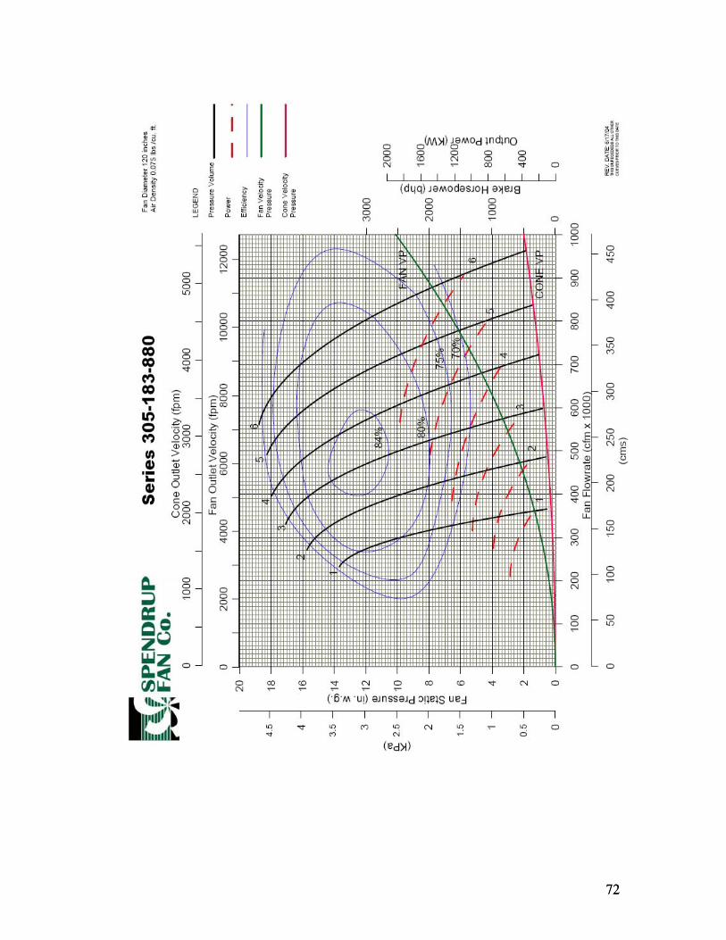
72
72

APPENDIX B: VENTILATION SCHEMATICS
73

Figure B.1 is the legend for the ventilation schematics. Figures B.2 – B.16 are the ventilation schematics of the mine for years 2 to 16. The schematic for year 1 was assumed to be the same as year 2, allowing a year for development before production mining begins. Table B.1 contains the corresponding VnetPC model branch input data for year 16. At this year, branches for all preceding years are included, and do not change over time.
Legend Node Numbering: 100’s, 500’s = Intakes 200’s, 400’s, 600’s = Returns 300’s, 700’s = Neutral R = Regulator --- = Stoppings Leakage
Figure B.1 – Ventilation Schematic Legend
74

Figure B.2 – Year 2 Ventilation Plan
75

Figure B.3 – Year 3 Ventilation Plan
76

Figure B.4 – Year 4 Ventilation Plan
77

Figure B.5 – Year 5 Ventilation Plan
78

Figure B.6 – Year 6 Ventilation Plan
79
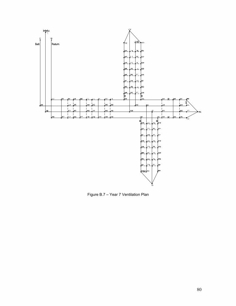
Figure B.7 – Year 7 Ventilation Plan
80

Figure B.8 – Year 8 Ventilation Plan
81
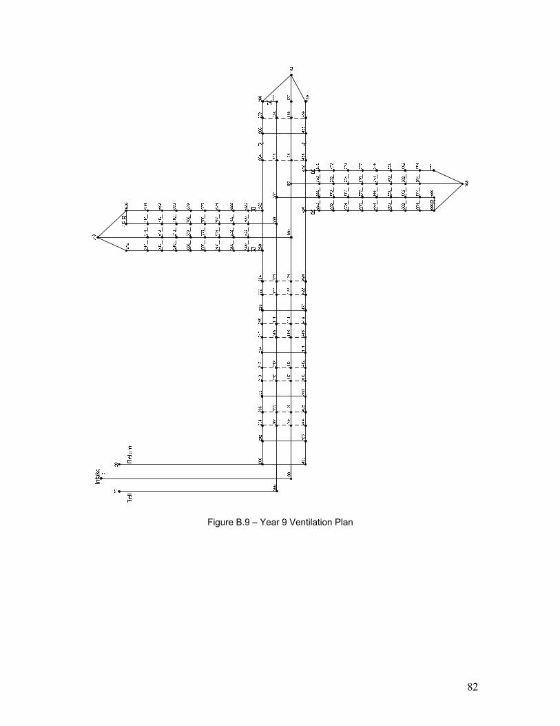
Figure B.9 – Year 9 Ventilation Plan
82

Figure B.10 – Year 10 Ventilation Plan
83

Figure B.11 – Year 11 Ventilation Plan
84

Figure B.12 – Year 12 Ventilation Plan
85

Figure B.13 – Year 13 Ventilation Plan
86

Figure B.14 – Year 14 Ventilation Plan
87

Figure B.15 – Year 15 Ventilation Plan
88

Figure B.16 – Year 16 Ventilation Plan
89

Table B.1 – Year 16 branch properties
From To Fqi TypeResistance (P.U.)
Resistance per Length (R/1000ft)
Length (ft)
Parallel Factor
Calculated Resistance (P.U.)
Branch Code
Surface State Description
10 100 R/L 0.0264 800 1 0.02112 Intake Intake Intake Shaft30 300 R/L 0.3033 2816 1 0.85409 Neutral Intake Belt Slope (Intake)
200 20 F R/L 0.0013 800 1 0.00104 Return Exhaust Exhaust Shaft100 104 R/L 0.0266 1000 3 0.00296 Intake Neither104 106 R/L 0.0266 1000 3 0.00296 Intake Neither106 110 R/L 0.0266 1000 3 0.00296 Intake Neither110 112 R/L 0.0266 1000 3 0.00296 Intake Neither112 116 R/L 0.0266 1000 3 0.00296 Intake Neither116 118 R/L 0.0266 1000 3 0.00296 Intake Neither118 122 R/L 0.0266 1000 3 0.00296 Intake Neither122 124 R/L 0.0266 1000 3 0.00296 Intake Neither124 128 R/L 0.0266 1000 3 0.00296 Intake Neither128 130 R/L 0.0266 1000 3 0.00296 Intake Neither130 134 R/L 0.0266 1000 3 0.00296 Intake Neither134 136 R/L 0.0266 1000 3 0.00296 Intake Neither136 140 R/L 0.0266 1000 3 0.00296 Intake Neither140 142 R/L 0.0266 1000 3 0.00296 Intake Neither142 146 R/L 0.0266 1000 3 0.00296 Intake Neither146 150 R/L 0.0266 700 3 0.00207 Intake Neither150 152 R/L 0.0266 500 3 0.00148 Intake Neither152 154 R/L 0.0266 300 3 0.00089 Intake Neither154 158 R/L 0.0266 1000 3 0.00296 Intake Neither158 160 R/L 0.0266 100 3 0.0003 Intake Neither160 162 Q R/L 0.0266 500 3 0.00148 Intake Neither Face 1162 260 R/L 0.0301 250 1 0.00752 Return Neither162 460 R/L 0.0301 250 1 0.00752 Return Neither300 304 R/L 0.0428 1000 1 0.0428 Neutral Neither304 306 R/L 0.0428 1000 1 0.0428 Neutral Neither306 310 R/L 0.0428 1000 1 0.0428 Neutral Neither310 312 R/L 0.0428 1000 1 0.0428 Neutral Neither312 316 R/L 0.0428 1000 1 0.0428 Neutral Neither316 318 R/L 0.0428 1000 1 0.0428 Neutral Neither318 322 R/L 0.0428 1000 1 0.0428 Neutral Neither322 324 R/L 0.0428 1000 1 0.0428 Neutral Neither324 328 R/L 0.0428 1000 1 0.0428 Neutral Neither328 330 R/L 0.0428 1000 1 0.0428 Neutral Neither330 334 R/L 0.0428 1000 1 0.0428 Neutral Neither334 336 R/L 0.0428 1000 1 0.0428 Neutral Neither336 340 R/L 0.0428 1000 1 0.0428 Neutral Neither340 342 R/L 0.0428 1000 1 0.0428 Neutral Neither342 346 R/L 0.0428 1000 1 0.0428 Neutral Neither346 350 R/L 0.0428 800 1 0.03424 Neutral Neither350 352 R/L 0.0428 500 1 0.0214 Neutral Neither352 354 R/L 0.0428 200 1 0.00856 Neutral Neither354 358 R/L 0.0428 1000 1 0.0428 Neutral Neither358 360 R/L 0.0428 100 1 0.00428 Neutral Neither360 260 Q R/L 0.0428 200 1 0.00856 Neutral Neither Belt 1200 202 R/L 0.0301 1000 2 0.00752 Return Neither202 204 R/L 0.0301 0 2 0 Return Neither204 206 R/L 0.0301 1000 2 0.00752 Return Neither206 208 R/L 0.0301 1000 2 0.00752 Return Neither208 210 R/L 0.0301 0 2 0 Return Neither210 212 R/L 0.0301 1000 2 0.00752 Return Neither212 214 R/L 0.0301 1000 2 0.00752 Return Neither214 216 R/L 0.0301 0 2 0 Return Neither216 218 R/L 0.0301 1000 2 0.00752 Return Neither218 220 R/L 0.0301 1000 2 0.00752 Return Neither
90

Table B.1 cont. – Year 16 Branch Properties
From To Fqi TypeResistance (P.U.)
Resistance per Length (R/1000ft)
Length (ft)
Parallel Factor
Calculated Resistance (P.U.)
Branch Code
Surface State Description
220 222 R/L 0.0301 0 2 0 Return Neither222 224 R/L 0.0301 1000 2 0.00752 Return Neither224 226 R/L 0.0301 1000 2 0.00752 Return Neither226 228 R/L 0.0301 0 2 0 Return Neither228 230 R/L 0.0301 1000 2 0.00752 Return Neither230 232 R/L 0.0301 1000 2 0.00752 Return Neither232 234 R/L 0.0301 0 2 0 Return Neither234 236 R/L 0.0301 1000 2 0.00752 Return Neither236 238 R/L 0.0301 1000 2 0.00752 Return Neither238 240 R/L 0.0301 0 2 0 Return Neither240 242 R/L 0.0301 1000 2 0.00752 Return Neither242 244 R/L 0.0301 1000 2 0.00752 Return Neither244 246 R/L 0.0301 0 2 0 Return Neither246 250 R/L 0.0301 500 2 0.00376 Return Neither250 252 R/L 0.0301 500 2 0.00376 Return Neither252 254 R/L 0.0301 500 2 0.00376 Return Neither254 256 R/L 0.0301 1000 2 0.00752 Return Neither From Face 1256 258 R/L 0.0301 500 2 0.00376 Return Neither258 260 R/L 0.0301 100 2 0.00075 Return Neither400 402 R/L 0.0301 1000 2 0.00752 Return Neither402 404 R/L 0.0301 0 2 0 Return Neither404 406 R/L 0.0301 1000 2 0.00752 Return Neither406 408 R/L 0.0301 1000 2 0.00752 Return Neither408 410 R/L 0.0301 0 2 0 Return Neither410 412 R/L 0.0301 1000 2 0.00752 Return Neither412 414 R/L 0.0301 1000 2 0.00752 Return Neither414 416 R/L 0.0301 0 2 0 Return Neither416 418 R/L 0.0301 1000 2 0.00752 Return Neither418 420 R/L 0.0301 1000 2 0.00752 Return Neither420 422 R/L 0.0301 0 2 0 Return Neither422 424 R/L 0.0301 1000 2 0.00752 Return Neither424 426 R/L 0.0301 1000 2 0.00752 Return Neither426 428 R/L 0.0301 0 2 0 Return Neither428 430 R/L 0.0301 1000 2 0.00752 Return Neither430 432 R/L 0.0301 1000 2 0.00752 Return Neither432 434 R/L 0.0301 0 2 0 Return Neither434 436 R/L 0.0301 1000 2 0.00752 Return Neither436 438 R/L 0.0301 1000 2 0.00752 Return Neither438 440 R/L 0.0301 0 2 0 Return Neither440 442 R/L 0.0301 1000 2 0.00752 Return Neither442 444 R/L 0.0301 1000 2 0.00752 Return Neither444 446 R/L 0.0301 0 2 0 Return Neither446 450 R/L 0.0301 500 2 0.00376 Return Neither450 452 R/L 0.0301 500 2 0.00376 Return Neither452 454 R/L 0.0301 500 2 0.00376 Return Neither454 456 R/L 0.0301 1000 2 0.00752 Return Neither From Face 1456 458 R/L 0.0301 500 2 0.00376 Return Neither458 460 R/L 0.0301 100 2 0.00075 Return Neither200 400 R/L 0.0301 700 1 0.02107 Return Neither202 402 R/L 0.0301 700 1 0.02107 Return Neither208 408 R/L 0.0301 700 1 0.02107 Return Neither214 414 R/L 0.0301 700 1 0.02107 Return Neither220 420 R/L 0.0301 700 1 0.02107 Return Neither226 426 R/L 0.0301 700 1 0.02107 Return Neither
91

Table B.1 cont. – Year 16 Branch Properties
From To Fqi TypeResistance (P.U.)
Resistance per Length (R/1000ft)
Length (ft)
Parallel Factor
Calculated Resistance (P.U.)
Branch Code
Surface State Description
232 432 R/L 0.0301 700 1 0.02107 Return Neither238 438 R/L 0.0301 700 1 0.02107 Return Neither244 444 R/L 0.0301 700 1 0.02107 Return Neither256 456 R/L 0.0301 700 1 0.02107 Return Neither204 304 R 22.5 1 22.5 Default Neither304 104 R 22.5 1 22.5 Default Neither104 404 R 22.5 1 22.5 Default Neither254 354 R 22.5 1 22.5 Default Neither354 154 R 22.5 1 22.5 Default Neither154 454 R 22.5 1 22.5 Default Neither258 358 R 22.5 1 22.5 Default Neither358 158 R 22.5 1 22.5 Default Neither158 458 R 22.5 1 22.5 Default Neither206 306 R 22.5 1 22.5 Default Neither306 106 R 22.5 1 22.5 Default Neither106 406 R 22.5 1 22.5 Default Neither210 310 R 22.5 1 22.5 Default Neither310 110 R 22.5 1 22.5 Default Neither110 410 R 22.5 1 22.5 Default Neither212 312 R 22.5 1 22.5 Default Neither312 112 R 22.5 1 22.5 Default Neither112 412 R 22.5 1 22.5 Default Neither216 316 R 22.5 1 22.5 Default Neither316 116 R 22.5 1 22.5 Default Neither116 416 R 22.5 1 22.5 Default Neither218 318 R 22.5 1 22.5 Default Neither318 118 R 22.5 1 22.5 Default Neither118 418 R 22.5 1 22.5 Default Neither222 322 R 22.5 1 22.5 Default Neither322 122 R 22.5 1 22.5 Default Neither122 422 R 22.5 1 22.5 Default Neither224 324 R 22.5 1 22.5 Default Neither324 124 R 22.5 1 22.5 Default Neither124 424 R 22.5 1 22.5 Default Neither228 328 R 22.5 1 22.5 Default Neither328 128 R 22.5 1 22.5 Default Neither128 428 R 22.5 1 22.5 Default Neither230 330 R 22.5 1 22.5 Default Neither330 130 R 22.5 1 22.5 Default Neither130 430 R 22.5 1 22.5 Default Neither234 334 R 22.5 1 22.5 Default Neither334 134 R 22.5 1 22.5 Default Neither134 434 R 22.5 1 22.5 Default Neither236 336 R 22.5 1 22.5 Default Neither336 136 R 22.5 1 22.5 Default Neither136 436 R 22.5 1 22.5 Default Neither240 340 R 22.5 1 22.5 Default Neither340 140 R 22.5 1 22.5 Default Neither140 440 R 22.5 1 22.5 Default Neither242 342 R 22.5 1 22.5 Default Neither342 142 R 22.5 1 22.5 Default Neither142 442 R 22.5 1 22.5 Default Neither246 346 R 22.5 1 22.5 Default Neither346 146 R 22.5 1 22.5 Default Neither
92
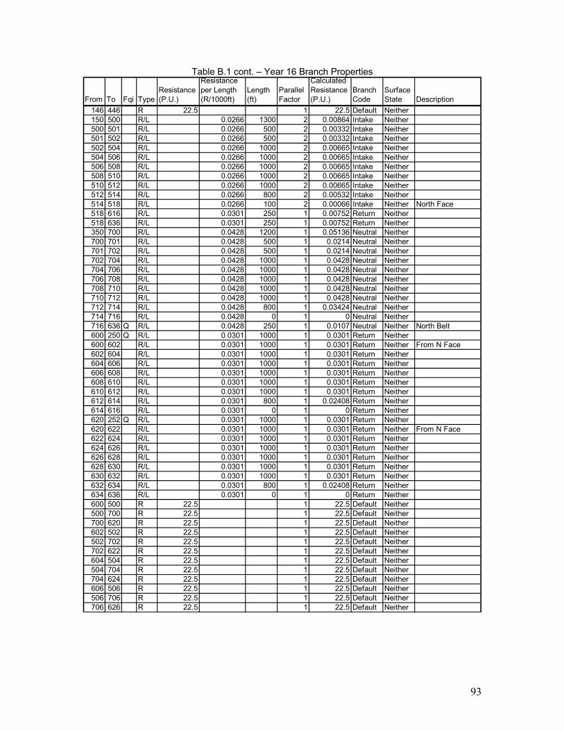
Table B.1 cont. – Year 16 Branch Properties
From To Fqi TypeResistance (P.U.)
Resistance per Length (R/1000ft)
Length (ft)
Parallel Factor
Calculated Resistance (P.U.)
Branch Code
Surface State Description
146 446 R 22.5 1 22.5 Default Neither150 500 R/L 0.0266 1300 2 0.00864 Intake Neither500 501 R/L 0.0266 500 2 0.00332 Intake Neither501 502 R/L 0.0266 500 2 0.00332 Intake Neither502 504 R/L 0.0266 1000 2 0.00665 Intake Neither504 506 R/L 0.0266 1000 2 0.00665 Intake Neither506 508 R/L 0.0266 1000 2 0.00665 Intake Neither508 510 R/L 0.0266 1000 2 0.00665 Intake Neither510 512 R/L 0.0266 1000 2 0.00665 Intake Neither512 514 R/L 0.0266 800 2 0.00532 Intake Neither514 518 R/L 0.0266 100 2 0.00066 Intake Neither North Face518 616 R/L 0.0301 250 1 0.00752 Return Neither518 636 R/L 0.0301 250 1 0.00752 Return Neither350 700 R/L 0.0428 1200 1 0.05136 Neutral Neither700 701 R/L 0.0428 500 1 0.0214 Neutral Neither701 702 R/L 0.0428 500 1 0.0214 Neutral Neither702 704 R/L 0.0428 1000 1 0.0428 Neutral Neither704 706 R/L 0.0428 1000 1 0.0428 Neutral Neither706 708 R/L 0.0428 1000 1 0.0428 Neutral Neither708 710 R/L 0.0428 1000 1 0.0428 Neutral Neither710 712 R/L 0.0428 1000 1 0.0428 Neutral Neither712 714 R/L 0.0428 800 1 0.03424 Neutral Neither714 716 R/L 0.0428 0 1 0 Neutral Neither716 636 Q R/L 0.0428 250 1 0.0107 Neutral Neither North Belt600 250 Q R/L 0.0301 1000 1 0.0301 Return Neither600 602 R/L 0.0301 1000 1 0.0301 Return Neither From N Face602 604 R/L 0.0301 1000 1 0.0301 Return Neither604 606 R/L 0.0301 1000 1 0.0301 Return Neither606 608 R/L 0.0301 1000 1 0.0301 Return Neither608 610 R/L 0.0301 1000 1 0.0301 Return Neither610 612 R/L 0.0301 1000 1 0.0301 Return Neither612 614 R/L 0.0301 800 1 0.02408 Return Neither614 616 R/L 0.0301 0 1 0 Return Neither620 252 Q R/L 0.0301 1000 1 0.0301 Return Neither620 622 R/L 0.0301 1000 1 0.0301 Return Neither From N Face622 624 R/L 0.0301 1000 1 0.0301 Return Neither624 626 R/L 0.0301 1000 1 0.0301 Return Neither626 628 R/L 0.0301 1000 1 0.0301 Return Neither628 630 R/L 0.0301 1000 1 0.0301 Return Neither630 632 R/L 0.0301 1000 1 0.0301 Return Neither632 634 R/L 0.0301 800 1 0.02408 Return Neither634 636 R/L 0.0301 0 1 0 Return Neither600 500 R 22.5 1 22.5 Default Neither500 700 R 22.5 1 22.5 Default Neither700 620 R 22.5 1 22.5 Default Neither602 502 R 22.5 1 22.5 Default Neither502 702 R 22.5 1 22.5 Default Neither702 622 R 22.5 1 22.5 Default Neither604 504 R 22.5 1 22.5 Default Neither504 704 R 22.5 1 22.5 Default Neither704 624 R 22.5 1 22.5 Default Neither606 506 R 22.5 1 22.5 Default Neither506 706 R 22.5 1 22.5 Default Neither706 626 R 22.5 1 22.5 Default Neither
93

Table B.1 cont. – Year 16 Branch Properties
From To Fqi TypeResistance (P.U.)
Resistance per Length (R/1000ft)
Length (ft)
Parallel Factor
Calculated Resistance (P.U.)
Branch Code
Surface State Description
608 508 R 22.5 1 22.5 Default Neither508 708 R 22.5 1 22.5 Default Neither708 628 R 22.5 1 22.5 Default Neither610 510 R 22.5 1 22.5 Default Neither510 710 R 22.5 1 22.5 Default Neither710 630 R 22.5 1 22.5 Default Neither612 512 R 22.5 1 22.5 Default Neither512 712 R 22.5 1 22.5 Default Neither712 632 R 22.5 1 22.5 Default Neither614 514 R 35.2 1 35.2 Default Neither514 714 R 35.2 1 35.2 Default Neither714 634 R 35.2 1 35.2 Default Neither152 550 R/L 0.0266 1000 2 0.00665 Intake Neither550 551 R/L 0.0266 500 2 0.00332 Intake Neither551 552 R/L 0.0266 500 2 0.00332 Intake Neither552 554 R/L 0.0266 1000 2 0.00665 Intake Neither554 556 R/L 0.0266 1000 2 0.00665 Intake Neither556 558 R/L 0.0266 1000 2 0.00665 Intake Neither558 560 R/L 0.0266 1000 2 0.00665 Intake Neither560 562 R/L 0.0266 1000 2 0.00665 Intake Neither562 564 R/L 0.0266 800 2 0.00532 Intake Neither564 568 R/L 0.0266 100 2 0.00066 Intake Neither South Face568 666 R/L 0.0301 250 1 0.00752 Return Neither568 686 R/L 0.0301 250 1 0.00752 Return Neither352 750 R/L 0.0428 1000 1 0.0428 Neutral Neither750 751 R/L 0.0428 500 1 0.0214 Neutral Neither751 752 R/L 0.0428 500 1 0.0214 Neutral Neither752 754 R/L 0.0428 1000 1 0.0428 Neutral Neither754 756 R/L 0.0428 1000 1 0.0428 Neutral Neither756 758 R/L 0.0428 1000 1 0.0428 Neutral Neither758 760 R/L 0.0428 1000 1 0.0428 Neutral Neither760 762 R/L 0.0428 1000 1 0.0428 Neutral Neither762 764 R/L 0.0428 800 1 0.03424 Neutral Neither764 766 R/L 0.0428 0 1 0 Neutral Neither766 666 Q R/L 0.0301 250 1 0.00752 Return Neither South Belt650 450 Q R/L 0.0301 1000 1 0.0301 Return Neither From S Face650 652 R/L 0.0301 1000 1 0.0301 Return Neither652 654 R/L 0.0301 1000 1 0.0301 Return Neither654 656 R/L 0.0301 1000 1 0.0301 Return Neither656 658 R/L 0.0301 1000 1 0.0301 Return Neither658 660 R/L 0.0301 1000 1 0.0301 Return Neither660 662 R/L 0.0301 1000 1 0.0301 Return Neither662 664 R/L 0.0301 800 1 0.02408 Return Neither664 666 R/L 0.0301 0 1 0 Return Neither670 450 Q R/L 0.0301 1000 1 0.0301 Return Neither From S Face670 672 R/L 0.0301 1000 1 0.0301 Return Neither672 674 R/L 0.0301 1000 1 0.0301 Return Neither674 676 R/L 0.0301 1000 1 0.0301 Return Neither676 678 R/L 0.0301 1000 1 0.0301 Return Neither678 680 R/L 0.0301 1000 1 0.0301 Return Neither680 682 R/L 0.0301 1000 1 0.0301 Return Neither682 684 R/L 0.0301 800 1 0.02408 Return Neither684 686 R/L 0.0301 0 1 0 Return Neither650 750 R 22.5 1 22.5 Default Neither
94

Table B.1 cont. – Year 16 Branch Properties
From To Fqi TypeResistance (P.U.)
Resistance per Length (R/1000ft)
Length (ft)
Parallel Factor
Calculated Resistance (P.U.)
Branch Code
Surface State Description
750 550 R 22.5 1 22.5 Default Neither550 670 R 22.5 1 22.5 Default Neither652 752 R 22.5 1 22.5 Default Neither752 552 R 22.5 1 22.5 Default Neither552 672 R 22.5 1 22.5 Default Neither654 754 R 22.5 1 22.5 Default Neither754 554 R 22.5 1 22.5 Default Neither554 674 R 22.5 1 22.5 Default Neither656 756 R 22.5 1 22.5 Default Neither756 556 R 22.5 1 22.5 Default Neither556 676 R 22.5 1 22.5 Default Neither658 758 R 22.5 1 22.5 Default Neither758 558 R 22.5 1 22.5 Default Neither558 678 R 22.5 1 22.5 Default Neither660 760 R 22.5 1 22.5 Default Neither760 560 R 22.5 1 22.5 Default Neither560 680 R 22.5 1 22.5 Default Neither662 762 R 22.5 1 22.5 Default Neither762 562 R 22.5 1 22.5 Default Neither562 682 R 22.5 1 22.5 Default Neither664 764 R 35.2 1 35.2 Default Neither764 564 R 35.2 1 35.2 Default Neither564 684 R 35.2 1 35.2 Default Neither
95

APPENDIX C: EXCEL PROGRAM FOR SOLVING REDUCED SPEEDS
96

Figure C.1 is the first page in the Excel workbook. Clicking the ‘Start’ button runs a Visual Basic for Applications (VBA) macro that opens the form in Figure C.2.
Click the 'Start' button to run the speed calculator
Notes: Solver must be installed in Excel, and marcos enabled. - To enable macros, select 'Security...' from the Tools-->Macro menu- To install solver, go to the Tools-->Add-ins menu and check the box next to "Solver Add-in" - If you receive a "Compile Error: Can't find project or library" message, view the help worksheet tab below for instructions.
Start
Figure C.1 – Excel Start Page
Figure C.2 – Program’s primary screen
This screen lists the steps necessary to solve reduced speed fan curves, numbered 1 to 4. Fan curve data and operating point data are required inputs. Clicking these buttons opens the forms to input this information, Figures C.3 and C.4, respectively. The program allows for up to six fan curves to be inputted, and up to 20 operating points. Fan curve data required includes digitized points of both the fan curve and power curve.
97

Figure C.3 – Fan curve input
98

Figure C.4 – Operating point input
Once the fan curves and operating points are inputted into the forms, and the values saved, calculations can be performed. The third step is to select a fan curve to use for analysis. This requires user knowledge of mine ventilation practices to make the appropriate choice. The last step is to find the reduced speed information. Referring to step 4 shown in Figure C.2, this can be done for one operating point at a time, or for all operating points sequentially. The resulting output spreadsheet of results in shown in Figure C.5.
99

Table C.1 – Spreadsheet output: Summary of results Summary of Yearly Fan Operating PointsAnd Reduced Speed and Pitch Settings
Operating Point
Year Speed Pitch Setting Q, kcfm H, in. WG Air Power, hp Brake Power, hpFan Efficiency,
%1 350 6 219 1.70 58 77 76%2 350 6 219 1.70 58 77 76%3 375 6 231 2.02 73 96 76%4 401 6 244 2.37 91 119 77%5 426 6 257 2.73 111 144 77%6 450 6 269 3.08 131 171 76%7 478 6 285 3.53 158 206 77%8 514 6 305 4.13 198 257 77%9 550 6 324 4.77 244 317 77%10 592 6 348 5.55 304 397 77%11 628 6 368 6.29 364 475 77%12 670 6 391 7.16 442 579 76%13 712 6 415 8.14 532 695 77%14 766 6 446 9.44 663 866 77%15 815 6 474 10.74 803 1044 77%16 876 6 509 12.40 994 1299 77%
100

APPENDIX D: MOTOR MODEL
101

Motor Performance Data
Figure D.1 – Motor performance data, page 1
102

Figure D.2 – Motor performance data, page 2
103

Motor modeling program m-file content (induction.m): clc; clear; clf; % input motor data % constants pi = 4.0*atan(1.0); % Number of Poles np=8; % Impedance Base zb=15.465; % frequency of operation (Hz) n=input('Sync. Speed, rpm : '); % Use to input speed in rpm wsm=n*pi/30; %wsm=input('Speed:'); % Use to input speed in rad/sec f=wsm*np/(4*pi); %f=input('Freq:'); % Use to enter frequency directly %wsm = 4*pi*f/np; % stator r1 = 0.0051; x1 = 0.07227; z1 = zb*(r1+i*x1*f/60); % rotor r2 = zb*0.0251; x2 = zb*0.07227; % magnetizing branch (series form) rm = 0.00; xm = 0.4000; zm = zb*(rm + i*xm*f/60); % terminal voltage (line-to-neutral) vt1=69.333*f; % 69.33 is constant derived from rated speed and freq vt = vt1/sqrt(3) + i*0.0000; % calculate thevenin equivalent vth = vt*zm/(z1+zm); vthm = abs(vth); zth = z1*zm/(z1+zm); rth = real(zth); xth = imag(zth); % load is considered of the form TL = kl*w**2 kl=input('k value: '); % Use if k is known %T=input('Torque Required : '); % Use if T is directly inputted %kl=T/wsm^2; % motor-load moment of inertia J = 5000; dt = 0.05; w0 = 0.0; dw=0; % final time of simulation in seconds tf = 60; ns = tf/dt + 1; % total number of steps % initiate simulation cycle for k =1: ns;
104

if k == 1 w(k) = w0; else w(k) = w(k-1) + dw; nm(k)=w(k)*30/pi; end time(k) = dt * (k-1); s = (wsm-w(k))/wsm; z2 = r2/s + i*x2*f/60; tem(k) = 3*vthm^2*r2/(s*wsm*((rth+r2/s)^2 + (xth+x2)^2)); tl(k) = kl*w(k)^2; ta(k) = tem(k) - tl(k); acc(k) = ta(k)/J; dw = acc(k)*dt; i2(k)=vth/(zth+z2); i1(k) = i2(k)*(z2+zm)/zm; i1m(k) = abs(i1(k)); ani1(k)=angle(i1(k)); pin(k)=3*vt*i1m(k)*cos(ani1(k)); pout(k)=tem(k)*w(k); eff(k)=pout(k)/pin(k); end plot(time, tem) fprintf('\nMechanical Speed = %3.f rpm \n',w(1000)*30/pi) fprintf('Torque = %5.f Nm \n',tem(1000)) fprintf('Efficiency = %3.f percent \n',eff(1000)*100)
105

Figures D.3 and D.4 show the motor model command and plot windows showing input and output.
Figure D.3 – Matlab command window input and output text
Figure D.4 – Output plot of torque versus time
106

APPENDIX E: ABB DRIVE SPECIFICATIONS
107

108

109

110

111

112

113