a method for estimating intensity of a poisson process

UNLV Retrospective Theses & Dissertations

1-1-2007

A method for estimating intensity of a Poisson process A method for estimating intensity of a Poisson process

Sandhya Gunti University of Nevada, Las Vegas

Follow this and additional works at: https://digitalscholarship.unlv.edu/rtds

Repository Citation Repository Citation Gunti, Sandhya, "A method for estimating intensity of a Poisson process" (2007). UNLV Retrospective Theses & Dissertations. 2112. http://dx.doi.org/10.25669/nv5n-bfbk

This Thesis is protected by copyright and/or related rights. It has been brought to you by Digital Scholarship@UNLV with permission from the rights-holder(s). You are free to use this Thesis in any way that is permitted by the copyright and related rights legislation that applies to your use. For other uses you need to obtain permission from the rights-holder(s) directly, unless additional rights are indicated by a Creative Commons license in the record and/or on the work itself. This Thesis has been accepted for inclusion in UNLV Retrospective Theses & Dissertations by an authorized administrator of Digital Scholarship@UNLV. For more information, please contact [email protected].

http://library.unlv.edu/

http://library.unlv.edu/

https://digitalscholarship.unlv.edu/rtds

https://digitalscholarship.unlv.edu/rtds?utm_source=digitalscholarship.unlv.edu%2Frtds%2F2112&utm_medium=PDF&utm_campaign=PDFCoverPages

http://dx.doi.org/10.25669/nv5n-bfbk

mailto:[email protected]

A METHOD FOR ESTIMATING INTENSITY OF A POISSON PROCESS

by

Sandhya Gunti

Bachelor of Engineering Osmania University, Andhra Pradesh, India

April 2003

A thesis submitted in partial fulfillment of the requirements for the

Master of Science Degree in Mathematical Sciences Department of Mathematical Sciences

College of Sciences

Graduate College University of Nevada, Las Vegas

May 2007

Reproduced with permission of the copyright owner. Further reproduction prohibited without permission.

UMI Number: 1443760

INFORMATION TO USERS

The quality of this reproduction is dependent upon the quality of the copy

submitted. Broken or indistinct print, colored or poor quality illustrations and

photographs, print bleed-through, substandard margins, and improper

alignment can adversely affect reproduction.

In the unlikely event that the author did not send a complete manuscript

and there are missing pages, these will be noted. Also, if unauthorized

copyright material had to be removed, a note will indicate the deletion.

UMIUMI Microform 1443760

Copyright 2007 by ProQuest Information and Learning Company.

All rights reserved. This microform edition is protected against

unauthorized copying under Title 17, United States Code.

ProQuest Information and Learning Company 300 North Zeeb Road

P.O. Box 1346 Ann Arbor, Ml 48106-1346


UNIV Thesis ApprovalThe Graduate College University of Nevada, Las Vegas

March 2 , 20 07

The Thesis prepared by

Sandhya G un ti

Entitled

A M ethod For E s t im a t in g I n t e n s i t y Of A P o is s o n P r o c e s s

is approved in partial fulfillment of the requirements for the degree of

M aster o f S c ie n c e in M a th e m a tic a l S c ie n c e s

Exam ination C om m ittee M em ber

Exam ination C om m ittee M em ber

^ I u lZ ^ _________G raduate College F acidty R epresentative

Exam ination C om m ittee Chair

Dean o f the G raduate College

11


ABSTRACT

A Method for Estimating Intensity of a Poisson Process

by

Sandhya Gunti

Dr. Chih-Hsiang Ho, Examination Committee Chair Professor of Mathematical Sciences

University of Nevada, Las Vegas

Motivated by its vast applications, we investigate ways to estimate the intensity of

a Poisson process. Much of the work on modeling and analysis of repairable systems is

based on the assumption of a special type of nonhomogeneous Poisson process (NHPP)

known as Weibull process or Power-law process. In this thesis, we link the traditional

homogeneous and nonhomogeneous Poisson processes to the classical time series via a

sequence of the empirical recurrence rates (ERR), calculated at equally spaced intervals

of time. We consider a computationally simple algorithm to calculate the total area and

also the area for the last ten recurrence rates under the ERR curve. We conclude that the

mean function of an NHPP can be estimated from the ERR values. In addition, we argue

by simulation, that the algorithm can be implemented to forecast NHPP observations with

various forms of intensity function. A correction factor is defined based on the overall

trend of the targeted point process.

Ill


TABLE OF CONTENTS

ABSTRACT.............................................................................................................................. iii

LIST OF TABLES................................................................................................... vi

ACKNOWLEDGEMENTS............................................. vii

CHAPTERl INTRODUCTION............................ 11.1 Basic Theory of Point Process................................................................................ 11.2 Poisson Process......................................................................................................... 41.3 Objective of the Thesis..............................................................................................5

CHAPTER2 POWER LAW PROCESS..............................................................................62.1 Analysis of NHPP.................................................................................. 62.2 Statistical Inferences ...................................................................... 14

CHAPTER3 EMPIRICAL RECURRENCE RATES TIME SERIES............................ 183.1 Relationship between Mean and Intensity Functions of NHPP...........................183.2 The Empirical Recurrence Rates(ERR)............................... 203.3 Area Under ERR Plots............................................................................................213.4 Methodology............................................................................................................22

CHAPTER4 RESULTS...................................................................................................... 254.1 Summary for jS = 0.5,1,2 .......................................................................................264.2 Summary for Increasing Step Intensity................ 274.3 Summary for Decreasing Step Intensity................................................................ 284.4 Description of the Simulation Results................................................................... 29

CHAPTER5 APPLICATIONS .................................................................................... 315.1 Mining D ata............... 315.2 ERR Plotting of Mining Data...................................................................................325.3 Predicting the Mean Function....................................................................... 335.4 Summary of the Simulation Results for Mining Data.......................................... 35

CHAPTER6 CONCLUSIONS AND FUTURE WORK................................................. 366.1 Conclusions.................................... 366.2 Future W ork............................................................................................................. 37

CHAPTER7 R-ROGRAMS................................................................................................387.1 Program for = 0.5,1,2 ..........................................................................................38

iv


7.2 Program for Increasing Step Intensity................ 397.3 Program for Decreasing Step Intensity.................................................................407.4 Program for Mining Data....................................................................................... 41

REFERENCES .............................................................................................................. 43

VITA................................................................................................. 45


LIST OF TABLES

Table 4.1 Results for NHPP with p = 0.5,1,2...............................................................26Table 4.2 Results for NHPP with X(t) = 3, for 0 < t < t & X(t) = 1, for t < t < oo 27Table 4.3 Results for NHPP with X(t) = 1, for 0 < t < t & X(t) = 3, for t < t < oo 28Table 5.1 Time Intervals in Days between Explosions in Mines, Involving 10 Men

Killed, from 6 December 1875 to 29 May 1951..........................................32Table 5.2 Results for the First 62 years.......................................................................... 34Table 5.3 Results for the Last 10 years, with C.F = 0.7219992................................... 35

VI


ACKNOWLEDGEMENTS

I would like to dedicate this thesis to my parents, my husband, Goverdhan

Gajjala, and friends whose love, support and understanding have always motivated me to

strive for excellence.

I would like to sincerely and wholeheartedly thank Dr. Chih-Hsiang Ho for his

guidance and kindness throughout this work. His patience as an advisor, boundless

energy while teaching, promptness while reviewing all my writing, and passion for

research are to be commended and worth emulating. I owe most of this work to him.

My deeply indebtedness also give to respectable committee members. Dr. Ananda,

Dr. Cho and Dr. Qian, for their positive inputs and mentoring during my graduate studies.

VII


CHAPTER 1

INTRODUCTION

Reliability is the ability of a system or component to perform its required

functions under stated conditions for a specified period of time and it plays a key role in

developing quality products and in enhancing competitiveness. Quality is a snapshot at

the start of life and reliability is a motion picture of the day-by-day operation. Time zero

defects are manufacturing mistakes that escaped final test. The additional defects that

appear over time are "reliability defects" or reliability fallout. Much of the theory of

reliability deals with nonrepairable systems or devices and it emphasizes the study of life

time models. The main distinction between nonrepairable and repairable systems is that

the former can fail only once, and Weibull distribution serves as a life time model for it

where as the later is one which can be repaired and can be placed back in service. A

repairable system is often modeled by a point process.

1.1 Basic Theory of Point Process

A point process is a stochastic model that describes the occurrences of events in

time. These occurrences are thought as points on the time axis. In general the times

between failures are neither independent nor identically distributed. Let X( t ) be a random

variable that denotes the number of failures in the interval (0,t] and X is called the

counting random variable.


The probability that a unit survives beyond time is called the reliability at

timetq, and the reliability function, is defined as

^(^o) = T [ r > t J = l-F ( to ) ,

where F{t) gives the probability that a randomly selected unit will fail by time t.

In biomedical applications the term “survival function” is also used. The probability

density fimction (pdf) is defined to be the derivative of the cdf, provided the derivative

exits. That is,

f ( x ) - — F ( x ) - —— S(x) ax ax

Life testing model can be characterized in terms of a number of different concepts. The

hazard function ( HF ) is defined by

In actuarial science h{t) is known as the “force of mortality,” and in extreme-value theory

h{t) is called the “intensity function.” This concept is often referred to as the “failure

rate.”

1.1.1 Mean function of a point process

The mean function of a point process is defined to be the expectation

m(Q = E(;ir(0)

Thus m{t) is the expected number of failures through time t, and so it must be a non

decreasing function. Because X(t ) is a non-decreasing step function, it is clear that the

mean function must be non-decreasing.


1.1.2 Rate of occurrence of failures (ROCOF)

When m{t) is differentiable we define ROCOF as

at

This can be interpreted as the instantaneous rate of change in the expected number of

failures.

1.1.3 Intensity function

Let X(t) denote the number of occurrences in the interval [0 ,t], and = P [n

occurrences in an interval (0,t)]. The intensity function of a point process (Rigdon and

Basu, 2000) is

Roughly speaking, the intensity function is the probability of failure in a small

interval divided by the length of the interval. Thus, there will be many failures over

intervals on which A(t) is large, and fewer failures over intervals on which X{t) is small.

It is instructive to compare the definitions of the hazard function and intensity function.

The hazard function is the limit of a conditional probability that the one and only one

failure will occur in a small interval, divided by the length of the interval. This

probability is conditioned on survival to the beginning of the interval. The intensity

function is the unconditional probability of a failure in a small interval divided by the

length of the interval (Rigdon and Basu, 2000). Clearly the intensity and ROCOF

functions are the same provided that simultaneous failures cannot occur, i.e., when the

mean function m{t) is not discontinuous.


1.2 Poisson Process

A point process X (t) is said to be a Poisson process if

1. Y(0) = 0

2. > 0} has independent increments.

3. F[X(t + h )-X (t) = 1] = À(/)/? + o(h), where the function, X is called the

intensity function of the Poisson Process.

4. P[Xit + h ) - X { t )> 2] ^ o{ h )

1.2.1 Homogeneous Poisson Process (HPP)

The HPP is a Poisson process with constant intensity function. In terms of a

repairable system, this implies that the system is neither improving nor wearing out with

age, but rather is maintaining a constant intensity of failure.

1.2.2 Nonhomogeneous Poisson Process (NHPP)

In this thesis we focus on arrival (counting) processes, and more particularly,

arrival processes that can be classified as nonstationary point processes. For such

processes we are able to observe each arrival time exactly, and in general the arrival

intensity (rate) changes over time.

Then P { X ( t ) = n ) = - — ,« > 0, where m(t)= |A(5)ife.

Under certain assumptions a nonstationary arrival process can be represented as

NHPP (Cinlar, 1975). Using NHPPs, we can accurately represent a large class of arrival

processes encountered in practice.


1.2.3 Weibull process

The special type of NHPP known as a Weibull process which is also known in the

literature as a Power Law process. The name Weibull process derives primarily from the

resemblance of the intensity function of the process to the hazard function o f a Weibull

distribution. In particular the intensity function has the form

tG

X{t)

[ he mean value function of a Weibull function of a Weibull process has the form

m ( 0 = E m 0 ] = { / g f

with scale parameter 6 >0 and shape parameter p >0.

1.3 Objective of the Thesis

Estimating the intensity of the failures is the important task which is the main

objective of the thesis. To begin with, we try to establish the relation between HPP and

NHPP, and the statistical inferences of Power law Process as shown in chapter 2. From

chapter 3, we try to get the mean function from the area under the ERR plot by defining a

correction factor. From the results in chapter 4, it will be proved that the correction factor

can be used improve predicting the mean function of the coming failures and it will be

applied to the mining accidents data in the chapter 5. The algorithms used for simulation

are given in chapter 7.


CHAPTER 2

POWER-LAW PROCESS

The Power law process has the intensity function of the form

,0,

The p parameter affects how the system deteriorates or improves over time. If /3 > 1

then the intensity function X(t) is increasing, and the failures tend to occur more

frequently, if < 1, then X(t) is decreasing, and the system is improving. Finally if = 1,

then the power law process reduces to the simpler HPP with intensity 1/0. There are

several reasons why the power law process is widely used model for repairable systems.

In the coming sections we link the traditional HPP with Weibull process and finally prove

that Weibull process is a special case of NHPP.

2.1 Analysis of NHPP

2.1.1 Joint pdf of HPP with intensity A = 1

Theorem 2.1: Let the random variables Z, < <... < are distributed as the first n

successive times of an HPP with intensity X = l

If we let Zg = 0, it follows from basic properties of an HPP that the differences

Z, -Z^_, for i = !,...,« are independent exponential random variables with mean =1.


It follows that the joint probability density fimction of is,

/(Z i,Z 2 ,.. .,Z J = exp (-z„),if 0< Z , <Z 2 < ...<Z„ < 0 0 .

Proof: Let Zj,Z 2 ,...,Z„ denote the failure times in an HPP, and let X . —Z^-Z^_^

(where Zg = 0 ) be the times between failures. Deriving the joint pdf of

Z,, Z2 ,..., Z„ by using the following relationship

; ^ 2 ; ^ 3 ; ^ y i ( ^ 1 ) y 2 ( ^ 2 \ \ I ’ - ^ 2 ’ ^ n - 1 )

where 0 < z, < Z2 <... < z„. The survival function for Z, is

^(z,) = f (Z ,> z ,)

= P(V (0,zJ = 0)

= exp |-J^ 'l< irj

= exp(-Azj), z, >0

The pdf of Z, is thus

/ ( z , ) = -^ ',(z j

= Aexp(-Zz,), z, >0

The conditional survival function of Z 2 given Z, =z, is

^2(^2kl) = (^2 > ^2 l^ ,)

= f(V(z„Z2] = 0)

= exp|-^"A<ixj

= exp[Z(z2 - z ,) ] , Z2 > Z] > 0

The conditional pdf of Z 2 given Z, = Zj is thus


| Z , ) = - ; ^ ^ 2 ( Z 2 | z , ) az^

= A exp[-A(z2 - z,)], Z2 > Zj > 0

Because of the independent increments property, the conditional pdf of Z3 given Z, = z,

and Z2 = Z2 is independent o fz ,. The conditional survival function for Z3 is therefore

■3 ( ^ 3 I ^1 5^2 ) “ T(Z3 > Z3 I Zj = Z],Z2 = Z2 )

= P ( Z 3 > Z 3 | Z 2 = Z 2 )

= P ( V ( Z 2 , Z 3 ] = 0 )

= e x p |- £ ' Acfrj

=exp[-A(z3 -Z 2 )], Z3 > Zj > 0

In general, we have

1 = -^exp[-A(z, -z^_j)], z > z _j > 0

The j oint pdf of Zj, Z j,..., Z„ is thus

/(z ,,Z 2 ,Z3 ....z„)=[Aexp(-Azj)]{ Aexp[-A(z2 -z ,)] }{Aexp[-A(z3 -Z 2 ) ] }

x...x(Aexp[-A(z„-z„_,)]}

= A” exp(-Az„) , z„ > z„_, >... > Z2 > Zj > 0

In our case A = 1, so

/(Z ,,Z 2 ,...,Z„) = exp(-z„).


2.1.2 Joint distribution of Weibull process using HPP

Theorem 2.2: Suppose m{t) is continuous. If Z, = for i = then the random

variables Z, < Z <... < Z„ are distributed as the first n successive times of an HPP with

intensity A = 1

In the case of a Weibull process, m{t) = , which means that 7] =

This transformation yields the joint probability density function of 7j,7 ,...,7%, namely

for 0 < t, < < ...t„ < 0 0 .

Proof: Given = is continuous

Let T. = m(Z,) & Z, = m{Tf)

Therefore Z, =

=>T =Z ./^0

Let us derive the joint using distribution using Jacobian under transformation

Therefore the joint pdf of T ,T^,...,T„ = /z(»î(^„))-|*7|— (1)

Where J =

df dÎ2

d t

d L

is the Jacobian

v0y


Ô

dtj dtj= 0 :

ThereforeJ =

\ Y " r .0) 0

0

i

- PkO, \ 0 j e

. . .pf f \p-^ InyOy

/ O V n \P~n yôy

Therefore from (1)/ O A" n

G v0y

Substituting these in the equation for joint pdf:

*Y| ,Z2,---,^n 'Gn F fP

G

o j yU (2)

10


BThis is the joint distribution of a Weibull process with intensity A(t) = -^

yOy. The

following theorem shows that the joint distribution of Weibull process is indeed an NHPP.

2.1.3 Relating Weibull process with NHPP:

Theorem 2.3 : If the joint distribution of Weibull process is

TT — gL for 0<r, < f, < ..i < 0 0 , then it represents aG) i f U j 1 2 „

NHPP with intensity function A(t) =p - \

Proof: The joint pdf formula of the failure times 7^,7^,...,?], from an NHPP is derived by

using the formula

/ ( t , , t 2 ,t3 ,...,t„) = / ( h ) / 2 (^ 2 lh)/3(^3 where A(t) =

the intensity of the NHPP as stated in the theorem.

For 0 < tj < f; <... < , the survival function for 7] is

S{tx)^PiT^ > h )

-P (V (0 ,/j] = 0)

yOjIS

e x p |- J ‘ A(x)cfrj, tj >0

The pdf of Tj is thus

= A(t, ) exp J ' X(x)dK

11


The conditional survival function of given 7 = t, is

>2 (4 Ui ) ~ ^ 2 IO

= P(iV(/„f2] = 0)

= e x p |- |" A(x)d!x:j, 2 > A > 0

The conditional pdf of given 7 = t, is thus

A ( 4 I h ) - I h )at.

= A (t2)exp |-|" A(x)ifcj,t2 >t, >0

We conclude that survival function o f 7 given 7 = t,,7^ = t2 ,...,T k - 2 ~ h - 2 ->' k-\ = 4_i is

I ~ I h - \ )

= P(T,>tJT,,= t ,J

= ex p |- |^ ‘ A(x)ifej,

Thus

The j oint pdf of 7j,7^,...,7^ is therefore

Afri ) exp A(x)<A: j Aftj ) exp A(x)<7r j

A (t„ )e x p |- |” X(x)dx

X . .

12


( " An expf - [ " l{x)dÀ, t„ > >... > ^2 > /, > 0/=i / ' '

Therefore, for A(/) =e

Da exp dx

/ o \"I

yOy mr.

Therefore the joint distribution of Weibull process represents an NHPP with

intensity function X(t) =e

( f \P-^

yëy

2.1.4 Relating the theorems to the simulation

In order to generate NHPP, first we generate an exponential distribution with

mean 1/A = 1, where A is the mean of HPP. From theorem 2.1 it is evident that HPP is

formed by the sum of variables from exponential distribution. Then by using the

transformation stated in theorem 2.2 we generate the Power Law process for p = 0.5, 1,

2, and for increasing and decreasing step intensities to be described later. The NHPP

generated is used for further analysis. Stated below are basic inferences of NHPP which

can be used to judge a given data.

13


2.2 Statistical Inferences

2.2.1 Maximum Likelihood Estimators (MLE) of NHPP

Suppose that a repairable system is observed until n failures occur, so we observe

the failure times 0 < t, < < — so the joint pdf of a failure truncated NHPP as

J8”y n \O',

V i y

p - \

expe

To get the maximum likelihood estimator’s, we take the logarithm of this joint

density and set the first partial derivatives (with respect to0 andjS) equal to zero. The

log-likelihood function is

« r f/(0 , = n]np — n P ln0 + (j3 — l ) ^ ln t j —I and

de e 0 y O y

„ 5/ n 1 /I 3^ 10 — — — n]iïO + / Int, —dp p ^ '1=1

f t ^p f t ^'n In 'nU J U J

The first equation simplifies to 0 = - n +v 0 y

which can be solved for 0 (in terms of ) to obtain

Substituting back into the first equation yields

P

InV J I J

14


Solving for p yields

n

1=1

2.2.2 Deriving the test statistic for NHPP

/ \ - i

2«^oTheorem 2.4: — = 2nPn

n - l

V i= l

n - l

= 2/3g^ ln(t„/tj) has a chi-squared<=i

distribution with 2 n - 2 degrees of freedom (e.g., Crow, 1974, 1982; Rigdon and Basu,

2000).

Proof: We can write the expression 2a.pip as

^ = 2 /5Z log (r,//,)P '=>

We know that conditioned on the random variables 7^<7^< ... <T„_, are

distributed as n-l order statistics from the distribution with cdf

0 , y < 0G(y) = 'm{y)lm{t„),0<y<t„

The proof of this theorem is provided in Statistical methods (Rigdon Steven. E., Basu

Asit. P., 2000)

For the power law process, we have m(t) , so

m(y) (y/OŸ / \P

15


In this case we have0,y<0

G (y ) = C / Ÿ , o < y < K

Letting 7 be a random variable with cumulative distributive function G , we have

on the one hand

yy

A ,= G(y) = P ( Y £ y )

for 0<y</„. On the other hand,

r ( Y < y ) = P ( J I I , < y l t , ) = P H Y I , , Ÿ < ( y l t , Ÿ ) .

This implies that

P ( i Y / t , Ÿ < ( y / I . Ÿ ) = ( y / I , Ÿ

for 0 < y < L or 0 < >>/t„ < 1. This means that the random variable ( 7 / has a uniform

distribution over the interval (0, 1). Therefore the quantities (7]/ t ^ Y , i = 1,2, ..., n-l are

distributed as n-l order statistics from a uniform distribution on the interval (0,1). The

sum

1=1 (=1

is thus distributed as the sum of n-l exponential random variables, each with mean 1. The

proof of this statement is provided in Statistical Methods (Lemma 30, Rigdon Steven. E.,

Basu Asit. P., 2000). The sum of n-l exponential random variables has a gamma

distribution with parameters k = n - \ and 0 = 1 . Finally twice a gamma distribution with

parameters n-l and yields a chi-square distribution with 2(n-l) degrees of freedom.

16


Thus

-2j8^1og(t, /t„) = ^ has a x^(2(«-l)) distribution.,=i B

Thus, a size a test of H^ -.p = P^ against H^ . p ^ Pq is to reject if

2 n p J p < x l i 2 { ^ n - 2 ) o x 2 n p J p > xlan{'2-n-2),

where z„/2 (2 « - 2) is the 100a / 2 percentile o f chi-squared distribution with

2 n - 2 degrees of freedom.

The above inferences about NHPP can be used to determine whether a particular

data is a power law process and its further analysis can be done.

17


CHAPTER 3

EMPIRICAL RECURRENCE RATES TIME SERIES

A nonhomogeneous Poisson process is often suggested as an appropriate model

when a system whose rate varies over time. If the process is waning or developing, the

rate A should be a monotonically decreasing or inereasing function off .

3.1 Relationship between Mean and the Intensity Functions ofNHPP

Theorem 3.1: The nonhomogeneous Poisson process (NHPP) has a mean value funetion

denoted by m(f10 ) , where 0 is a veetor of parameters. The intensity function A(f|0)is

described as follows:

A (f |0 ) = m ( f | 0 )

Therefore the mean value funetion of a power law proeess is

m(f|0,)8) = ( f / 0 / = I A(5)<A

Proof: Let us consider the random variable X = N{a, 6] has a Poisson distribution with

mean m, then its moment generating function is

M, (.s) = E(e^ ) = exp[w, (e' -1)]

Leta < b . Then by Statistieal methods (Theorem 15, Rigdon Steven. E., Basu Asit. P.,

2000)

18


A (a)~ P O /|j[A (x )iic

and N{b) ~ P O / | A(x)<irj .The moment generating functions of

N{a) and N{b) are therefore

= exp

and = exp

I ^ - ij

By the independent inerements property, the random variables N(a) and

N(a,b] are independent. Using the result that the moment generating function of the sum

of independent random variables is the product o f their moment generating functions

(Bain and Engelhardt, 1992), we have

^N(a) ^N(a.b\N(a,b]'

Thus

exp r | X{x)dx^ê' - 1 êxpj^| £ A(x)<ix:j(e" - l )

Solving for (5) yields

exp

exp

= expj^|jÂ(x)6&c-JÂ(x)<ix:j(e''- 1 ^

19


=exp I - 1 ^

This is the moment generating function for a Poisson random variable with mean

w = £ X{x)dx

So for a N(0,t] the mean function is

Recall that the intensity funetion X is defined as probability of failure in small

interval divided by the length of the interval, which motivates the following

developments. First, we generate the Empirical Recurrence Rates of the NHPP and then

calculate the area under it based on the number of failures per a particular span of time

divided by that time span.

3.2 The Empirieal Recurrence Rates (ERR)

Let f,,....,f„ of the NHPP be the n ordered failures during an observation period.

(0 ,r], where we reeommend T = h< + 1L and whereA J .h_

is the largest integer less

than or equal to —, from the first oeeurrenee to the last occurrence. The time-step A ean h

be varied aeeordingly, and the suggested time-step is the sample mean of the NHPP

which is used in the current work. Then a discrete time series {y,} is generated

sequentially at equidistant time intervals/?,2A,...,7A,...,A% (= T) . If 0 is adopted as the

time-origin and h as the time-step, then we regard y, as the observation at time t = lh.

20


Therefore, we propose a time series of the empirieal reeurrenee rates as follows:

y I = n, I Ih = Total number of failures in(0,lh)llh,

where I = 1,2,...,N. Note that y, evolves over time and it is simply the MLE for the mean

rate of a simple Poisson process observed m{0,lh). The time plots of the empirical

recurrence rates can be obtaiiied which are used to calculate the area as given below.

3.3 Area under ERR Plots

The formula for area under the ERR curve is derived by dividing the ERR plot

into trapezoids as shown in fig. 3.1 and adding up the area of trapezoids.

Figure 3.1 Example of ERR Plot with Time Step h =1 for a Random Data Set

w

431 20

Time-Step

Area under ERR curve = sum of the areas of the trapezoids

^ K y i + y i ) + ^ K y 2 + y 3 ) + - + ^ K y „ - 2 + y „ - i ) + ^ K y „ - i + y „ )

21


' - ^ ( > '1+ 2^2 + - + 2TH-1 + T „ )

=h

The above formula is used to calculate the total area under the ERR curve, which

should be close to m(t) , the total number of events in (0 ,J] for a HPP. A

computationally simple algorithm designed to predict the mean function of an NHPP will

be presented in chapter 7.

3.4 Methodology

The NHPP is generated as stated in 2.1.4 and the total area under the ERR curve

is calculated after generating the ERR’s as stated in the previous two sections. In order to

predict the mean function of next few observations, which is the main goal of the thesis,

we need to define a correction factor. The purpose of correction factor is as described

below.

When we try to predict the mean function of the last ten ERR’s, we find the area

for the last nine time intervals and observe that it is not equal to the mean number of the

last nine time-steps. The mean number is nothing but the number of events present in that

nine time steps which is the value of mean function at a particular time period. So a

correction factor is needed to be derived which could give the correct mean function for

the last nine time-steps when we multiply the area with this factor. So based on the total

area and true mean function of NHPP a correction factor is calculated using the formula

defined below.

22


True mean function ofNHPPC.f = ------------- ------------------------

Total area under ERR curve

The true mean function is given from the Power law Process by the formula

True mean function = m(T\Q) = (TfOY where T = h< + 1

And the formula for predicting mean funetion in the required time-steps is given by

Predicted mean function of'n' time-steps= C.F x Area under the ERR curvefor 'n' time-steps

Finally, the predicted mean function attained after using this correction is proved to be

close to the actual mean number. So this correction factor can be used for predicting the

mean function of the coming failures.

The simulation is done for decreasing (j3=0.5) , constant ( j3 = l) ,

increasing - 2 ) intensities, and also for decreasing and increasing step intensities of

NHPP. The events at which jumps occur for the step intensities are taken to be at one-

third, one-half and two-thirds into the process (with respect to n, the total number of

failures observed). So we consider r , the jump points as 33, 51, 66. In case of the step

intensity since j3 is not specified, the formula for the transformation as stated in theorem

2.2 can not be used to get NHPP from the given HPP, and also the true mean function

cannot be calculated as stated above. So the other way of calculating them is as shown

below:

For increasing step intensity Â(r) = 1, for 0 < t< r and A(t) = 3, for r < r < oo . And from

theorem 3.1 and theorem 2.2 Z. = m(T^)= | À(s)ds

So we generate NHPP as follows, after solving the above equation for 7 :

23


T. =Zi, for 0 < r < T

Z +2t r = ± L l ± l , f o r T<r < o o

True mean funetion for inereasing intensity is

m{t) = 3 T -2 z where T = h<h

+1

For decreasing step intensity Z(t) = 3, for 0 < t < t and X(t) = 1, for t < r < oo

So we generate NHPP as follows:

7] = Z . / 3, for 0 < r < T

2 = Z, - 2 t , for T < r < 00

And since for a decreasing step intensity the failures when 0 < t < t will be thrice that

ofr < /< 0 0 , we take the jump points at T = 33/3 ,51/3 ,66/3 .

True mean function for decreasing intensity is

m{t) = T + 2t where T = h<h

+ 1

The average values for 10000 iterations are considered for better results. And the

results as described above are attained, are shown in the coming chapter.

24


CHAPTER 4

RESULTS

Suppose denote the first n sueeessive times of occurrence of an NHPP,

and let m{t) denote the mean function of the process. It is well known that if

Zj - m{Tj)= for j = \,...,n, then the random variables Z, <Z^ <...<Z„ are

distributed as the first n successive occurrence times of an HPP with intensity A = 1.

Therefore, the standard method of simulating an NHPP with the failure-truncated

sampling is to simulate an HPP with A = 1, and then to do appropriate time

transformation to get an NHPP realization. The area and the correction factor are

calculated in the simulation.

The simulations are done for 10000 iterations and the average value of the required

values is tabulated as given below:

25


4.1 Summary for P = 0.5,1,2

For n=100(total number of failures) and N=10'‘ (number of iterations)

Table 4.1 Results for NHPP with P = 0.5,1,2

p 0.5 1 2

Average total area 179.9033 98.74559 50.46421

Average area for last 9

ERR’s9.076592 8.910172 8.591306

Average m{t)={T/9Y100.5130 101.9594 101.9217

(From Power law Process)

Average m {t)= [r ld ^100.5080 101.0235 102.0526

(Expected mean funetion)

Average # of T’ ’s in the last9 time steps

(mean number m(92A<r<7%))

5.021 8.9176 16.2397

Correction factor .055867 1.02316 2.022276

Predicted mean funetion 5.07081 9.11653 17.37815

26


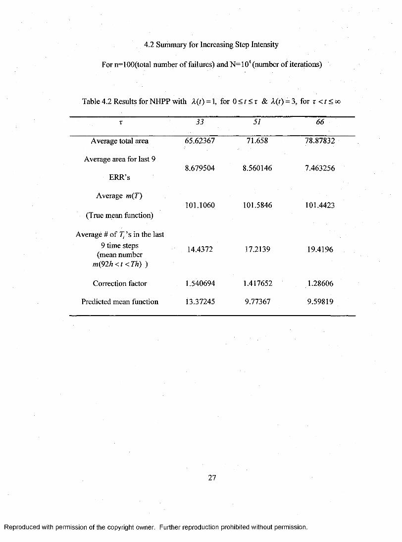
4.2 Summary for Increasing Step Intensity

For n=100(total number of failures) and N=10'‘ (number of iterations)

Table 4.2 Results for NHPP with X{t) = 1, for 0 < r < r & A(r) = 3, for T < r < oo

T 33 51 66



ERR’s8.679504 8.560146 7.463256

Average m{T)

(True mean function)101.1060 101.5846 101.4423

Average # of 7] ’s in the last9 time steps

(mean number m(92/;<r<7%) )

14.4372 17.2139 19.4196

Correction factor 1.540694 1.417652 1.28606

Predicted mean function 13.37245 9.77367 9.59819

27


4.3 Summary for Decreasing Step Intensity

For n=I 00(total number of failures) and N= 1 O'* (number of iterations)

Table 4.3 Results for NHPP with A(r) = 3, for 0 < r < t & X{t) = 1, for t < r < oo

T 52/9 669



ERR’s8.985952 9.027335 9.062618

Average m{t)

(True mean function)100.7025 100.5044 100.5679

Average # of 2] ’s in the last9 time steps

(mean number m(92h <t < Th) )

7.1816 6.2517 5.4808

Correction factor 0.717913 0.70243 0.729812

Predicted mean function 6.45113 6.34107 6.614007

28


4.4 Description of the Simulation Results

From the simulation, we get the total area under ERR curve and the true mean

funetion. The correction factor is also calculated based on the average values of the above

two, after lO" iterations. We can justify the correction factors from table 4.1 as follows.

The correction factor for = 0.5 is less when compared to = 1 & 2 because for p = 0.5,

the intensity function is decreasing, the number of events present initially will be more

when compared to that at the end. So there is an over estimate of number of events at the

end of given time period. In order to normalize it, the correction factor should be low so

when we get the actual number of events by multiplying the respective area with the

correction factor, we get a less number and there is no over estimation. And in case of

p = 2, since the intensity is increasing, initially there will be less events so there could be

under estimation of the number of events and hence the correction factor is high to

balance it. And for P =1, since there is no under or over estimation the correction factor

is almost equal to 1.

The averages o f the area for the last nine time-steps and the actual mean number

(i.e. the number of failures in the last nine time steps) are calculated. The average area for

last nine time-steps is multiplied with the correction factor in the simulation itself to gi ve

the predicted mean function. And from the results, it is evident that the predicted mean

function for the last nine time-steps is approximately equal to the actual mean number in

table 4.1 and in table 4.3 whereas there is slight variation in table 4.2 because the

intensity is increasing step, so whenr <t <<x>, the number of failures will be thrice than

the failures before the jump. So the actual mean number will be slightly more than the

29


predicted mean function whereas this effect is compensated in decreasing case by taking

T = 33/3,51/3,66/3 even before generating the NHPP.

So the results are quite satisfactory to state that this correction factor could be

used to predict the mean function, and the intensity of that fore-coming failures could be

estimated by using the formula A (t|0)= ^ and the goal of this thesis is achieved.

30


CHAPTER 5

APPLICATIONS

The control of industrial accidents generally requires, from time to time, new

safety equipment, safety regulations, improved machinery, etc.; hence, one may expect

that the number of accidents occurring would tend to decrease with time. Because of

serious injuries or, perhaps, deaths that may occur as a result of an industrial accidents, it

is usually important to know whether or not the safety action are resulting in a significant

decrease in the number of accidents. The nonhomogeneous Poisson process with Weibull

intensity function may possibly be useful in measuring this decrease (Crow, 1974). The

technique described in chapter 3 can be well applied to the mining data to predict the

number of failures in the coming years. So we will able to find the intensity of the

accidents using this prediction.

5.1 Mining Data

The data in Table 5.1 (Maguire et al, 1952, Table 1) represent days between

explosions in mines in Great Britain involving more than 10 men killed. The data cover

the period from December 6, 1875 to May 29, 1951. Using the inferences in chapter 2 it

can be easily determined that the data represents an NHPP with decreasing trend.

31


Table 5.1 Time Intervals in Days between Explosions in Mines, Involving 10 Men

Killed, from 6 December 1875 to 29 May 1951

378 59 54 498 217 15636 61 217 49 120 4715 1 113 131 275 12931 13 32 182 20 1630

215 189 23 255 66 2911 345 151 195 291 217137 20 361 224 4 74 81 312 566 369 1815 286 354 390 338 135772 114 58 72 33696 108 275 228 19124 188 78 271 32950 233 17 208 330120 28 1205 517 312203 22 644 1613 171176 61 467 54 14555 78 871 326 7593 99 48 1312 36459 326 123 348 37

315 275 457 745 19

5.2 ERR-Plotting of Mining Data

ERR-plots for the observation period, (0, T], are produced respectively for the

mining data (Table 5.1). In this application we use h = 365. Because the sample total of

the 109 successive mine accidents is 26,263, in order to equally divide the total period

into 72 years, we take additional 17 days as the final observation but we don’t consider

that an accident took place on 17*** day. In this the first 62 years are used to predict the

mean function of the next 10 years. So now the total number of days of observation

isT = 26280. The ERR-plot is displayed in Figure 5.1.

32


Fig. 5.1 ERR Plot of Mining Data for Time-Step h = 365

h=365

OLDCLU

OOo00ooo

oo'’oo

CDOoÔ

iCD

‘ OOoooC»CX)OCOOoOOooooC)Ooo

CMooCD

oooCD

10 20 30 400 50 60 70

Time-step

5.3 Predicting the Mean Function

The area under the ERR curve of mining data is calculated for 62 time-steps

(years) and the true mean function in the 62 years is found to be 98(i.e. the number of

accidents). The correction factor is determined hased on the above two which is given in

table 5.2. To get the maximum likelihood estimators of p and 9 over 62 years, we take

additional 13 days as the 99* observation, so, there are T = 22630 total days in the data

which is a multiple of 365. Now and Ô are determined to find the expected mean

function m{t^^^ = {T Iê ) , and it is found to be the same as the true mean number 98.

The results are given in table 5.2

33


Table 5.2 Results for the First 62 years

Total area for 62 time steps 135.7342

Correction factor 0.7219992

P 0.7221503

9 39.01416

^(^ 6 2) 98.9999

The actual mean number is determined for each year, after 62 years and their

cumulative numbers are also calculated. Now the area for each time-step under the ERR

curve is calculated along with the cumulative areas after 62 years which is multiplied

with the correction factor to predict the mean fimction in the last ten time steps.

The expected mean function is also determined for the last ten time steps using

. _ , . ' , f22630+365Â:Y , , _ _the Power Law process formula = 1,2,...,10 . The\ 9 J

cumulative mean function is calculated by the formulam(t(62<A<62+t)) = ^(^62+*) “ '” ( 6 2) •

And this when compared to the predicted mean function is proved from table 5.3

to be approximately equal. Although the actual mean numbers vary during the first few

years they are approximately equal to the predicted values in the final years. Hence, this

correction factor could be used to predict the mean function in the coming years, i.e., the

number of accidents in the coming years.

34


5.4 Summary of the Simulation Results for Mining Data:

Table 5.3 Results for the Last Ten years, with C.F = 0.7219992

No. o f No o f Cum No Cum area o f Cum m(t) CF * cum area

time steps failures in (actaul time steps Power Law o f each step

each step mean

number

m(t))

process (predicted

(■{62<h<62+k)) )

1 4 4 1.599846 1.150545 1.155088

2 1 5 3.214058 2.296026 2.320547

3 0 5 4.811053 3.436545 3.473576

4 0 5 6.383664 4.572199 4.609000

5 0 5 7.932623 5.703082 5.727348

6 2 7 9.473339 6.829285 6.839743

7 3 10 11.028006 7.950895 7.9262212

8 0 10 12.582044 9.067997 9.084225

9 0 10 14.114036 10.180674 10.190322

10 1 11 15.631543 11.289005 11.285961

35


CHAPTER 6

CONCLUSIONS AND FUTRUE WORK

6.1 Conclusions

The main goal of this thesis is to estimate the mean function of a monotonie point

process with a discrete time series. The relation between HPP and NHPP is well

established by proving the theorem, which is used to generate NHPP in the simulation.

The bridge between Poisson process and time series is easily demonstrated which can be

very helpful to get recurrence rates from any kind of Poisson process. The method to

predict the mean function of NHPP using area under ERR curves and the correction

factor proves to be useful as the correction factor given can be extended to the fore-

coming failures. The correction factor is well justified for three different recurrence rates.

The proposed algorithm to generate NHPP, to find the actual mean number, to get the

area under ERR curve and finally to calculate the correction factor after finding the true

mean function using the formula from Power law Process, shows tremendous potential to

forecast NHPP with various forms of intensity function and recurrence rates. Applying

the above technique to forecast the intensity of the accidents in the mining data is proved

to be successful from the results, even though there is slight variation in the predicted and

actual mean numbers for the first few time-steps, the mean function from the Power law

Process is approximately equal to the predicted one.

36


6.2 Future Work

From the results it is noticeable that the predicted mean function for increasing

step intensity differs from the actual mean number. The reason for that could be the

selection of jump points. So, this can be rectified in the future by properly analyzing the

jump points of the step, both for increasing and decreasing step intensity.

Finally for predicting the intensity of the NHPP, the predicted mean fonction

could be used and safety measures could be followed to avoid failures such as accidents

in the mining data.

37


CHAPTER?

R-PROGRAM

Given are the programs to find the total area, area for last 10 ERR’s under ERR

curve, number of time intervals in the last ten time sets, observed mean function and the

correction factor for the NHPP;

7.1 Program for p = 0.5,1,2

beta - 0.5 # modify to 1, 2for(r in 1:10000) {g = 0theta - 1X = rexp( 100,1)for(k in 1;100){z[k] = sum(x[l :k])t[k] = (th*((z[k])^(l/beta)))}betahat = 100/log(prod((t[100])/t[l :99]))thetahat = ((t[100])/( 100^(1/betahat)))h = (t[100])/100 #meanT-((t[100]/h)+l)for(jinl:T){w[j] = (j*h)for(i in 1:100) { if(t[i]<wD]){ g = g+l}} yD] = (g/w[j]) g = 0} d = 0for(i in 1:100) {if(t[i]<w[92D{d = d+l}}Numoft = (100-d)

38


soy = sum(y[92;101])areasmall[r] = ((soy-(y[92]/2)-(y [ 101 ]/2))*h) f = CLomsum(y)arealarge[r] = ((f[101]-(y[l]/2)-(y[101]/2))*h) expez[r] = ((T*h/tethahat)^(betahat)) truez[r] = ((T*h/theta)^beta)} totalareasmall = cumsiun(areasmall) avgarealastlOERR = totalareasmall [10000]/10000 totalnumoft = cumsum(numoft) avgnumoft = (totalnumoft[l 0000]/10000) totalarealarge - cumsum(arealarge) avgtotalarea = totalarealarge[ 10000]/10000 totalexpez = cumsum(expez) avgexpez = totalexpez[10000]/10000 totaltruez = cumsum(truez) avgtruez = totaltruez[ 10000]/l 0000correctionfactor = avgtruez * avgarealastlOERR / avgtotalarea

7.2 Program for Increasing Step Intensity

tau = 33 # modify to 51, 66 for(r in 1:10000){g = 0X - rexp( 100,1)for(kinl:100){z[k] == sum(x[l:k])if(z[k] < tau){t[k] = z[k]}if(z[k] > tau){t[k] = (z[k]+(2*tau))/3}}h = (t[ 100])/100 #meanT = ((t[100]/h)+l)for(jinl:T){wü] = (j*h)for(i in 1:100){ if(t[i]<wD]){ g = g+l}} y[j] = (g/w[j]) g = o} d = 0for(i in 1:100) { if(t[i]<w[92]){ d = d+l}}

39


Numoft = (100-d) soy - sum(y[92:101])areasmall[r] = ((soy-(y[92]/2)-(y[101]/2))*h) f=cumsum(y)arealarge[r] - ((f[101]-(y[l]/2)-(y[101]/2))*h)capt[r] = (T*h)traez[r] = (3*capt)-(2*tau)}totalareasmall = cumsum(areasmall)avgarealastlOERR = totalareasmall [10000]/10000totalnumoft = cumsum(numoft)avgnumoft = (totalnumoft[l 0000]/l 0000)totalarealarge = cumsum(arealarge)avgtotalarea - totalarealarge[l0000]/l0000totalcapt - cumsum(capt)avgcapt = totalcapt[10000]/10000totaltruez = cumsum(truez)avgtruez - totaltruez[ 10000]/l 0000correctionfactor - avgtruez * avgarealastlOERR / avgtotalarea

7.3 Program for Decreasing Step Intensity

tau - 33/3 # modify to 51/3, 66/3 fbr(r in 1:10000) {g = 0x = rexp( 100,1)for(k in 1:100) {z[k] = sum(x[l :k])l[k] = (z[k]/3)if(l[k] < tau){t[k] = l[k]}if(l[k] > tau){t[k] = (z[k]-(2*tau))}}h - (t[l 00])/l 00 #meanT = ((t[100]/h)+l)for(jinl:T){w[j] = (j*h)for(i in 1:100) {if(t[i]<w[j]){g = g+l}}yD] = (g/wDl)g = 0}d = 0for(i inl:100){

40


if(t[i]<w[92]){ d = d+l}}Numoft = (100-d) soy = sum(y[92:101])areasmall[r] = ((soy-(y[92]/2)-(y[101]/2))*h) f = cumsum(y)arealarge[r] = ((fI101]-(y[l]/2)-(y[101]/2))*h)capt[r] = (T*h)traez[r] = (capt)+(2*tau)}totalareasmall = cumsum(areasmall)avgarealastlOERR = totalareasmall [10000]/10000totalnumoft = cumsum(numoft)avgnumoft = (totalnumoft[ 10000]/10000)totalarealarge = cumsum(arealarge)avgtotalarea = totalarealarge[10000]/10000totalcapt = cumsum(capt)avgcapt = totalcapt [10000]/10000totaltruez = cumsum(truez)avgtruez = totaltruez[10000]/10000correctionfactor = avgtruez * avgarealastlOERR / avgtotalarea

7.4 Program for Mining Data

t =c(378,36,15,31,215,11,137,4,15,72,96,124,50,120,203,176,55,93,59,315,59,61,1,13,189,345,20,81,286,114,108,188,233,28,22,61,78,99,326,275,54,217,113,32,23,151,361,312,354.58.275.78.17.1205.644.467.871.48.123.457.498.49.131.182.255.195.224.566.390.72.228.271.208.517.1613.54.326.1312.348.745.217.120.275.20.66.291.4.369.338.336.19.329, 330,312,171,145,75,364,37,19,156,47,129,1630,29,217,7,18,1357,17)h = 365m = cumsum(t)z =c(378,36,15,31,215,ll,137,4,15,72,96,124,50,120,203,176,55,93,59,315,59,61,1,13,189,345.20.81.286.114.108.188.233.28.22.61.78.99.326.275.54.217.113.32.23.151.361.312.354,58,275,78,17,1205,644,467,871,48,123,457,498,49,131,182,255,195,224,566,390,72,228.271.208.517.1613.54.326.1312.348.745.217.120.275.20.66.291.4.369.338.336.19.329, 330,312,171,145,75,364,13)r = cumsum(z)betahat = 99/log(prod(r[99]/r[l:98]))thetahat = (r[99]/(99 Y 1 /betahat)))fbr(j in 1:72){wD] = (j*h)for(i in 1:110){if(m[i]<w[j]){

41


g = g+l}} y[j] = (g/wDJ) g = o }for(p in 1;10){ d = 0 for(qinif((w[61 +p]<m[q])&(m[q]<w[61 +( 1 +p)])) { d = d+l}} nnm[p] = dsoy[p] = sum(y[(61+p):(62+p)])area[p] = ((soy(p]-(y[61+p]/2>(y[62+p]/2))*h)mt[p] = ((22630+(365*p)ythetahat)^betahat}for(p in 2;10){cumnum[l] = num[l]cumnum[p] = num[p]+cumnum[p-l]cumarea[l] = area[l]cumarea[p] = area[p]+cumarea[p-l]}f= sum(y[l:62])tarea = ((f-y[l]/2-y[62]/2)*h)fm = cumsnm(y)ttarea = ((fm[72]-y[l]/2-y[72]/2)=^h)cf = 98/tareafor(p in 1:10){cfarea[p] = cf*cumarea[p]mtl[p] = mt[p]-((22630/tii)^bh)}


REFERENCES

1. Ascher H. (1983). Discussion on statistical Methods in Reliability, by J. F.

Lawless. Technometrics v25, p.305-335.

2. Bain L. J. and Engelhardt, M. (1980). Inferences on the Parameters and current

System Reliability for a Time Truncated Weibull Process. Technometrics y. 22,

No .4, p.305-335.

3. Bain L. J. and Engelhardt, M. (1991). Statistical Analysis o f Reliability and Life-

Testing Models - Theory and Methods. f2"^ ed.). New York: Marcel Dekker

4. Box G.E.P., and Jenkins G.M. (1976). Time Series Analysis Forecasting and

Control, Holden Day.

5. Brockwell P. J. and Dayis R. A. (2003). Introduction to Time Series and

Forecasting. Springer Texts in Statistics.

6 . Crow L. H. (1974). Reliability Analysis for Complex Repairable Systems.

reliability and biometry, eds. pp. 379-410.

7. Ho C.-H. (1993). Forward and Backward Tests for an Abrupt Change in the

Intensity of a Poisson Process: J. Statist. Comput. Simul. y.48, No.2, p. 245-252.

8 . Michael E. K., Halim D. and James R. W. (1998). Least squares estimation of

Nonhomogeneous Poisson process: Proceedings of 1998 Winter Simulation

Conference D.J. Medeiros, E.F. Watson, J.S. Carson and M.S. Maniyannan, eds.

43


9. NIST/SEMATECH e-Handbook of Statistical Methods,

http://www.itl.nist.gov/div898/handbook/,7/l 8/2006.

10. Reliability, Wikipedia contributors, 12/4/2006

http://en.wikit)edia.org/w/index.php?title=Reliabilitv&oldid=92020435

11. Rigdon S. E. and Basu A. P. (2000). Statistical Methods for the Reliability of

Repairable Systems

44


http://www.itl.nist.gov/div898/handbook/,7/l

http://en.wikit)edia.org/w/index.php?title=Reliabilitv&oldid=92020435

VITA

Graduate College University of Nevada, Las Vegas

Sandhya Gunti

Local Address:4217, Grove Circle, Apt#l,Las Vegas, Nevada, 89119

Degrees:Bachelor of Engineering, Electrical and Electronics Engineering, 2003 Univ. College of Engineering, Osmania University, Hyderabad, India.

Thesis Title:A Method for Estimating Intensity of a Poisson Process

Thesis Examination Committee:Chairperson, Dr. Chih-Hsiang Ho, Ph. D.Committee Member, Dr Malwane Ananda, Ph. D. Committee Member, Dr Hokwon Cho, Ph. D.Graduate Faculty Representative, Dr. Shizhi Qian, Ph. D.

45


a method for estimating intensity of a poisson process

Documents