a mesh optimization algorithm based on neural networks

Information Sciences 177 (2007) 5347–5364

www.elsevier.com/locate/ins

A mesh optimization algorithm based on neural networks q

Rafael Alvarez, Jose-Vicente Noguera, Leandro Tortosa *, Antonio Zamora

Departamento de Ciencia de la Computacion e Inteligencia Artificial, Universidad de Alicante, E-03080 Alicante, Spain

Received 22 February 2006; received in revised form 12 May 2007; accepted 16 May 2007

Abstract

We have developed a mesh simplification method called GNG3D which is able to produce high quality approximationsof polygonal models. This method consists of two distinct phases: an optimization phase and a reconstruction phase. Theoptimization phase is developed by applying an extension algorithm of the growing neural gas model, which constitutes anunsupervised incremental clustering algorithm. The primary goal of this phase is to obtain a simplified set of vertices rep-resenting the best approximation of the original 3D object. In the reconstruction phase we use the information provided bythe optimization algorithm to reconstruct the faces obtaining the optimized mesh as a result. We study the model theoret-ically, analyzing its main components, and experimentally, using for this purpose some 3D objects with different topolo-gies. To evaluate the quality of approximations produced by the method proposed in this paper, three existing errormeasurements are used. The ability of the model to establish the number of vertices of the final simplified mesh is dem-onstrated in the examples.� 2007 Elsevier Inc. All rights reserved.

Keywords: Neural networks; Growing neural gas; Mesh optimization; Surface reconstrucion; Mesh generation

1. Introduction

Current computer graphic tools allow design and visualization of more and more realistic and precise 3Dmodels. These models are numerical representations of both the real and imaginary worlds. Acquisition anddesign techniques of 3D models (modeler, scanner, sensor, etc.) usually produce huge data sets containing geo-metrical and appearance attributes. These devices generate meshes of great complexity to represent the models.

Simplification is mandatory when one has to manage the meshes produced by 3D scanning devices. Thesampling resolution of current scanning instruments produces surface meshes composed by 20–100 M faces.Meshes of this size usually have to be reduced to a more easily manageable size to be used in real applications.Therefore, the objective is clear: to produce a model that is visually similar to the original model and containsfewer polygons. Some techniques offer efficient processing but produce simplified meshes which are visuallyundesirable. Others create more pleasing approximations but are slow and difficult to implement.

0020-0255/$ - see front matter � 2007 Elsevier Inc. All rights reserved.

doi:10.1016/j.ins.2007.05.029

q This work was partially supported by the Spanish Grant GV06/018.* Corresponding author. Tel.: +34 965110083; fax: +34 965672426.

E-mail addresses: [email protected] (R. Alvarez), [email protected] (J.-V. Noguera), [email protected] (L. Tortosa), [email protected] (A. Zamora).

mailto:[email protected]



mailto:zamora@ dccia.ua.es

mailto:zamora@ dccia.ua.es

5348 R. Alvarez et al. / Information Sciences 177 (2007) 5347–5364

Over the last decades a tremendous amount of work has been done on mesh simplification. Most of thetechniques or algorithms proposed to accomplish this objective are based on reducing the mesh complexityeither by merging/collapsing elements or by re-sampling vertices. A good overview of the state of the art inthis field is [19]. Simplification strategies may be broadly grouped into two categories: local strategies that iter-atively simplify the mesh and global strategies that are applied to the input mesh as a whole.

Local strategies are the most common and some examples are the following ones:

• Vertex Decimation, first proposed by Schroeder et al. [23], operates on a single vertex by deleting that vertexand re-tesselating the resulting hole. The algorithm operates by making multiple passes over all the verticesof the model. A Bayesian technique for the reconstruction and subsequent decimation of 3D surface modelsfrom noisy sensor data can be seen in [6].

• Re-Tiling Polygonal Surfaces. The paper by Turk [24] describes a method to simplify arbitrary polyhedralobjects and works best on smoothly curved surfaces without shape edges or discontinuities.

• Edge Contraction, originally proposed by Hoppe et al. [15], is a common simplification operation. An edgecontraction operates on a single edge and contracts it to a single vertex, updating all edges previously inci-dent on it. Heckbert and Garland [12] showed that, under the L2 metric, this strategy produces optimal tri-angulations in the limit as the number of triangles goes to infinity and their area goes to zero. Garland andZhou [10] described a generalized version for high dimensions. See [1,26] for recent papers in this context.

Some representative examples of global simplification strategies are

• Shape Approximation, proposed by Coen-Steiner et al. [4]. They employ a variational partitioning schemeto segment the input mesh into a set of non-overlapping connected regions, and then fit a locally approx-imating plane to each one.

• Vertex Clustering, originally proposed by Rossignac and Borrel [22] to handle meshes of arbitrary topolog-ical structure.

In recent years, the problem of mesh simplification has received increasing attention. Several different algo-rithms have been formulated for simplifying meshes. Isenburg and Lindstrom [16] describe a streaming formatfor polygon meshes, which is simple enough to replace current mesh formats and more suitable for workingwith large data sets. Vieira et al. [25] propose the new stellar mesh simplification method based on a proba-bilistic optimization algorithm. A novel approach that express surface reconstruction as the solution to a Pois-son equation can be seen in [18]. Some other recent papers in this area are [2,5].

However, the algorithm we propose in this paper follows a different approach. It is based on artificial neuralnetworks, that were introduced as a concept in the 40s, but the first practical applications started to emerge inthe last two decades. A comprehensive introduction into the mathematical theory of neural networks can befound in [11]. During the last two decades, neural networks have found a lot of applications in such diverseareas, as pattern recognition, medical diagnosis, bio-informatics, hand-writing recognition and finance, tomention only few of them.

In this paper we use neural networks, in particular an adaptation of Fritzke’s Growing Neural Gas (GNG)algorithm [8] for mesh generation, with the aim of approaching the problem of surface optimization andreconstruction. The GNG algorithm has its origin in the Neural Gas algorithm [20] and the Growing CellStructure (GCS) algorithm [7]. These algorithms constitute perfect examples of growing or incremental net-work models, which are generated by successive addition (sometimes occasional deletion) of elements.

The GNG algorithm is also based on a graph but requires no determination of the network dimensionalitybeforehand as in GCS. Instead, the network starts with two units at random positions and inserts new nodesat positions with high errors. These nodes are connected by edges with a certain age. Old edges are removed,resulting in a topology preserving map with an induced Delaunay triangulation. After a fixed number of learn-ing steps multiplied with the actual number of nodes a new node is inserted between the location with the high-est error or signal counter and the highest one of all its neighbors.

We have developed an algorithm to simplify any three-dimensional mesh, with the primary characteristicssummarized in the following:

R. Alvarez et al. / Information Sciences 177 (2007) 5347–5364 5349

• It allows to establish the total number of vertices that will have the simplified object, that is, the level ofdetail that will have the resulting mesh.

• It allows to establish the running time to obtain the simplified mesh. This characteristic permits to use thealgorithm in real-time systems, where it becomes necessary to obtain a mesh simplification satisfying adeadline regardless of the level of detail.

2. An overview of the growing neural gas model

The GNG algorithm is an unsupervised incremental clustering algorithm. Given some input distribution inRn, it incrementally creates a graph, or network of nodes, where each node in the graph has a position in Rn.One of the primary characteristics of GNG is that it is an adaptive algorithm, in the sense that if the inputdistribution slowly changes over time, GNG is able to adapt, that is, to move the nodes so as to cover thenew distribution.

Starting with two nodes the algorithm constructs a graph in which nodes are considered neighbors if theyare connected by an edge. The neighbor information is maintained throughout execution by a variant of com-petitive Hebbian Learning, [21]. The variant can be summarized saying that for each input signal n, an edge isinserted between the two closest nodes, measured in Euclidean distance. GNG only uses parameters that areconstant in time. Insertion of new nodes ceases when a user-defined performance criteria is met or alternativelyif a maximum network size has been reached. In the following, we consider networks consisting of

• a set A ¼ fn1; n2; . . . ; nNg of nodes (it is equivalent to use the term vertices or neurons to refer to the nodesof the network),

• a set E ¼ fe1; e2; . . . ; eLg of connections or edges among node pairs.

2.1. The GNG algorithm

The GNG algorithm assumes that each node k consists of the following:

• wk, a reference vector, in Rn.• errork, a local accumulated error variable.• A set of edges defining the topological neighbors of node k.

The reference vector may be interpreted as the position of a node in input space. The local accumulatederror is a statistical measure that is used to determine appropriate insertion points for new nodes. Further-more, each edge has an age variable used to decide when to remove old edges in order to keep the topologyupdated. The GNG algorithm can be described as

INIT: Start with two nodes a and b at random positions wa and wb in Rn.

(1) Generate an input signal n according to P ðnÞ.(2) Find the nearest node s1 and the second nearest s2.(3) Increment the age of all edges emanating from s1.(4) Add the square distance between the input signal and the nearest node in input space to a local counter

variable:

Derrorðs1Þ ¼ kws1� nk2

:

(5) Move s1 and its direct topological neighbors towards n by fractions �b and �n, respectively, of the totaldistance:

Dws1¼ �bðn� ws1

Þ;Dwsn ¼ �nðn� wnÞ;

where n represents all direct neighbors of s1.
(6) If s1 and s2 are connected by an edge, set the age of this edge to zero. If such an edge does not exist, create it.


(7) Remove edges with an age larger than amax. If this results in points having no emanating edges, removethem as well.

(8) If the number of input signals generated so far is an integer multiple of a parameter k, insert a new nodeas follows:
• Determine the node q with the maximum accumulated error.• Insert a new node r halfway between q and its neighbor f with the largest error variable:
wr ¼ 0:5ðwq þ wf Þ:• Insert edges connecting the new node r with nodes q and f, and remove the original edge between q

and f.• Decrease the error variables of q and f by multiplying them with a constant a. Initialize the error var-

iable of r with the new value of the error variable of q.

(9) Decrease all error variables by multiplying them with a constant d.(10) If a stopping criterion is not yet fulfilled go to step 1.

The GNG network is able to make the important topological relations in a given distribution P ðnÞ of inputsignals explicit. A primary characteristic of this method is the incremental character of the model which elim-inates the need to specify a network size in advance. The growth process is carried on until a user-defined per-formance criterion on network size is met.

2.2. The drawbacks of GNG for mesh optimization

The GNG model presents some drawbacks itself when it is applied to the problem of mesh optimization forthree-dimensional objects in computer graphics.

The first problem we find is that GNG model only provides information about the nodes or vertices and theedges that connect them. There is no information about the triangles or faces of the mesh that makes thereconstruction of the object possible. Consequently, when GNG model is applied to the problem of 3D meshoptimization, a set of unorganized points and a set of edges connecting some of these points are obtained.Notice that a set of triangles (faces of the 3D object) are required to reconstruct the model.

In Fig. 1 we show an example of the GNG algorithm applied over a 3D object (a sphere). The snapshots inthe image show that the GNG model generates the position of a set of vertices for the optimized object and aset of edges but, what is more relevant for us, no face is obtained in the optimized mesh.

Fig. 1. Two snapshots of the GNG original algorithm trying to optimize a sphere.

Fig. 2. Execution example of the GNG algorithm over a simple part of an object. The top line represents the original object, while thebottom line represents the neural net.


The second problem of the GNG model is the existence of inactive nodes that produces the convergence ofthe algorithm towards a local minimum. These undesirable nodes generate foldovers in the new mesh. TheGNG algorithm provides a way to delete the inactive nodes employing the maximum age of an edge (amax).Nevertheless, this is not the most appropriate elimination method for our objective. As it will be shown in anexample, this strategy leads us to the problem of the existence of local minima that reduces the accuracy of thegenerated meshes.

The problems arising when some edges are eliminated using the amax variable, after several iterations of thealgorithm, are summarized in Fig. 2.

Let us suppose that Fig. 2a represents the state of the network at the ith iteration. Let us assume that thenodes marked as triangles are winners (labeled as s1 nodes), in two different iterations (we mean that they arenot consecutive iterations). As a consequence of the step 3 of the algorithm, all the edges emanating from themwill increase their age by one, as we can see in the Fig. 2b. Let us suppose that the second nearest nodes to thewinner ones (labeled as s2 nodes) are marked as a diamond. As described in step 6 of the algorithm, the exist-ing edge connecting both nodes (s1 and s2) will be reset to zero, see Fig. 2c.

This process will continue in forthcoming iterations of the algorithm. Notice that in each iteration the win-ner node can only be one of the nodes near the original (white circles, diamonds or triangles) and never will beone of the black circles. Besides, we have also assumed that the nodes marked as black circles are farther thanthe nodes marked as diamonds respect to the winner nodes (marked as triangles) and, as a consequence of this,their edge age will be increased and it will not be reset to zero.

When the network reaches the situation that Fig. 2d shows, the edges between triangle and black circlenodes are greater than the maximum edge age amax, therefore they will be removed, (see step 7 of the algo-rithm). However, the nodes marked as black circles in the figure will not be removed in this step because thereare edges connecting them to other nodes, as we see in Fig. 2e.

These black nodes will remain in the network and never will be referenced in the future. In Fig. 2f we showa possible overlapping of faces in the optimized mesh because the four disconnected nodes are also used toreconstruct the faces.

3. The growing neural gas 3D method

Section 2.2 summarized the drawbacks that the GNG method presents when we try to apply it to the prob-lem of mesh optimization in 3D models. However, it presents a very interesting property that may be very


useful for our objective. This characteristic is that the GNG method is able to find a distribution of the neu-rons that minimizes the distance between them and the input signals; in our case, the input signals are the ver-tices of the original mesh. So, we use this model as a basis to construct our method.

In broad terms, the growing neural gas 3D (GNG3D) method that we propose in this paper consists on twodifferent phases:

Phase 1: Mesh optimization.Phase 2: Mesh reconstruction.

Phase 1 consists on a modification of the GNG model introducing the possibility to remove some nodes orneurons that do not provide relevant information about the original model as we described in Section 2.2.After this phase we obtain a cloud of points and edges connecting them, but we have no information aboutthe faces of the simplified mesh. In Phase 2 we have developed a method to construct the faces of the optimizedmesh from the information provided by Phase 1. As this information permits us to reconstruct the simplifiedmesh, we name it the reconstruction phase. We describe in detail both phases in the following.

3.1. Phase 1. Mesh optimization

The primary objective of this optimization phase is the calculation of the best vertices distribution thatshapes the new simplified mesh. The core of this phase is the implementation of an optimization algorithmsimilar to the GNG algorithm described in Section 2. The details of this algorithm are described in thefollowing:

Optimization algorithm

INIT: Start with two nodes a and b at random positions wa and wb in Rn. Initialize the error variable to zero.

(1) Generate an input signal n according to P ðnÞ.(2) Find the nearest node s1 and the second nearest s2 to the input signal.(3) Increment the age of all edges emanating from s1. If the age of any edge is greater than amax, then mark it

in order to be eliminated afterwards.(4) Increment the local activation counter variable of the winner node. Add the square distance between the

input signal and the nearest node in input space to a local error variable:

Derrorðs1Þ ¼ kws1� nk2

:

Store the nodes with the highest and lowest value of the local counter variable
(5) Move s1 and its direct topological neighbors towards n by fractions �b and �n, respectively, of the total
distance:

Dws1¼ �bðn� ws1

Þ;Dwsn ¼ �nðn� wnÞ;where n represents all direct neighbors of s1.

(6) If s1 and s2 are connected by an edge, set the age of this edge to zero. If such an edge does not exist, create it.(7) Remove edges with an age larger than amax. If this results in nodes having no emanating edges, remove

them as well.(8) Decrease the error variables of all the nodes by multiplying with a constant d.(9) Repeat steps 1 to 8 k times, with k an integer.

• If the maximum number of nodes has not been reached then insert a new node as follows:– Determine the node q with the maximum accumulated error.– Insert a new node r halfway between q and its neighbor f with the largest error variable:

wr ¼ 0:5ðwq þ wf Þ:
– Insert edges connecting the new node r with nodes q and f, and remove the original edge between q
and f.


– Decrease the error variables of q and f by multiplying them with a constant a. Initialize the errorvariable and the local counter of node r with the new value of the error variable and local counterof q, respectively.

• If the maximum number of nodes has been reached then remove a node as follows:– Let k be the stored node with the lowest error variable.– Remove node k and all the edges emanating from k.

(10) If N is the total number of nodes, every l � N iterations of steps 1 to 8 remove all the nodes that have notbeen used (local activation counter equal to zero) and all the edges emanating from them. Reset the localcounter of all the nodes to zero.

Some basic characteristics of this algorithm must be remarked

• The accumulated error of nodes in step 4 is a quantity that allows us to determine the regions wherethere is a low density of nodes according to the vertices existing in the original 3D object. Regionswhere the accumulated error is high are suitable candidates for being covered with new nodes orneurons.

• The local activation counter variable is useful to eliminate nodes and avoid the problem of local minima.• Parameters �b; �n; d; k; a, and l are not fixed. They are obtained experimentally.• The parameter k is just used to determine the moment to insert a new node in the mesh.• The parameter l is used to determine when to eliminate a node that has not been referenced in the previous

iterations.

Although the optimization algorithm is somewhat similar to the GNG algorithm, it presents a veryimportant difference. In our algorithm the nodes and the edges emanating from them that have not beenreferenced along the process of constructing the optimum neural network, are removed. This is carriedout by the introduction of a local counter variable in the step 4 of the algorithm. This local activationcounter gives us the information about the number of times that a node has been referenced as thewinner in the process of determining the closest node to the input signal. The introduction of thiscounter for each node is related with the ‘‘removing task’’ in the step 10 of the algorithm, where the nodesthat have never been referenced as winners are removed. The edges emanating from these nodes are alsoremoved.

In this way, we avoid the generation of foldovers that appear in practice when we carry out the face recon-struction of the simplified model. This can be solved because the nodes that generate this problem have a com-mon characteristic: they have not being referenced; consequently, they will be removed when the step 10 is run.Then, these nodes do not appear in the final simplified mesh.

3.2. Phase 2. Reconstruction of the 3D object

As a consequence of the fact that GNG model provides no information about the triangles or faces of thesimplified mesh, we need to develop a second phase to complete a suitable reconstruction of the 3D object; thisconstitutes one of the main contributions of the model proposed in this paper.

In general, phase 1 can be seen as a training process based on neural networks. At the end of this process aset of nodes, representing the new vertices of the optimized mesh, is computed. The edges connecting thesenodes show the neighboring relations among the nodes generated by the optimization algorithm. This phasecan be run as many times as we want with the aim of obtaining the best node configuration in the new mesh.Once this process has been completed, we begin the second phase of reconstruction that is analyzed in thefollowing.

The reconstruction phase constitutes a post-process which uses the information about new nodes providedby the optimization phase and the information about the nodes of the original model. With these sets of nodes,a concordance process can be carried out between the nodes of the original object and the nodes generated bythe optimization algorithm. This concordance process allows us to reconstruct the faces of the newly opti-mized mesh. This reconstruction phase can be summarized in three steps:


(1) Associate a representative (node) to every node in the original mesh, making groups of nodes with thesame representative.

(2) Create a string with all the connections among the resulting groups.(3) Reconstruct the faces.

Step 1. Associate a representative (node) to every node in the original mesh, making groups of nodes with the

same representative

In this step, we must find the optimization set node that is closer to each node of the original mesh. Supposethat K ¼ fk1; k2; . . . ; kMg is the set of nodes (vertices) of the original object and A ¼ fn1; n2; . . . ; nNg is the set ofnodes obtained by the optimization algorithm. Then, for each ki 2 K we must find the representative of ki, thatis, the node nj 2 A which is closer to ki. This task must be repeated for every node of the original object.

As the number of vertices, or nodes, in the original object is generally very high, we use an octree with theaim of dividing the three-dimensional space in a balanced way and set bounds to the searching space in orderto speed up this step. An octree is a data structure to represent objects in the three-dimensional space, auto-matically grouping them hierarchically and avoiding the representation of empty portions of the space. Thefirst octree node is the root cell, which is an array of eight contiguous elements. In our case, we have imple-mented an octree of one level, where each son keeps an array of vertices or nodes that are placed in its region.

The problem that can arise when working with an octree structure is that dividing the space into regionsand searching only inside the region in which the original node is situated can give rise to an undesirable sit-uation. That is, we can chance upon the possibility that the representative node obtained in this step is not theoptimum. If it is not the optimum, at least it will be close to it. The worst case occurs when all the nodes mustbe checked to find the optimum; in this situation no benefit will be gained when using such structure. In theexperiments performed with different models and different topologies, these cases only arise in the early iter-ations of the algorithm, when the number of nodes is small.

We see an example of the reconstruction process in Fig. 3. For this example, a small mesh with 13 nodesand 25 edges is used and the steps leading to the reconstruction of the finally optimized model have been illus-trated. In Fig. 3a we have overlapped the original nodes of the model with the five nodes obtained after apply-ing the optimization algorithm. They have been labelled as 1,2,3,4,5. In Fig. 3b we have created the groups inthe original mesh according to their representative. Observe the drawn circles to point out the nodes havingthe same representative in the optimized mesh.

Step 2. Create a string with all the connections among the resulting groups

According to the operations of labelling carried out in the step 1, the nodes of the original mesh have beenarranged in groups and each one of these groups has associated one, and only one, node belonging to the

Fig. 3. Four images summarizing the steps leading to the reconstruction phase, applied over a small mesh.

Fig. 4. Reconstruction of a face following the steps described in this section.


group of nodes obtained after applying the optimization algorithm. Recall that the number of nodes in thesimplified mesh is much smaller than the number of nodes of the original object. This association of nodesis performed minimizing the distance among the two sets of nodes (the original set of nodes and the set pro-vided by the optimization algorithm). In this second step we continue analyzing each of the faces of the ori-ginal mesh to check if their vertices have a different representative. In other words, we are looking for trianglesin the original mesh where the representative nodes of the vertices belong to different groups. When a trianglewith this property is found, then it is necessary to store the connection among these groups for a further rep-resentation of these connections in the optimized mesh.

Continuing with the previous example, Fig. 3c shows the triangles with the characteristic exposed in thisstep. They have been labelled as a; b; c; d. The connections among these vertices are stored with the purposeof carrying out the reconstruction process.

Step 3. Reconstruct the faces

In this third step we proceed to obtain the faces of the optimized mesh. For this purpose, the key point is toscan the list of the representatives and when we find a connection among three neighboring groups, we con-clude that this face must be represented. We follow the illustration of this step by using the same example asbefore. Observe in Fig. 3c that there are four triangles verifying this characteristic, that is, the three vertices ofeach of the triangles have representatives in different groups. Therefore, it is necessary to trace the edges cor-responding to these representatives. As a consequence of this process, the faces are created and it is generatedthe simplified mesh shown in Fig. 3d, consisting of five nodes and eight edges.

Fig. 4 shows us a real 3D object (a human face) and the final reconstruction of faces after executing thethree steps which are the basis of this reconstruction phase. On the left picture, the groups of nodes of theoriginal mesh that have the same representative are shown in different tonalities. On the right picture, the sim-plifications that are carried out in each area of the original mesh are obvious, according to the steps describedabove. Note that the simplified mesh is much less complex than the original one; even obtaining this level ofsimplification, it is remarkable that it maintains the topology of the original object notably.

An algorithm for the optimization of 3D meshes based on GCS is described in [17] and it produces the faceinformation of the simplified object directly eliminating the need for a second phase. This method starts from aclosed tetrahedron and progressively adds faces until it reaches the desired resolution. This system has thedrawback that, since it is based on a closed object, it cannot be applied to simplify open objects. Another con-sideration is that the way of adding new faces is very restrictive in order to prevent face overlapping and tokeep the object closed. This restriction in the way of creating new faces makes it slower than the method pre-sented here that only considers vertex information.

4. Examples and results

In this section, we will report some experimental results to demonstrate the general behavior and perfor-mance of our model. This model has been implemented in C++ and it has been structured in a multithreaded


application. One thread executes the steps of the algorithm in a loop controlled by the control panel. This con-trol panel is a window dialog controlled by another thread which sends orders to the algorithm loop and con-trols the behavior of the third thread, the visualization window.

The control panel permits to send, in real time, to the algorithm loop all the possible configurable behav-iors. For example to pause and continue the loop, end the optimization phase and start the reconstructionphase, set the new values of the parameters, set the percentage of vertices for the optimized object basedon the original one, etc.

The visualization window shows in 3D the current state of the network at each iteration step of the algo-rithm and the original 3D object. It has been implemented in two versions: the first one allows to take advan-tadge of the new 3D acceleration graphic cards using the OpenGL library. The second one constructsmanually the image using the DirectX library. Each solution has both advantages and disadvantages. TheOpenGL solution uses the graphic processor and consumes less system processor time, but it requires an accel-erator graphic card and no control is taken in the pixel to pixel rendering. The DirectX solution permits tocontrol each rendered pixel in the screen and no accelerator graphic card is required, but it uses all the pro-cessor time to perform the calculations.

The control panel thread also permits to change the behavior of the visualization window, it allows tochoose the rendering method between wireframe, flat or gouraud shading. The rotation and translation ofthe 3D objects has been also implemented to improve the visualization and comparison of the two meshes.

The algorithm thread executes the steps of the optimization phase in a loop; when the control panel sendsthe order the reconstruction phase starts in order to get the faces of the reconstructed mesh. To handle all theelements needed in the neural network and to add or remove nodes and edges easily, it has been implementedas an indexed ordered list of nodes and an indexed ordered list of edges. With the objective to speed up thereconstruction face, an octree structure is used with the purpose of dividing the 3D space in a balanced way asdescribed in Section 3.2.

However, before showing the visualization of some 3D objects, we need to define a strategy to quantify thequality of the approximations that can be generated using the GNG3D method.

4.1. Evaluating approximations

An error measurement is required to evaluate the quality of approximations produced by our algorithm.This measurement let us determine how accurate our model is and if our training process is on the right track.

As explained in [13], the error of the approximation is typically measured with respect to L2 or L1 error.

The L2 error between two n-vectors u and v is defined as ku� vk2 ¼Pn

i¼1ðui � viÞ2h i1=2

. The L1 error, also

called the maximum error, is defined as ku� vk1 ¼ maxni¼1jui � vij. Optimization with respect to the L2

and L1 metrics are called least squares and minimax optimization, and such solutions are called L2-optimal

and L1-optimal, respectively. Distances can be measured in different ways, e.g., to the closest point on agiven polygon, or the closest point on the whole surface. Other error measurements can be found in[3,14].

We have used two methods of error evaluation. For the first one, we chose a metric which measures thesquared distance between the approximation and the original model as described in [9]. We define the distancedðv;AÞ ¼ minp2Akv� pk as the minimum distance from v to the closest vertex p in the optimized mesh. Thismetric provides two error measurements which allow us to evaluate the approximations we are generating.These error measurements are

• Mean error value of the minimum squared distance, given by

Eavg ¼1

jM jXv2K

d2ðv;AÞ:

• Maximum error value of the minimum squared distance, given by

Emax ¼ maxv2Kfd2ðv;AÞg:


Remember that K is the set of vertices of the original model, jM j is the number of elements of K, and A isthe set of vertices of the simplified object.

The second error measurement method computes the difference between the area comprised by the faces ofthe original object and the area corresponding to the faces of the simplified object [3]. Taking that the faces ofthe three-dimensional models considered here are triangular, this metric can be computed in the followingway:

Esur ¼ SK � SA

with

SX ¼1

2

Xf2X

va � vb � sena ¼ 1

2

Xf2X

j~va �~vbj

with X being the set of faces of the original mesh and va, vb the vectors joining the vertices belonging to face f.The quality of the generated mesh can be known at any time employing the metric of the distance to the ver-

tices on any iteration during the training of the neural network in phase 1. The area difference metric can only becomputed after applying phase 2 because there are no faces in the mesh being optimized during phase 1.

4.2. The parameters choice

To carry out our experiments we need first to specify a set of parameters for the optimization algorithm.The parameters involved in the algorithm are the following:

• amax, the maximum age for the edges,• �b, related to the displacement of the winner node in the space,• �n, related to the displacement of the neighbour nodes in the space,• d, a constant to decrease the error variables,• k, an integer to determine when to create a new node,• a, a constant to decrease the error variables of the nodes after adding a new one,• l, a constant to know when to remove the nodes that have not been referenced in successive iterations.

200

250

300

350

400

450

500

550

600

0 0.2 0.4 0.6 0.8 1

Eavg

Eb

Eavg

Fig. 5. Bull 3D model. The average error for the parameter �b.


There is no parameter set that can always produce the best results (lowest error values) for all possiblethree-dimensional models. The parameter values that minimize error for a certain model can achieve slightlyhigher error values for other models. This characteristic is common in all training processes based on neural

290

295

300

305

310

315

320

0 20 40 60 80 100

Eavg

Lambda

Eavg

Fig. 6. Bull 3D model. The average error for the parameter k.

250

300

350

400

450

500

550

600

0 0.01 0.02 0.03 0.04 0.05 0.06 0.07 0.08 0.09 0.1 0.11

Eavg

En

Eavg

Fig. 7. Bull 3D model. The average error for the parameter �n.


networks. Nevertheless, the simplified models present a very high similarity with the original object regardlessof parameter values, since the error is still very small.

As an example, we have taken the 3D model called Bull to perform an experimental analysis of the way thatthe value of the parameters influence the error achieved. We have fixed the values of all the parameters exceptthe one being studied. In this example, we have tested the Eavg obtained with the GNG3D method when the

0.06

0.07

0.08

0.09

0.1

0.11

0.12

0.13

0.14

0.15

0.16

0 0.2 0.4 0.6 0.8 1

Eavg

Eb

Eavg

Fig. 8. Octopus 3D model. The average error for the parameter �b.

0.065

0.07

0.075

0.08

0.085

0.09

0.095

0.1

0 20 40 60 80 100

Eavg

Lambda

Eavg

Fig. 9. Octopus 3D model. The average error for the parameter k.


parameter �b varies from 1 to 0.1, the parameter k varies from 5 to 100, and the parameter �n varies from0.00001 to 0.10000 for this model.

In Fig. 5 we show the error evolution (in this case Eavg), changing the parameter �b. Observing the resultsachieved, we can conclude that the lowest error is obtained when �b varies from 0.3 to 0.4. In Fig. 6 we showthe error evolution by changing the parameter k; in this case, the lowest error is obtained when k is equal to 85.

0.07

0.08

0.09

0.1

0.11

0.12

0.13

0.14

0.15

0 0.01 0.02 0.03 0.04 0.05 0.06 0.07 0.08 0.09 0.1 0.11

Eavg

En

Eavg

Fig. 10. Octopus 3D model. The average error for the parameter �n.

Fig. 11. Dragonfly (top), Gargoyle (middle), and Fetus (bottom) models reconstructed using the GNG3D method.


In Fig. 7 the study has been done for the parameter �n. We conclude that the value of this parameter should besmaller than 0.04 to produce good results. A similar study can be performed for the rest of the parameters.

As we have already remarked, these experimental results are only valid for this model. The results maychange for any other, as we can see in Figs. 8–10, where the model we have taken in this case is called Octopus.In this new example, we have tested, as in the previous one, the Eavg obtained with the GNG3D method whenthe parameter �b varies from 1 to 0.1, the parameter k varies from 5 to 100, and the parameter �n varies from0.00001 to 0.10000.

Observe that the best results of the Eavg for the parameter �b are exactly at 0.4 (see Fig. 8). The differencesrespect to Figs. 6 and 7 for the parameters k and �n are also remarkable.

4.3. Some examples

The GNG3D method described in the previous sections was tested using more than fifty 3D models. Ouralgorithm can produce high fidelity approximations of any 3D model. With the purpose of showing some

Table 1Iterations, vertices and faces for the examples shown in Fig. 11

Model Number of iterations Vertices Faces

Dragonfly (a) 10000 2k (3.99%) 5.8k (5.82%)Dragonfly (b) 50000 10k (19.93%) 24k (24.07%)Dragonfly (c) 200000 25k (50.00%) 47k (47.16%)

Gargoyle (a) 10000 1k (4.68%) 2k (5.33%)Gargoyle (b) 40000 4k (18.71%) 8k (19.95%)Gargoyle (c) 80000 8k (37.41%) 14k (35.50%)

Fetus (a) 5000 0.5k (4.01%) 1k (4.21%)Fetus (b) 25000 2.5k (19.97%) 4.5k (18.10%)Fetus (c) 50000 5k (39.93%) 8k (33.24%)Fetus (d) 100000 6k (50.00%) 10k (41.30%)

0

5

10

15

20

0 100000 200000 300000 400000 500000 600000 700000 800000

Err

or

Iterations

EavgEmax

Fig. 12. Graph showing the error decreasing during the optimization phase of the Fetus 3D model.

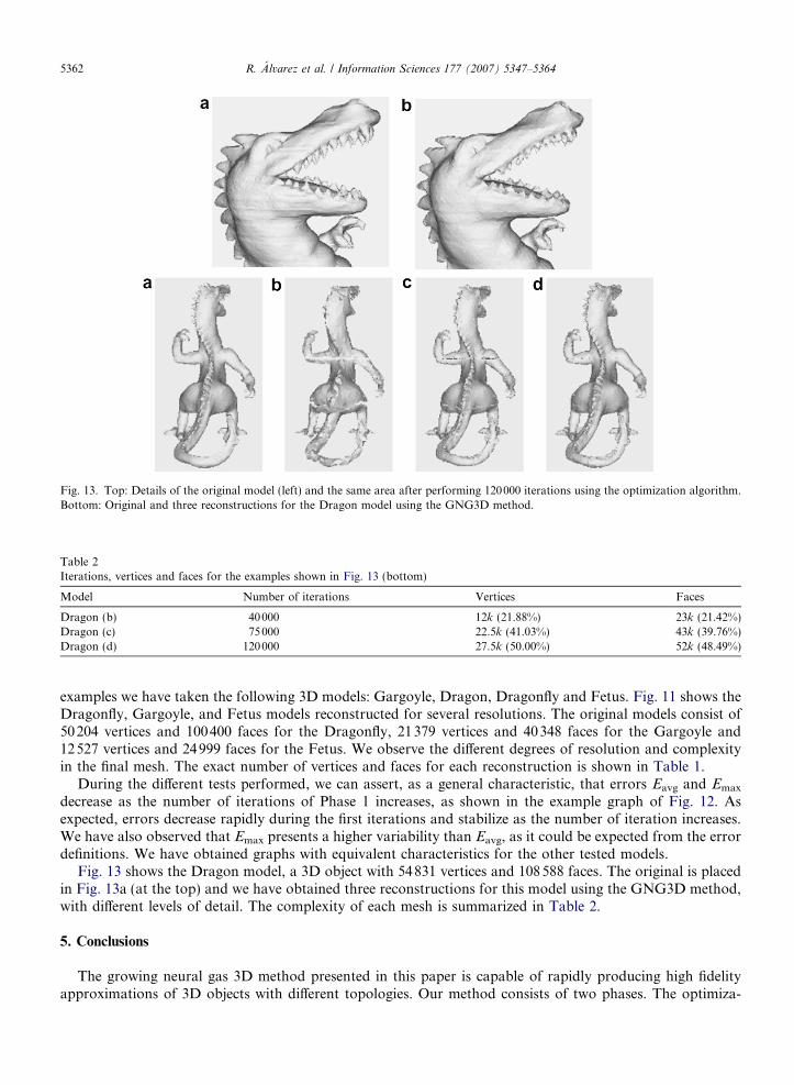
Table 2Iterations, vertices and faces for the examples shown in Fig. 13 (bottom)

Model Number of iterations Vertices Faces

Dragon (b) 40000 12k (21.88%) 23k (21.42%)Dragon (c) 75000 22.5k (41.03%) 43k (39.76%)Dragon (d) 120000 27.5k (50.00%) 52k (48.49%)

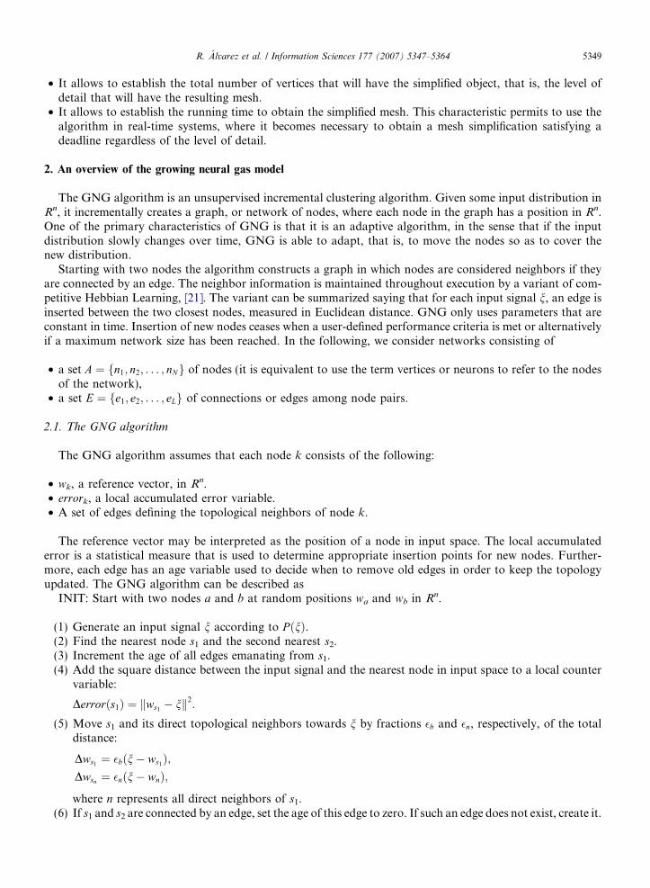
Fig. 13. Top: Details of the original model (left) and the same area after performing 120000 iterations using the optimization algorithm.Bottom: Original and three reconstructions for the Dragon model using the GNG3D method.


examples we have taken the following 3D models: Gargoyle, Dragon, Dragonfly and Fetus. Fig. 11 shows theDragonfly, Gargoyle, and Fetus models reconstructed for several resolutions. The original models consist of50204 vertices and 100400 faces for the Dragonfly, 21379 vertices and 40348 faces for the Gargoyle and12527 vertices and 24999 faces for the Fetus. We observe the different degrees of resolution and complexityin the final mesh. The exact number of vertices and faces for each reconstruction is shown in Table 1.

During the different tests performed, we can assert, as a general characteristic, that errors Eavg and Emax

decrease as the number of iterations of Phase 1 increases, as shown in the example graph of Fig. 12. Asexpected, errors decrease rapidly during the first iterations and stabilize as the number of iteration increases.We have also observed that Emax presents a higher variability than Eavg, as it could be expected from the errordefinitions. We have obtained graphs with equivalent characteristics for the other tested models.

Fig. 13 shows the Dragon model, a 3D object with 54831 vertices and 108588 faces. The original is placedin Fig. 13a (at the top) and we have obtained three reconstructions for this model using the GNG3D method,with different levels of detail. The complexity of each mesh is summarized in Table 2.

5. Conclusions

The growing neural gas 3D method presented in this paper is capable of rapidly producing high fidelityapproximations of 3D objects with different topologies. Our method consists of two phases. The optimiza-


tion phase represents an improvement respect to the algorithms using the GNG model, since we carry outthe suitable modifications in order to eliminate the undesirable vertices in the simplified mesh. However, themain contribution of our method is given by the reconstruction phase, which allows to reconstruct the 3Dobject in a quickly and efficiently way, using the set of vertices and edges provided by the optimizationphase.

Another excellent characteristic of the method proposed is that the training process in the optimizationphase can be continued until a user-defined criterion is reached.

In order to evaluate the quality of the approximations produced by the GNG3D method different existingerror measurements are used. This error metric also permits us to study the best values for the parametersinvolved in the optimization algorithm; understanding the best values as those which minimize the errorbetween the original and the simplified model.

The experimental results show that the simplified objects are generated very fast and with a high level ofapproximation respect to the original ones. Besides, for all the 3D models studied, the error measurementsdecrease as the number of iterations increases.

References

[1] M. Anderson, J. Gudmundsson, C. Levcopoulos, Restricted mesh simplification using edge contractions, 22nd European Worhshopon Computational Geometry, 2006, pp. 121–124.

[2] S. Atlan, M. Garland, Interactive multiresolution editing and display of large terrains, Computer Graphics Forum 25 (2) (2006) 211–224.

[3] P. Cignoni, C. Rocchini, R. Scopigno, Metro: measuring error on simplified surfaces, Computer Graphics Forum 17 (2) (1998) 167–174.

[4] D. Coen-Steiner, P. Alliez, M. Desbrun, Variational shape approximation, ACM Transactions on Graphics 23 (3) (2004) 905–914.

[5] L.-F. Diachin, P. Knupp, T. Munson, S. Shontz, A comparison of two optimization methods for mesh quality improvement,Engineering with Computers 22 (2) (2006) 61–74.

[6] J.-R. Diebel, S. Thrun, M. Brunig, A Bayesian method for probable surface reconstruction and decimation, ACM Transactions onGraphics 25 (1) (2006) 39–59.

[7] B. Fritzke, Growing cell structures – a self-organizing network for unsupervised and supervised learning, Neural Networks 7 (9)(1994) 1441–1460.

[8] B. Fritzke, A growing neural gas network learns topology, in: G. Tesauro, D.S. Touretzky, T.K. Leen (Eds.), Advances in NeuralInformation Processing Systems 7, MIT Press, Cambridge MA, 1995, pp. 625–632.

[9] M. Garland, P.S. Heckbert, Surface simplification using quadric error metrics, in: Proc. SIGGRAPH 97: Surface Simplification, 1997,pp. 209–216.

[10] M. Garland, Y. Zhou, Quadric-based simplification in any dimension, ACM Transactions on Graphics 24 (2) (2005) 825–838.[11] S. Haykin, Neural networks: a comprehensive foundation, Prentice Hall, NJ, 1998.[12] P. Heckbert, M. Garland, Optimal triangulation and quadric-based surface simplification, Journal of Computational Geometry:

Theory and Applications 14 (1–3) (1999) 49–65.[13] P.S. Heckbert, M. Garland, Survey of polygonal surface simplification algorithms, SIGGRAPH 97: draft course notes, 1997.[14] H. Hoppe, New quadric metric for simplifying meshes with appearance attributes, in: Proc. IEEE Visualization ’99, 1999, pp. 59-66.[15] H. Hoppe, T. DeRose, T. Duchamp, J. McDonald, W. Stuetzle, Mesh optimization, Computer Graphics 27, Annual Conference

Series, 1993, pp. 19–26.[16] M. Isenburg, P. Lindstrom, Streaming meshes, in: Proc. on Visualization’05, 2005, pp. 231–238.[17] I.P. Ivrissimtzis, W.-K. Jeong, H.P. Seidel, Using growing cell structures for surface reconstruction, in: Proc. International

Conference on Shape Modeling and Applications, 2003, pp. 78–88.[18] M. Kazdan, M. Bolitho, H. Hoppe, Poisson surface reconstruction, in: Eurographics Symposium on Geometry Processing, Cagliari,

Italy, 2006, pp. 26–28.[19] D.P. Luebke, A developer’s survey of polygonal simplification algorithms, IEEE Computer Graphics and Applications 21 (3) (2001)

24–35.[20] T. Martinetz, K.J. Schulten, A neural-gas network learns topologies, in: T. Kohonen, K. M Okisara, O. Simula (Eds.), Artificial

Neural Networks, Amsterdam, 1991, pp. 397–402.[21] T. Martinetz, Competitive Hebbian learning rule forms perfectly topology preserving learning, in: Proc. ICANN’93: International

Conference on Artificial Neural Networks, Springer-Verlag, Amsterdam, The Netherlands, 1993, pp. 427–434.[22] J. Rossignac, P. Borrel, Multi-resolution 3D approximation for rendering complex scenes, in: B. Falcidieno, T. Kunii (Eds.),

Geometric Modeling in Computer Graphics, Springer-Verlag, Genova, Italy, 1993, pp. 455–465.[23] W.J. Schroeder, J.A. Zarge, W.E. Lorensen, Decimation of triangle meshes, in: Proc. SIGGRAPH’92: 19th International Conference

on Computer Graphics and Interactive Techniques, Chicago IL, 1992, pp. 65–70.


[24] G. Turk, Re-Tiling polygonal surfaces, in: Proc. SIGGRAPH’92: 19th International Conference on Computer Graphics andInteractive Techniques, Chicago IL, 1992, pp. 55–64.

[25] A.W. Vieira, T. Lewiner, L. Velho, H. Lopes, G. Tavares, Stellar mesh simplification using probabilistic optimization, ComputerGraphics Forum 23 (2004) 825–838.

[26] J. Yan, P. Shi, D. Zhang, Mesh simplification with hierarchical shape analysis and iterative edge contraction, IEEE Transactions onVisualization and Computer Graphics 10 (2) (2004) 142–151.

a mesh optimization algorithm based on neural networks

Documents