A Memetic Approach toVehicle Routing Problem with Dynamic Requests

Jacek Mandziuka,b,∗, Adam Zychowskia

aFaculty of Mathematics and Information Science, Warsaw University of Technology,Koszykowa 75, 00-662 Warsaw, Poland

bSchool of Computer Engineering, Nanyang Technological University,Block N4, Nanyang Avenue, Singapore 639798

Abstract

The paper presents an effective algorithm for solving Vehicle Routing Problem

with Dynamic Requests based on memetic algorithms. The proposed method

is applied to a widely-used set of 21 benchmark problems yielding 14 new best-

know results when using the same numbers of fitness function evaluations as the

comparative methods. Apart from encouraging numerical outcomes, the main

contribution of the paper is investigation into the importance of the so-called

starting delay parameter, whose appropriate selection has a crucial impact on

the quality of results. Another key factor in accomplishing high quality results

is attributed to the proposed effective mechanism of knowledge transfer between

partial solutions developed in consecutive time slices. While particular problem

encoding and memetic local optimization scheme were already presented in the

literature, the novelty of this work lies in their innovative combination into one

synergetic system as well as their application to a different problem than in the

original works.

Keywords: vehicle routing, memetic algorithm, optimization under

uncertainty, scheduling, dynamic optimization

∗Corresponding authorEmail address: mandziuk@mini.pw.edu.pl (Jacek Mandziuk)

Preprint submitted to Applied Soft Computing January 12, 2016

1. Introduction

Vehicle Routing Problem (VRP), first introduced by Dantzig and Ramser

in [1], is an NP-hard combinatorial optimization problem with many practical

applications. In its classical formulation a set of customers must be served by a

fleet of homogenous vehicles (with some pre-defined capacity) with routes begin-5

ning and ending at a specified depot. The optimization goal is to minimize the

total routes’ length/cost of all vehicles. Due to the VRP’s combinatorial com-

plexity the exact solution methods proved inefficient, except for simple problems.

Therefore most of the research effort was devoted to application of metaheuris-

tic algorithms, for instance Ant Colony Optimization (ACO) [2], Tabu Search10

(TS) [3], Genetic Algorithms (GA) [4], Simulated Annealing (SA) [5] or Upper

Confidence Bounds Applied to Trees (UCT) [6], with promising results.

In majority of practical applications, however, another dimension related

to stochastic nature of the real-life problems is added to the problem’s formu-

lation. In particular, the information available at the beginning may change15

during the solution execution, for instance due to the arrival of new customers’

orders [7, 8] or because of the changes in their requested demands [9] or be-

cause of unplanned events, e.g. traffic jams/road congestion [10, 11] or, more

generally, due to stochastic travel times [12]. This intrinsic stochasticity of the

practical VRP realizations led to the extension of the static VRP to a class of20

Dynamic Vehicle Routing Problems (DVRP), solving which requires adequate

on-line routes’ adjustment in response to the arrival of new problem-related

information.

Furthermore, in the literature there are many variants of the VRP which are

formulated so as to serve specific practical needs, e.g. its multi-trip [13] or multi-25

compartment [14] versions, variants with specific time-windows for delivery[15],

formulations which combine delivery with picking up goods from the clients [16],

and many others (see the recent special issue [17] for an overview of the current

developments and challenges in this domain and [18] for the VRP taxonomy).

This paper considers a version of DVRP in which some of the customers’30

2

locations (and their associated requests) are unknown at the start of the solving

method and arrive gradually as time passes, i.e. during the algorithm execution.

In the literature, this version of DVRP is known as Vehicle Routing Problem

with Dynamic Requests (VRPDR). The intrinsic partial information uncertainty

of VRPDR is usually handled in the way proposed by Kilby et al. [8], which35

consists in executing the route optimization procedure only at the end of pre-

defined fixed time intervals - called time slices.

In general, the algorithms applied to solving VRPDR are similar to those

used for VRP. In particular, Computational Intelligence methods, e.g. ACO [19],

TS [20], GA [20] or PSO [21, 22], have been applied to the problem with some40

success. Specifically, the PSO based approaches [23, 24, 22, 25], seem to be very

well suited to the type of dynamic changes introduced to requests’ distribution

observed in VRPDR. This issue is further discussed in Section 5 devoted to

presentation of experimental results.

The approach proposed in this paper is based on Memetic Computing (MC) [26,45

27], which is currently one of the fastest growing subfields of Evolutionary

Computing research. In short, MC enhances population-based Evolutionary

Algorithms (EA) by means of adding a distinctive local optimization phase.

The underpinning idea of MC is to use domain knowledge or local optimiza-

tion techniques to improve potential solutions (represented by individuals in a50

population) between consecutive EA generations. A synergetic combination of

simple local improvement schemes called memes with evolutionary operators

leads to complex and powerful solving paradigm, applicable to a wide range of

problems [28].

MC has been applied to several variants of transportation problems, in par-55

ticular the static VRP version [29, 30] or the Vehicle Routing Problem with

Stochastic Demands (VRPSD) [9]. However, to the best of our knowledge, this

paper presents the first attempt to solving VRPDR with MC. On the other

hand our approach, to some extent, follows the above-cited work of Chen et al.,

even though the problems considered in these two papers are quite different. In60

VRPSD, unlike in VRPDR, all customers’ locations are known in advance (at

3

the start of the method) but customers’ demands are stochastic, i.e. the size of

demand is known only after the vehicle’s arrival. Hence, the main focus of the

solution method is to ensure that a planned route would not exceed vehicle’s

capacity.65

Another paper that inspired our work is [20] where simple but powerful chro-

mosome representation and genetic operators were proposed. While a unique

combination of the MC scheme adopted from [9] with solution representation

proposed in [20] proved to be superior over each of the two components alone,

the respective results were, anyway, not better than those accomplished with70

the 2MPSO (Two-Phase Multiswarm PSO) method [22, 25]. Only after the

proposed method was enhanced by a suitable starting delay mechanism and

the effective way of knowledge transfer between consecutive time slices, the final

results yielded by the system excelled those of 2MPSO in terms of the average

performance and the best minima found.75

The main contribution of this paper, except for finding new best-literature

results for popular benchmarks is investigation into the saliency of the starting

delay parameter. Another key issues are introduction of a new effective way of

knowledge transfer between consecutive time slices by means of a specific pop-

ulation generation scheme, as well as, introduction of a new mutation operator80

in the memetic optimization procedure. The novelty of this work also lies in

the innovative synergetic combination of (already known in the literature) prob-

lem encoding and memetic optimization and their application to a new problem

from VRP domain.

The remainder of this paper is arranged as follows. Section 2 presents the85

VRPDR definition and discusses its practical relevance. In Section 3 general

overview of the system’s construction, its main principles, as well as basic com-

ponents (each in a dedicated subsection) are presented. Section 4 provides

benchmarks description, discussion on experimental methodology and param-

eters’ selection. In Section 5 experimental results are presented and discussed90

in the context of the best literature solutions, in particular those accomplished

with the 2MPSO algorithm [21, 22, 25]. Performance analysis of the proposed

4

system and discussion on its suitability for particular types of benchmark sets

are also placed in this section. The next section elaborates on the pertinence

of the local memetic optimization component and the saliency of the method’s95

steering parameters. The last section is devoted to conclusions and directions

for future research.

2. Definition of VRPDR

VRPDR is a generalization of the Traveling Salesman Problem. In this

problem a fleet of m homogenous vehicles, each with identical capacity c, and the100

set of n customers {v1, v2, . . . , vn} are considered. VRPDR can be modeled using

an undirected graph G = (V,E), where V = {v0, v1, . . . , vn} is the vertex set

and E = {(vi, vj) : vi, vj ∈ V, i < j} is the edge set. Each vertex vi, i = 1, . . . , n

represents the respective (i-th) customer and v0 denotes a depot. Each edge

eij = (vi, vj), i, j = 0, . . . , n has an associated weight which represents the cost105

or, alternatively, a distance between vi and vj being either two customers or a

customer and the depot. Furthermore, for each customer vi the demand di, the

unload time uti (which is the time required to unload cargo at customer’s vi)

and tvi - the time of arrival of the order from customer vi, are defined. Depot v0

has the opening time to and closing time tc, (0 ≤ to < tc) specified. The speed110

of each vehicle is defined as one distance unit per one time unit.

The goal of VRPDR is to minimize the total routes’ length of all vehicles

according to the following constraints:

• each vehicle has to start from a depot after time to and end its route in a

depot before time tc,115

• every customer has to be served exactly once and by one vehicle,

• time of a vehicle’s arrival to customer vi has to be greater than tvi for all

i,

• the sum of customers’ demands assigned to each vehicle must not exceed

vehicle’s capacity c.120

5

VRPDR combines two NP-Complete problems: Bin Packing Problem (to assign

requests to vehicles) and Traveling Salesman Problem (to minimize the tour

length of each vehicle). The problem is widely applicable to real-life tasks,

such as taxi services, courier companies or other pickup and delivery businesses.

The Global Positioning System and the widespread use of mobile phones create125

opportunity for companies to track and manage their fleet in real time, thus

making the VRPDR a highly relevant problem of practical importance.

3. Components of the system

Our system designed to solving the VRPDR is composed of two main compo-

nents. The first module is responsible for receiving new orders, dividing working130

day into some pre-defined number of time slices and creating static instances of

the VRP for each of them. The second component is responsible for optimiz-

ing the routes by means of solving a (static) VRP instance in each time slice.

To this end a GA implementation following Ombuki-Berman et al. paper [20],

enhanced with the local memetic optimization [9] is proposed.135

3.1. Time slices

Following [8] and many other subsequent papers, a working day is split

into nts equal-length time slices and in each time slice a static version the

problem (VRP) is solved for the set of currently known customers (requests).

New requests arriving during the current time slice are postponed to its end140

and optimized in the next algorithm’s run (in the next time slice).

Once the calculations allotted for a given time slice are completed the best-

fitted chromosome is selected, decoded and the vehicle routes it represents are

examined. Roughly speaking, if the time-span of a planned route allows for

a “safe time reserve” the vehicle is not moving as it is generally beneficial to145

wait for another time slice and include newly-arrived requests in the planned

solution. Certainly, waiting for too long poses the risk of not being able to

extend the route in future time slices by adding new customers as completing

the route before the required time tc would not be possible.

6

Efficient addressing of the above trade-off is one of the most salient issues in150

the proposed solution method. To this end the so-called starting delay (Sd, 0 ≤

Sd ≤ 1) is defined as the fraction of a working day time (tc − to) in which the

planned route must be completed. The remaining time, i.e. (1 − Sd)(tc − to),

serves as a time reserve for the future route modifications which may possibly

be required. Hence if, for a given vehicle, a planned return time to the depot155

is greater than Sd(tc − to) the vehicle is moving to the first unserved customer

on the assigned route. The customers already visited and the ones to whom

the vehicle is already dispatched are removed from the chromosome and called

committed. If the currently planned route’s time does not exceed Sd(tc − to)

the vehicle is waiting at its current location (either in the depot or at the last160

customer’s) and no customers assigned to it are removed from that chromosome.

The new population (in the next time slice) consists of the copies of the

best chromosome from the previous time slice extended by adding the newly-

arrived demands (customers). Each new customer (that appeared during the

previous time slice) is placed at the end of a route of a randomly chosen vehicle,165

independently for each chromosome.

Figure 1 outlines the schematic workflow of the algorithm within each time

slice.

3.2. Chromosome representation and initial population

We use chromosome representation proposed in [20] in which chromosomes170

are integer vectors of variable length. Positive genes represent clients’ identifiers

and negative ones correspond to vehicles. Each chromosome contains all and

only those identifiers of customers’ requests which had already been received

(are known to the system) but have not yet been served or committed to any

vehicle.175

A solution is decoded from a chromosome by scanning it from left to right.

Each customer is assigned to a vehicle represented by the last negative number

located before that customer’s id. In other words, all customers between the

two negative identifiers are allocated to the vehicle represented by the first of

7

for all time slices do

{for the chromosome Sts representing the current best solution}

dispatch vehicles whose planned return time exceed Sd(tc − to) [sec. 3.1]

remove committed customers from Sts [sec. 3.1]

add new customers that appeared during the previous time slice to Sts [sec. 3.1]

create new population based on Sts [sec. 3.1]

for all number of generations do

perform evolutionary operators to solutions:

genetic crossover [sec. 3.3]

genetic mutation [sec. 3.4]

memetic optimization [sec. 3.5]

selection [sec. 3.1]

end for

choose the best chromosome Sts as the base solution for the next time slice

[sec. 3.1]

end for

Figure 1: Actions performed during each time slice.

them.180

If a given vehicle does not have enough capacity to accommodate all assigned

customers or the time required for completion of a planned route with assigned

customers is too long (the vehicle would not be able to return to the depot before

the closing time tc), a new vehicle is inserted to a chromosome just before the

customer that breaks either the capacity of time constraints. Similarly, if a185

chromosome begins with a positive number (customer’s id) the new vehicle is

added as the first element in the chromosome.

Thanks to this automatic repairing procedure (which is applied before each

evaluation or potential modification of a chromosome) there is no possibility that

a chromosome would represent incorrect solution in any phase of the algorithm.190

An example of chromosome representation and its decoding is presented in

Figure 2. A chromosome is encoding 8 customers’ demands (positive identifiers

from 1 to 8) and 4 vehicles (negative identifiers from −1 to −4). Since the

8

Figure 2: Chromosome representation and solution decoding.

first element of a chromosome is positive, a new vehicle (with id. −5) is added

immediately before this element. Orders for customers 4 and 8 are assigned to195

a planned route for this vehicle, assuming that these requests do not violate

capacity constraint. Next we move to another vehicle’s id., i.e. −1 and the

requests assigned to it. Suppose that the first two customers (2 and 5) do not

violate the capacity constraint, but adding the third one (3) would have caused

exceeding this limit. In such a case a new vehicle (with id. −6) is inserted200

just before the customer 3, so as to serve this customer as (at the moment) the

sole element of its route. The remaining part of a chromosome is decoded in a

similar way based on the above mentioned principles. It should be noted that

there is a possibility that a vehicle may have no orders assigned, as vehicle −3

in our example.205

The initial population is composed of chromosomes that represent all de-

mands known at the beginning of a day, i.e. those which arrived after the

cut-off time of the previous day (see benchmark sets’ description in sec. 4.1

for a detailed explanation of this parameter’s meaning). Each chromosome is

defined as a random permutation of these requests. Hence, at the start of the210

9

algorithm all chromosomes have the same length and contain the same num-

bers (customers’ identifiers). Please recall that before the first GA operation

(the crossover) all chromosomes will be verified against fulfilling the capacity

and feasibility rules described above, and “fixed” (if necessary) by adding an

appropriate number of vehicles.215

3.3. Crossover

Our first attempt was to apply crossover operators proposed by Chen et

al. [30], but the results were not satisfactory. Therefore, after some limited

number of trials we decided to implement the Best-Cost Route Crossover scheme

proposed in [20], which yielded much more competitive solutions.220

In the Best-Cost Route Crossover two parents p1 and p2 are selected from

the population and fixed by applying the repairing procedure. Then two routes

r1 and r2 are randomly selected from p1 and p2, respectively and the customers

assigned to r1 are deleted in p2 likewise those belonging to route r2 are ex-

tracted from p1. Next, the customers that have been removed are reinserted,225

one after the other, to their parent chromosomes at the locally optimal posi-

tions, i.e. in a way that locally minimizes the overall length of the entire set

of routes of all vehicles. Please note that even though this type of crossover

is quite expensive since it requires examining every position in a chromosome

as a potential destination for the reinserted customer, the running time of the230

algorithm on a single PC does not exceed 10 minutes (24 seconds per time slice,

in average). An example of crossover is presented in Figure 3.

3.4. Mutation

Mutation is applied with some probability and mutation operator, for a given

chromosome, can take one of the three following forms:235

• inversion - two points in a chromosome are randomly selected and all

elements between these points are reversed (see Figure 4),

• insertion - a randomly chosen element is removed from a chromosome and

then inserted in a randomly selected position,

10

Figure 3: An example of the Best-Cost Route Crossover enhanced with the repairing scheme.

First the initial chromosomes are “fixed” based on capacity and feasibility rules. Then the

routes of vehicles −4 and −1 are selected in p1 and p2, respectively and afterwards the

respective customers (3, 4 in p1 and 7, 1 in p2) are reinserted in a greedy manner.

Figure 4: An example of inversion mutation for elements 5 and −4. The order of genes

[5, 3, . . . ,−4] is reversed.

• swap - two adjacent elements are exchanged.240

A particular form of mutation is selected at random with equal probability

of occurrence (= 13 ) of each of the above-listed three versions. It is important to

note that in all cases there is no distinction between genes representing vehicles

and customers.

3.5. Memetic optimization245

Memetic optimization is a kind of a local enhancement process which uses

problem-related knowledge to improve the solution. Our implementation of

memetic optimization adapts the idea of Self-Adaptive Memeplex Individual

Learning proposed in [9]. The local improvement algorithm is controlled by

memes. Each meme serves as a single instruction for local optimization and is250

11

composed of three elements:

• move operator Ti, i = 1, . . . , 6,

• acceptance strategy A,

• search depth D.

A move operator implements one of the following schemes:255

T1: a randomly selected customer is removed from a vehicle and reinserted

into a newly-added vehicle;

T2: two randomly selected customers from two different vehicles are swapped;

T3: two randomly selected sub-routes from two different vehicles are swapped;

T4: routes of two randomly selected vehicles are merged into one route /260

vehicle;

T5: a randomly selected customer is removed from a vehicle and reinserted

into another vehicle at a random position;

T6: two customers in the same vehicle are randomly selected and the order

of all elements located between these customers is reversed.265

Each meme uses one of the following two acceptance strategies A:

• first improvement - memetic optimization is stopped after the first im-

provement is obtained;

• best improvement - memetic move operator is called D times and the best

improvement found in these D trials is chosen and applied.270

In both above strategies, if D trials of applying meme’s move operator did

not lead to finding any improvement to the current solution, the chromosome

would remain unchanged.

Each chromosome maintains a separate set of nm memes. For each chro-

mosome and for each meme in that chromosome one of the six move operators275

Ti and one of the two acceptance strategies A are randomly and independently

chosen with uniform probability (equal to 16 and 1

2 , respectively). Search depth

D is common for all memes in all chromosomes.

12

The order of memes’ application in the memetic improvement phase depends

on a synergy matrix W . W is nm×nm matrix unique for each chromosome. Its

elements wij represent the connectivity from meme mi to meme mj1. During

memetic optimization phase, after applying meme mi the next meme mj is

chosen according to the following probability Pa(mi,mj):

Pa(mi,mj) =

wjj∑nm

µ=1wµµ

mi = ∅

wij∑nm

µ=1wiµ

otherwise

Initially matrix W is composed of all ones. After each application of mi followed

by application of mj the element wij is updated according to the following rule:

wij = γwij +cjtj

where cj is the solution improvement caused by application of meme mj , tj

is a computational cost of applying meme mj , γ, 0 < γ < 1 is a discount280

factor, which specifies the influence of a meme’s recent performance over the

past. Consequently, the higher the improvement cj and the lower the cost tj of

applying meme mj immediately after meme mi, the higher the probability of

selection of mj as the subsequent meme right after mi.

A pseudocode of memetic optimization procedure is shown in Figure 5.285

The selection and application of meme mj , as well as updating matrix W

are repeated until the recently applied meme did not provide any solution

improvement (cj = 0) and the exponential ratio between the cumulative im-

provement and computational cost (of all applied memes) is relatively high

(rand(0, 1) > exp (− tc )). Please observe, that application of meme mj in line 5290

denotes repetitive, multiple-time use of its move operator T until the first im-

provement occurs or the number of trials exceeds D, depending on the particular

acceptance strategy A associated with meme mj . Whenever chromosomes un-

dergo mutation / crossover operation the respective matrix / matrices are also

1For the sake of clarity of the formulas the connection between matrix W and a chromosome

it is assigned to will be omitted. Unless otherwise stated, in all contexts matrix W will refer

to the currently considered chromosome.

13

c = t = 0

mprev = ∅

while true do

select next meme mj with probability Pa(mprev,mj)

apply mj and get feedback information cj and tj

update wij based on cj and tj

c += cj

t += tj

if cj == 0 then

if rand(0,1) > exp(− tc) then

break

end if

end if

mprev = mj

end while

Figure 5: Memetic optimization scheme.

modified. More precisely, during the crossover of chromosomes a and b new ma-295

trices Wa and Wb are created by random exchange of corresponding elements

between parents matrices. For each pair of indices (i, j) the element Wa[i, j] is

swapped with the element Wb[i, j] with probability 12 .

Mutation of a synergy matrix Wa is realized by adding to each element

Wa[i, j] a small perturbation generated from Gaussian distributionN(0, (α(a)100 )2),300

where α(a) is the average value of all elements in Wa.

In summary, the role of synergy matrix Wa associated with chromosome a

is to maintain probability values wij of applying meme (mj) immediately after

meme (mi) based on historical gain (high cj and low tj) of such application.

Mutation and crossover of synergy matrices are applied for the same reasons as305

in the case of operations on chromosomes, i.e. to avoid stagnation in a local

minimum and to maintain diversity.

14

4. Experimental setup

In this section a set of benchmark problems used to evaluate the quality

of the proposed method is introduced, followed by a discussion on method’s310

parametrization. In the last subsection the methods used for experimental com-

parison are presented and their selection is justified.

4.1. Benchmark sets

The method was tested on the set of benchmark problems proposed by Kilby

et al. [8] and subsequently extended by Montemanni et al. [19]. All of them were315

derived from Christofides’ [31], Fisher’s [32] and Taillard’s [33] VRP bench-

marks. The set consists of 21 problems with different characteristics of cus-

tomers locations’ distribution and incoming orders’ schedule. Furthermore, for

each benchmark the so-called cut-off time parameter, which defines a fraction

of orders that are known at the beginning of the working day, must be set. All320

requests that arrive after the cut-off time are treated as being known at the

beginning of the working day (as if they were left unserved from the previous

day). The idea of using a cut-off time is derived from practical implementations

when the solving system works during several consecutive days. In that case the

“late requests” (after the cut-off time) are postponed for the next working day.325

In our case, as well as in all known to us research papers, one-day solutions are

considered and therefore these “late requests” are treated s being left from the

previous day (hence, are available from the beginning of the day). In majority

of attempts to solving the VRPDR reported in the literature, and also in our

tests, the cut-off time was set to 0.5, i.e. all requests from the second-half of330

a day are known for the scheduling system since its starting time and those

scheduled in the first half of a day will become known to the solving system in

due time.

Two example solutions for the benchmarks c50D and c100bD are show in

Figures 6 and 7, respectively. Please observe very distinct requests distributions335

and consequently topologies of the routes in these two data sets. This issue is

further discussed in Section 5.

15

Figure 6: Route networks for instance c50D.

Figure 7: Route networks for instance c100bD.

16

4.2. Parameters’ selection

The parameter which turned out to be the most influential on the solution

quality was starting delay Sd. The following values for this parameter were340

tested: 0.0, 0.6, 0.75, 0.9, 0.95 and based on the average results from 10 runs

Sd = 0.9 was selected for the final experiments. This value yielded, on average,

0.7% better results than Sd = 0.95, 3.7% better results than Sd = 0.75, 8%

than Sd = 0.6 and over 15% than Sd = 0.0. In terms of fitting Sd to particular

benchmarks, the value of 0.9 was the best one in 14 cases, followed by 0.95 with345

5 wins. For the remaining two sets Sd = 0.6 appeared to be the best choice.

The above results indicate that appropriate delay in dispatching the vehicles

has a strong impact on results. Generally speaking, the longer the delay the

better (as the routes can be better optimized), however, increasing Sd beyond

a certain threshold leads to deterioration of results (since vehicle routes become350

too ”tight” or less flexible in a sense that an attempt to add new customer to a

vehicle ends up in violating the time constraint).

Another tested parameter was crossover rate with the potential values of

0.6, 0.7, 0.8 and 0.9, among which 0.8 was selected as the generally best choice.

This parameter appeared to be much less significant than Sd as the differences355

between the average results across all benchmarks were within 0.26% margin

for all tested values.

Next, the initial tests were performed for various numbers of time slices,

namely 12, 25 and 50. The differences among the resulting routes’ lengths, as

in the case of the crossover rate, were insignificant. In average, 25 time slices360

yielded 0.67% worse results than 50 of them and 3.69% better than 12 time

slices. Due to diminutive differences, this parameter was set to 25 as originally

proposed in [8].

The last two examined parameters were population size and the number

of generations, which were tested together in order to keep the number of fit-365

ness function evaluations constant. In other words, if the population size was

increased a relative decrease in the number of generations was imposed. The fol-

lowing pairs of (population, generation) values were tested: (15, 20 000), (30, 10 000)

17

and (60, 5 000). The best results were accomplished by a combination (15, 20 000)

- the winner in 13 cases, followed by (30, 10 000) - which won in 6 cases and by370

(60, 5 000) which was the winning selection for two benchmarks. Similarly to

crossover rates, the differences among the tested pairs were insignificant, below

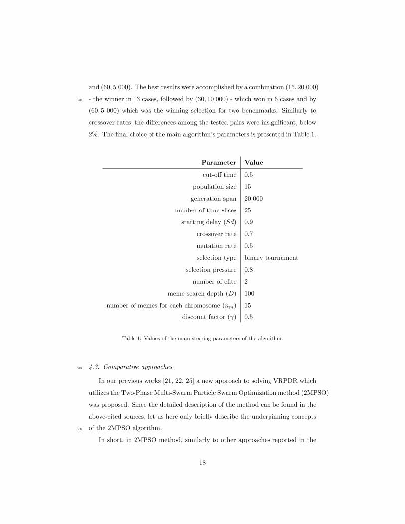
2%. The final choice of the main algorithm’s parameters is presented in Table 1.

Parameter Value

cut-off time 0.5

population size 15

generation span 20 000

number of time slices 25

starting delay (Sd) 0.9

crossover rate 0.7

mutation rate 0.5

selection type binary tournament

selection pressure 0.8

number of elite 2

meme search depth (D) 100

number of memes for each chromosome (nm) 15

discount factor (γ) 0.5

Table 1: Values of the main steering parameters of the algorithm.

4.3. Comparative approaches375

In our previous works [21, 22, 25] a new approach to solving VRPDR which

utilizes the Two-Phase Multi-Swarm Particle Swarm Optimization method (2MPSO)

was proposed. Since the detailed description of the method can be found in the

above-cited sources, let us here only briefly describe the underpinning concepts

of the 2MPSO algorithm.380

In short, in 2MPSO method, similarly to other approaches reported in the

18

literature, the working day is divided into some number of time slices and in

each of them a currently available instance of the (static) VRP is solved. What

accounts for the main difference between 2MPSO and majority of the CI-based

approaches described in the literature is that in each time slice the solving385

process of 2MPSO is split into two separate phases: a clustering phase (i.e.

assignment of requests to vehicles) and optimization phase (i.e. route construc-

tion for each of the vehicles). Each of these two above-mentioned subproblems

is solved by a separate multi-swarm PSO system. One of the key features of the

2MPSO is effective knowledge transfer between multiple swarms (in-phase) and390

between swarms used in consecutive time slices.

In the first phase each particle is represented as a real number vector whose

elements denote centers of clusters of requests assigned to vehicles. The area of

clients’ requests is divided among vehicles on the basis of the Euclidean distances

from the client’s location to the clusters’ centers (i.e. a request is assigned to a395

vehicle which serves the nearest cluster).

In the second phase each particle represents the order of requests assigned to

a given vehicle (each cluster/vehicle is solved by a separate PSO instance). The

order is obtained by sorting particles’ coordinates in the ascending order. The

solution assessment in the second phase (in each of the PSO instances) is equal400

to the length of a route (of a given vehicle) defined by the proposed ordering.

The final cost value is equal to the sum of the assessments of the best solutions

found by each of the PSO instances.

In [22] the 2MPSO algorithm was extensively compared with several population-

based methods, namely the Ant Colony Optimization [19], evolutionary ap-405

proach [20], Tabu Search [20] and another, well-established in the literature,

PSO-based approach: MEMSO/MAPSO [24, 23, 34] by Khouadija et al. The

tests were performed on the same set of benchmarks as those used in this work,

described in section 4.1.

On a general note, the extensive experimental comparison proved an upper410

hand of the 2MPSO approach, which for comparable (≈ 107) number of fitness

function evaluations was capable of finding new best literature solutions in 11

19

out of 21 test instances. In terms of the average results the 2MPSO outper-

formed the competitive methods by at least 1.5%. For the sake of clarity of the

presentation the experimental results and conclusions drawn in [22] are not re-415

peated in detail here. Due to the superiority of 2MPSO over all the above-listed

metaheuristic approaches we will use this method as a reference point to our

memetic VRPDR algorithm (M-VRPDR).

5. Experimental results

One of the most universal complexity measures of population-based methods420

is the number of fitness function evaluations (FFE) of the candidate solutions.

This measure allows for making (rough) comparisons between various GA/EA

approaches as well as Particle Swarm Optimization or Tabu Search methods. In

our method the fitness evaluation is performed in three parts of the algorithm:

in crossover operation (in order to find the best position in a chromosome for425

insertion of removed customer), in selection (so as to choose better-fitted chro-

mosomes for the next generation) and in memetic optimization (to check how

the meme operation affects the cumulative length of the vehicle routes). In all

baseline numerical results presented in this section the number of FFE in a sin-

gle algorithm’s run is close to (but never exceeds) 107, which is the value used430

to calculate the main results obtained in [22] for other methods.

Results of experiments with steering parameters set according to Table 1

are presented in Tables 2, 3 and 5. The first table shows the best result and

the average result out of 50 independent trials for each of the 21 benchmark

sets of our M-VRPDR approach and the 2MPSO method (in both cases with435

a budget of 107 FFE). In terms of the ability to find the best possible solution

(Min category comparison) M-VRPDR outperforms 2MPSO by a large margin

- winning in 17 benchmarks and losing in 4 cases. In particular, M-VRPDR

proved to be better suited for all Taillard’s benchmarks.

When comparing the average performance, which in practice is usually more440

desirable, as it addresses the issue of repeatability and stability of results the

20

advantage of M-VRPDR is not so prevailing, though the method yielded better

averages in 14 test sets, losing in the remaining 7. The memetic approach

again showed its upper-hand in the case of Taillard’s instances. The difference

in average results between the two methods is statistically significant for p −445

value = 0.007 for 1-tailed t-test for averages and p− value = 0.015 for 2-tailed

t-test.

Table 3 compares the best results of M-VRPDR with those found in the

literature (including the results of 2MPSO). Both results are attained with the

same number of FFE. Our method found the new best literature results in 14450

cases.

A more detailed results, including the worst outcomes and standard devia-

tions of the 50 tests with M-VRPDR for each of the benchmarks, as well as the

exemplar convergence graphs for the sets c100bd and tai150aD are presented in

Appendix A.455

5.1. Hard cases for the M-VRPDR

Based on the average results presented in Table 2 it can be noticed that

the algorithm does not manage equally well for all benchmarks. The worst

average results compared to 2MPSO were achieved for instances c100bD and

c120D. In these two problems distributions of clients’ locations have the form460

of highly-spatial clusters composed of uniformly distributed request sizes. Fig-

ures 8 and 9 show the routes proposed by our algorithm for c100bD and c120D

benchmarks. In both presented solutions there exist routes which include re-

quests from two different clustered groups of clients which elongate the overall

solution (if these clusters were served by different vehicles the solutions might465

be shorter). According to our intuition such a behavior can be attributed to

the vehicles’ starting delay. The imposed condition that a vehicle can move

to a customer only if a planned return time to the depot exceeds 90% of the

working day’s span causes the planned routes to be relatively long so as to ex-

tend routing time beyond the assumed part of the working day. In the case of470

clustered clients it might potentially be more efficient to serve only one cluster

21

Figure 8: Route networks for instance c100bD.

Figure 9: Route networks for instance c120D.

22

M-VRPDR (107) 2MPSO (107)

Min Avg Min Avg

c50D 524.61 548.10 552.47 591.29

c75D 852.95 885.00 878.93 904.12

c100D 860.56 913.81 874.20 920.84

c100bD 820.92 864.03 819.56 839.01

c120D 1189.06 1295.31 1056.28 1131.30

c150D 1083.79 1142.24 1096.53 1131.78

c199D 1377.26 1466.30 1362.84 1415.58

f71D 260.17 297.61 282.69 291.61

f134D 11815.95 12299.59 11755.58 12038.28

tai75aD 1656.12 1705.76 1682.90 1766.68

tai75bD 1350.28 1378.47 1404.29 1447.30

tai75cD 1355.41 1427.74 1406.59 1498.18

tai75dD 1376.42 1414.93 1415.79 1439.78

tai100aD 2093.63 2168.87 2155.42 2215.44

tai100bD 1990.99 2097.86 2022.13 2102.15

tai100cD 1421.50 1460.72 1446.10 1493.59

tai100dD 1631.63 1710.44 1690.32 1753.17

tai150aD 3226.51 3354.09 3298.91 3394.92

tai150bD 2847.08 2980.33 2887.88 2992.81

tai150cD 2427.53 2558.99 2462.96 2551.58

tai150dD 2737.37 2903.68 2886.12 2941.66

Table 2: The best and the average results of M − V RPDR(107) and 2MPSO(107) for the

considered benchmarks. The better of the two results in each category (Min, Avg) is bolded.

of clients per vehicle and return to the depot immediately after, regardless of

the time of a day and available capacity left. In order to verify this hypoth-

esis, 50 tests were performed for these two benchmarks with Sd times set to

23

M-VRPDR Best other Algorithm #FFE

c50D 524.61 552.47 2MPSO3 [22] 107

c75D 866.45 877.30 2MPSO2 [22] 2 · 106

c100D 873.10 874.20 2MPSO3 [22] 108

c100bD 820.92 819.56 2MPSO3 [22] 108

c120D 1199.64 1056.28 2MPSO3 [22] 108

c150D 1083.79 1096.53 2MPSO3 [22] 107

c199D 1376.26 1362.84 2MPSO3 [22] 108

f71D 275.51 278.65 2MPSO3 [22] 105

f134D 11817.66 11755.58 2MPSO3 [22] 108

tai75aD 1658.13 1682.90 2MPSO3 [22] 108

tai75bD 1351.06 1391.74 2MPSO3 [22] 2.2 · 107

tai75cD 1388.13 1406.27 TabuSearch [20] 25 · 30sec

tai75dD 1395.30 1342.26 MEMSO [23] 106

tai100aD 2122.92 2146.53 2MPSO2 [22] 2.2 · 107

tai100bD 1990.99 2022.13 2MPSO3 [22] 107

tai100cD 1419.89 1446.10 2MPSO3 [22] 108

tai100dD 1651.28 1685.53 2MPSO2 [22] 2.2 · 107

tai150aD 3343.54 3253.77 MEMSO [23] 106

tai150bD 2957.16 2861.91 MAPSO [34] 106

tai150cD 2430.91 2462.96 2MPSO3 [22] 108

tai150dD 2742.35 2844.70 2MPSO2 [22] 2.2 · 107

Table 3: Comparison of the best M-VRPDR results (2nd column) with the hitherto best-

known literature solutions (3rd column) accomplished by the algorithm presented in the 4th

column. Both results are attained with the same number of FFE (5th column) - defined in the

cited papers. In one case (tai75cD), following [20], instead of the number of FFE, the time

measure is used for methods’ comparison. For each benchmark the better outcome is bolded.

24

0.0, 0.05, 0.1, 0.15, . . . , 0.85 hoping that the possibility to start the route earlier475

would alleviate the problem of ineffective (packed close to the capacity limit)

routes. Unfortunately, all these values appeared to be weaker choices than 0.9

- the setting used in the main experiment. The main reason for that is a large

number of trucks which are at the algorithm’s disposal (in all tested benchmarks

this limit is set to 50, which is well beyond the practical needs). Having suffi-480

cient number of spare vehicles there is no real need for any truck to optimize its

route in a way which would allow the vehicle to make two tours within a day.

Consequently, the trucks were leaving depot earlier than in the main experiment

but at the same time were much more “careless” about the route optimization,

having enough time and capacity to extend the solution in different ways. It485

seems that the case of densely clustered customers’ distributions requires special

attention and we have put this issue on the top of our priority list.

Furthermore, visibly worse results were also obtained for benchmarks c150D

and c199D. While we could not trace any specific attributes of these sets other

than their size, we hypothesized that the number of iterations might have been490

too small to allow the convergence to a good solution due to the higher (than in

other cases) number of customers. In order to verify this claim, we performed

additional tests for all four “resistant” benchmarks: c100bD, c120D, c150D,

c199D with doubled number of iterations. The results are presented in Table 4.

In the case of bigger benchmark sets (c150D and c199D) the results improved by495

about 2.5% which seems to confirm our presumption. For the densely clustered

problems, however, the improvement is meaningless, about 1%.

6. Saliency of the memetic component

While encouraging experimental results, in particular the ability to find new

best literature results for a bunch of popular and widely-recognizable bench-500

marks, give prospects for possible applicability and further development of the

M-VRPDR, from the research point of view the most pertinent question is re-

lated to the reasons of such a promising behavior.

25

M-VRPDR with

doubled iterations M-VRPDR

Min Avg Min Avg

c100bD 819.56 855.74 820.92 864.03

c120D 1192.35 1282.27 1189.06 1295.31

c150D 1071.78 1112.12 1083.79 1142.24

c199D 1365.26 1430.52 1377.26 1466.30

Table 4: Result of the algorithm with doubled numbers of iterations for 4 benchmarks for

which M-VRPDR obtained the worst results.

Based on some number of preliminary tests it turned out that in the parametriza-

tion layer the crucial variable is the starting delay parameter, whose proper505

setting is indispensable for efficient solving of VRPDR. In order to deeper in-

vestigate this issue additional tests were performed aiming at comparison of the

“pure” genetic approach (i.e. without memetic optimization) without consider-

ing the starting delay parameter, the pure genetic approach with starting delay

value set to 0.9 (as in the main experiment) and the M-VRPDR. The lack of510

memetic optimization phase in both purely genetic implementations was com-

pensated by the increased number of iterations, so as to maintain approximately

the same number of FFE.

Table 5 presents comparison of results obtained by M-VRPDR and the two

genetic approaches (with and without considering the Sd parameter) based on515

50 independent runs in each case. The importance of both tested factors (start-

ing delay parameter and memetic optimization) is clearly supported by the

results. The purely GA approach, without taking into account Sd factor, was

not a competitive approach for any of the considered benchmarks. In average it

yielded the solution 11.18% longer than those of the same GA implementation520

which relied on the starting delay. This enhanced GA approach incidentally

appeared to be stronger than M-VRPDR in terms of best-found solution, but

in a more systematic measure, by means of the average solution length, it lost

26

GA-Sd GA+Sd M-VRPDR

Min Avg Min Avg Min Avg

c50D 598.86 634.86 527.17 566.25 524.61 548.10

c75D 984.83 1059.16 865.70 898.40 852.95 885.00

c100D 1004.36 1061.87 868.94 940.20 860.56 913.81

c100bD 880.19 996.82 824.94 884.56 820.92 864.03

c120D 1282.32 1474.45 1222.00 1421.14 1189.06 1295.31

c150D 1377.09 1480.56 1089.41 1176.25 1083.79 1142.24

c199D 1762.94 1888.07 1436.00 1506.24 1377.26 1466.30

f71D 279.02 304.48 274.02 304.24 260.17 297.61

f134D 15480.35 16309.51 11795.55 12711.37 11815.95 12299.59

tai75aD 1758.56 1866.33 1668.75 1735.95 1656.12 1705.76

tai75bD 1480.91 1603.10 1352.04 1382.08 1350.28 1378.47

tai75cD 1516.50 1604.15 1372.42 1456.85 1355.41 1427.74

tai75dD 1456.45 1561.61 1393.19 1424.66 1376.42 1414.93

tai100aD 2185.52 2377.83 2103.70 2193.21 2093.63 2168.87

tai100bD 2136.29 2321.65 2049.49 2141.61 1990.99 2097.86

tai100cD 1564.66 1670.13 1425.17 1475.23 1421.50 1460.72

tai100dD 1801.75 1943.67 1661.63 1742.45 1631.63 1710.44

tai150aD 3541.84 3858.63 3241.59 3409.37 3226.51 3354.09

tai150bD 3109.13 3469.71 2845.46 3076.60 2847.08 2980.33

tai150cD 2738.08 2989.05 2442.11 2643.10 2427.53 2558.99

tai150dD 3055.80 3238.90 2810.29 2958.12 2737.37 2903.68

Table 5: Comparison of results obtained by M-VRPDR and the two genetic approaches (with

and without considering the Sd parameter, denoted by GA+Sd and GA-Sd, respectively)

based on 50 independent runs with a budget of 107 FFE in each case. Best results are bolded.

to M-VRPDR in all cases, with the average margin of 2.47%.

27

7. Summary and conclusions525

This paper presents a memetic approach to solving the Vehicle Routing Prob-

lem with Dynamic Requests. The algorithm was tested on a well-established

set of benchmarks and proved to be an effective and reliable method, capable

of finding 13 new best-known results out of 21 tested problems, using the same

numbers of fitness function evaluations. It is worth underlying that, except for530

some parameter tuning, the method was not optimized for solving this particu-

lar set of benchmarks. Furthermore, the proposed algorithm can, in principle,

be applied to solving other VRPDR benchmarks with no specific adjustments

as the selected parameters seem to be universally useful (though certainly not

optimal in strict sense).535

Our algorithm relies on problem encoding previously introduced in [20] and

adopts memetic optimization scheme proposed in [9], however, both these fac-

tors are combined in a novel manner as parts of the newly-designed system

and applied to the problem other that those considered in the source papers.

Furthermore, while memetic optimization is definitely an important part of the540

overall solution method, the paramount feature is the starting delay parameter

which heuristically administers the dispatching times of the vehicles.

Additionally, a new way of knowledge transfer between consecutive partial

solutions defined during the day (in subsequent time-slices) is introduced in this

study and proved to be effective when combined with the proposed extensive545

mutation operator which prevents the system from premature convergence or

stagnation.

Our current research focus is on development of a meta-heuristic procedure,

which - based on the analysis of particular data set (spatial and volume dis-

tributions of requests, their skewness and approximate number of clusters) -550

would autonomously adjust the parameters of the method so as to increase its

efficacy in solving a given benchmark set. Such a meta-heuristic system can, for

instance, be implemented as a one-layer feed-forward network and trained on an

ensemble of benchmarks, taking the statistical parameters of the data set as in-

28

puts. Special focus will be put on the case of densely clustered data sets, which555

appeared to be the most demanding for the current system implementation. We

hope that due to intrinsic nonlinearity of neural networks’ approximation the

proposed meta-approach will further strengthen the system’s performance.

Acknowledgment

The research was financed by the National Science Centre in Poland, grant560

number DEC-2012/07/B/ST6/01527. The authors would like to thank Micha l

Okulewicz for his helpful comments.

Appendix A

The appendix presents statistical characteristics of the baseline M-VRPDR

(107) results (Table 6) and two exemplar convergence graphs (Figures 10 and 11),565

respectively for c100bD and tai150aD benchmark sets.

The results presented in Table 6 show that the method is reliable (repeat-

able), as for all benchmarks the standard deviation is kept within reasonable

limits compared to the average solution. The greatest spread of outcomes (in

per cent points) can be observed for f71D (4.79%) and tai150cD (4.09%), while570

the most consistent results are obtained in the case of f134D (only 1.46%) and

tai75bD (1.51%). Overall, the worst solutions (column Max) are within the

11.21% margin (achieved for tai150aD) from the average results across all bench-

marks, but can be as low as 3.01% for f134D or 3.43% for tai75bD.

References575

[1] G. B. Dantzig, R. Ramser, The Truck Dispatching Problem, Management

Science 6 (1959) 80–91.

[2] L. M. Gambardella, ric Taillard, G. Agazzi, Macs-vrptw: A multiple ant

colony system for vehicle routing problems with time windows, in: New

Ideas in Optimization, McGraw-Hill, 1999, pp. 63–76.580

29

Figure 10: The convergence graphs for 12 independent algorithm’s runs for the c100bD bench-

mark set. The x-axis represents time (time slices) and the y-axis - the length of the currently

committed tour. It can be seen from the figure that the experiments are fairly repeatable.

After the cut-off time (time slice #13) only local route optimization takes place.

Figure 11: The convergence graphs for 12 independent algorithm’s runs for the tai150aD

benchmark set. The x-axis represents time (time slices) and the y-axis - the length of the

currently committed tour. It can be seen from the figure that the experiments are fairly

repeatable. After the cut-off time (time slice #13) only local route optimization takes place.

30

Min Avg Max St dev St dev/Avg

c50D 524.61 548.10 582.09 17.49 3.19%

c75D 852.95 885.00 944.83 22.14 2.50%

c100D 860.56 913.81 999.41 29.98 3.28%

c100bD 820.92 864.03 927.51 25.93 3.00%

c120D 1189.06 1295.31 1407.31 49.67 3.83%

c150D 1083.79 1142.24 1234.75 38.18 3.34%

c199D 1377.26 1466.30 1596.62 45.08 3.07%

f71D 260.17 297.61 324.61 14.25 4.79%

f134D 11815.95 12299.59 12669.69 180.06 1.46%

tai75aD 1656.12 1705.76 1797.22 34.22 2.01%

tai75bD 1350.28 1378.47 1425.69 20.88 1.51%

tai75cD 1355.41 1427.74 1538.73 37.90 2.65%

tai75dD 1376.42 1414.93 1481.04 24.23 1.71%

tai100aD 2093.63 2168.87 2357.59 53.48 2.47%

tai100bD 1990.99 2097.86 2195.63 55.92 2.67%

tai100cD 1421.50 1460.72 1564.04 31.02 2.12%

tai100dD 1631.63 1710.44 1820.74 49.64 2.90%

tai150aD 3226.51 3354.09 3730.07 106.00 3.16%

tai150bD 2847.08 2980.33 3134.90 74.73 2.51%

tai150cD 2427.53 2558.99 2828.03 104.55 4.09%

tai150dD 2737.37 2903.68 3063.57 67.63 2.33%

Table 6: Detailed results of the M-VRPDR method for all 21 benchmarks with a budget of

107 FFE in each test.

[3] A. H. Michel Gendreau, G. Laporte, A tabu search heuristic for the vehicle

routing problem, Management Science 40 (10) (1994) 276–1290.

[4] Y. Wu, P. Ji, T. Wang, An empirical study of a pure genetic algorithm

to solve the capacitated vehicle routing problem, ICIC Express Letters 2

31

(2008) 41–45.585

[5] I. H. Osman, Metastrategy simulated annealing and tabu search algorithms

for the vehicle routing problem, Annals of Operations Research 41 (4)

(1993) 421–451.

[6] J. Mandziuk, C. Nejman, UCT-based approach to Capacitated Vehicle

Routing Problem, in: Artificial Intelligence and Soft Computing, Vol. 9120590

of Lecture Notes in Computer Science, Springer Berlin Heidelberg, 2015,

pp. 679–690.

[7] N. Wilson, N. Colvin, Computer control of the rochester dial-a-ride sys-

tem, Tech. Rep. R77-31, Departament of Civil Engineering, Massachusetts

Institute of Technology, Cambridge, Massachusetts.595

[8] P. Kilby, P. Prosser, P. Shaw, Dynamic VRPs: A Study of Scenarios, ac-

cessed: 2015-09-01 (1998).

URL http://www.cs.strath.ac.uk/~apes/apereports.html

[9] X. Chen, L. Feng, Y. Ong, A self-adaptive memeplexes robust search

scheme for solving stochastic demands vehicle routing problem, Int. J. Sys-600

tems Science 43 (7) (2012) 1347–1366.

[10] L. Wen, B. atay, R. Eglese, Finding a minimum cost path between a pair of

nodes in a time-varying road network with a congestion charge, European

Journal of Operational Research 236 (3) (2014) 915 – 923.

[11] J. Mandziuk, M. Swiechowski, UCT method in stochastic transportation605

problems, accessed: 2015-09-01 (Unpublished results).

URL http://www.mini.pw.edu.pl/~mandziuk/WORK/UCT-DVRP.pdf

[12] D. Tas, M. Gendreau, N. Dellaert, T. van Woensel, A. de Kok, Vehicle

routing with soft time windows and stochastic travel times: A column

generation and branch-and-price solution approach, European Journal of610

Operational Research 236 (3) (2014) 789 – 799.

32

[13] D. Cattaruzza, N. Absi, D. Feillet, T. Vidal, A memetic algorithm for

the multi trip vehicle routing problem, European Journal of Operational

Research 236 (3) (2014) 833 – 848.

[14] M. M. Abdulkader, Y. Gajpal, T. Y. ElMekkawy, Hybridized ant colony615

algorithm for the multi compartment vehicle routing problem, Applied Soft

Computing 37 (2015) 196 – 203.

[15] K. Ghoseiri, S. F. Ghannadpour, Multi-objective vehicle routing problem

with time windows using goal programming and genetic algorithm, Appl.

Soft Comput. 10 (4) (2010) 1096–1107.620

[16] R. Masson, S. Ropke, F. Lehud, O. Pton, A branch-and-cut-and-price ap-

proach for the pickup and delivery problem with shuttle routes, European

Journal of Operational Research 236 (3) (2014) 849 – 862.

[17] P. Toth, D. Vigo, Special issue on vehicle routing and distribution logistics,

European Journal of Operational Research 236 (3) (2014) IFC –.625

[18] B. Eksioglu, A. V. Vural, A. Reisman, The vehicle routing problem: a

taxonomic review, Computers & Industrial Engineering 57 (4) (2009) 1472

– 1483.

[19] R. Montemanni, L. Gambardella, A. Rizzoli, A. Donati, A new algorithm

for a dynamic vehicle routing problem based on ant colony system, Journal630

of Combinatorial Optimization 10 (2005) 327–343.

[20] F. T. Hanshar, B. M. Ombuki-Berman, Dynamic vehicle routing using

genetic algorithms, Applied Intelligence 27 (1) (2007) 89–99.

[21] M. Okulewicz, J. Mandziuk, Application of Particle Swarm Optimization

Algorithm to Dynamic Vehicle Routing Problem, in: Artificial Intelligence635

and Soft Computing, Vol. 7895 of Lecture Notes in Computer Science,

Springer Berlin Heidelberg, 2013, pp. 547–558.

33

[22] M. Okulewicz, J. Mandziuk, A two-phase multi-swarm algorithm for solv-

ing dynamic vehicle routing problem, accessed: 2015-09-01 (Unpublished

results).640

URL http://www.mini.pw.edu.pl/~mandziuk/WORK/2MPSO.pdf

[23] M. R. Khouadjia, E.-G. Talbi, L. Jourdan, B. Sarasola, E. Alba, Multi-

environmental cooperative parallel metaheuristics for solving dynamic op-

timization problems, Journal of Supercomputing 63 (3) (2013) 836–853.

[24] M. R. Khouadjia, B. Sarasola, E. Alba, L. Jourdan, E.-G. Talbi, A com-645

parative study between dynamic adapted PSO and VNS for the vehicle

routing problem with dynamic requests, Applied Soft Computing 12 (4)

(2012) 1426–1439.

[25] J. Mandziuk, S. Zadrozny, K. Waledzik, M. Okulewicz, M. Swiechowski,

Adaptive metaheuristic methods in dynamically changing environments,650

accessed: 2015-09-01 (2015).

URL http://www.mini.pw.edu.pl/~mandziuk/dynamic/

[26] Y. S. Ong, M. H. Lim, X. S. Chen, Research frontier: Memetic computation

- past, present & future, IEEE Computational Intelligence Magazine 5 (2)

(2010) 24–36.655

[27] X. S. Chen, Y. S. Ong, M. H. Lim, K. C. Tan, A multi-facet survey on

memetic computation, IEEE Transactions on Evolutionary Computation

15 (5) (2011) 591–607.

[28] F. Neri, C. Cotta, Memetic algorithms and memetic computing optimiza-

tion: A literature review, Swarm and Evolutionary Computation 2 (2012)660

1–14.

[29] A. K. Raymond Kwan, A. Wren, Evolutionary driver scheduling with relief

chains, Evolutionary Computation 9 (4) (2001) 445–460.

34

[30] X. Chen, Y. Ong, M. H. Lim, Cooperating memes for vehicle routing prob-

lems, International Journal of Innovative Computing, Information and Con-665

trol 7 (2011) 1–10.

[31] N. Christofides, J. E. Beasley, The period routing problem, Networks 14 (2)

(1984) 237–256.

[32] M. L. Fisher, R. Jaikumar, A generalized assignment heuristic for vehicle

routing, Networks 11 (2) (1981) 109–124.670

[33] E. D. Taillard, Parallel iterative search methods for vehicle routing prob-

lems, Networks 23 (8) (1993) 661–673.

[34] M. R. Khouadjia, E. Alba, L. Jourdan, E.-G. Talbi, Multi-Swarm Optimiza-

tion for Dynamic Combinatorial Problems: A Case Study on Dynamic Ve-

hicle Routing Problem, in: Swarm Intelligence, Vol. 6234 of Lecture Notes675

in Computer Science, Springer, Berlin / Heidelberg, 2010, pp. 227–238.

35

Vitae

Jacek Mandziuk PhD, DSc. is Associate Professor

at Faculty of Mathematics and Information Science, War-

saw University of Technology, Head of Division of Arti-680

ficial Intelligence and Computational Methods and Head

of Doctoral Programme in Computer Science. In 2011 he

was awarded the title of Professor Titular.

He is the author of 3 books and 100+ research pa-

pers, an Associate Editor of several journals including685

IEEE Transactions on Computational Intelligence and AI

in Games. He is a recipient of the Senior Fulbright Advanced Research Award.

His research interests include application of CI to games, dynamic opti-

mization, human-machine cooperation, financial modeling, and development of

general-purpose human-like learning and problem-solving methods which in-690

volve intuition, creativity and multitasking.

Adam Zychowski received his B.Sc. and M.Sc. de-

grees in Computer Science from the Faculty of Mathemat-

ics and Information Science, Warsaw University of Tech-

nology, Warsaw, Poland in 2014 and 2015, respectively.695

His research interests include Computational Intelli-

gence methods and their application to solving complex,

real-life problems.

36