a markov switching unobserved component analysis of … · 2014-10-22 · a markov switching...
TRANSCRIPT
A Markov Switching Unobserved Component Analysis of the
CDX Index Term Premium
Giovanni Calice
*1, Christos Ioannidis
**, RongHui Miao
***
Abstract
Using a Markov switching unobserved component model we decompose the term premium of
the North American CDX investment grade index (CDX-IG) into a permanent and a
stationary component. We explain the evolution of the two components in relating them to
monetary policy and stock market variables. We establish that the inversion of the CDX
index term premium is induced by sudden changes in the unobserved stationary component,
which represents the evolution of the fundamentals underpinning the probability of default in
the economy. We find strong evidence that the unprecedented monetary policy response from
the Fed during the 2008-2009 financial crisis period was effective in reducing market
uncertainty and helped to steepen the term structure of the index thereby mitigating systemic
risk concerns. The impact of stock market volatility, as captured by the VIX index, in
flattening the term premium was substantially more robust in the crisis period. We also show
that equity returns make a substantial contribution to the term premium over the entire sample
period.
1 We are grateful to Viral Acharya, Darrel Duffie, Jorge Antonio Chan-Lau (Discussant), Nicolas Dubourg
(Discussant), Alexander Karmann (Discussant), Francis Longstaff and three anonymous referees for their
suggestions as well as seminar participants at the International Monetary Fund, Bank for International
Settlements, Bank of England, Bank of Finland, Central Bank of Spain, Bank of Korea, Central Bank of Turkey,
University of Bath, University of Durham, Bilkent University, National University of Singapore (NUS),
Australian National University (ANU, Canberra), Barclays Capital, FitchRatings, Goldman Sachs, J.P. Morgan,
Morgan Stanley (New York), the Deutsche Bundesbank, Technische Universität Dresden and Journal of
Financial Stability Conference on "The Stability of the European Financial System and the Real Economy in the
Shadow of the Crisis" (Dresden) , the DIW Berlin Conference on the “Role of Finance in Stabilizing the Past,
Present, and Future Real Economy” (Berlin), the 4th Financial Risks International Forum (Paris), the 8th
Annual Conference of Asia-Pacific Association of Derivatives (Busan, Korea), Central Bank of the Republic of
Turkey Conference on “Financial and Macroeconomic Stability: Challenges Ahead” (Istanbul) for their
comments. A part of this work was conducted while Giovanni Calice was visiting ANU, the Bank of Finland
and New York University (NYU). We are indebted to Ashley Musfeldt and Morgan Stanley (New York) for
sharing data with us. All errors are our responsability.
*Corresponding author. University of Birmingham, Department of Economics, Edgbaston, Birmingham,
B152TT. E-mail: [email protected]
Tel: +44 (0) 121 414 4956. Fax: +44 (0) 121 414 7377.
** University of Bath, Claverton Down, BA2 7AY, Bath. E-mail: [email protected].
*** Aviva plc., St. Helen’s, 1 Undershaft, London, EC3P3DQ. E-mail: [email protected].

2
First Draft: July 2011. Current Version: August 2014
JEL Classification: G01, G15, G21, G24
Keywords: CDX Index, Markov Switching, State-Space, Variance Decomposition, Term
Premium

3
1. Introduction
The sub-prime mortgage crisis, unveiled in July 2007, has caused billions of dollars
of losses in the credit markets as systemically important financial institutions had been forced
to write off mortgages and related securities linked to credit derivatives instruments, like
credit default swaps (CDSs) and collateralized debt obligations (CDOs). Great uncertainties
filled almost every corner of the financial markets, which seriously interrupted its normal
functioning (see Taylor and Williams (2008)).
It has been argued (see, amongst the others, Longstaff (2010), Calice (2011)) that the
2007/2008 sub-prime crisis was amplified through structured credit products-tranches
trading. Consequently, if on the one hand, these instruments seem to have enriched the scope
of investment strategies, on the other hand, their increased complexity depth have unduly
induced instability in financial markets.
CDS indices are simply portfolios of single name default swaps, serving both as
trading vehicles and as barometers of credit market conditions. Users of the most popular
indices (the Dow Jones CDX North American investment grade and the iTraxx Europe
investment grade) include those who want to hedge against credit defaults of pooled entities
and those who want to speculate.
These indices are responsible for the increased liquidity and popularity of tranching
of credit risk. By buying protection on an index, an investor is protected against defaults in
the underlying portfolio and makes quarterly premium payments to the protection seller. If
there is a default, the protection seller pays par to the protection buyer.
The term premium of the CDX index which, in this paper, is measured as the
difference between the CDX 10-year and the CDX 5-year maturities, can be viewed as
representing the uncertainty regarding corporate default over a 5 years time horizon.
Therefore, the CDX term premium can be interpreted as an early warning market indicator of
improvement or deterioration in macroeconomic conditions for the next 5 years.
If an investor perceives the difference between the 5-year index premia and the 10-
year index premia too steep, in other words, that the implied probability of default between 5
and 10 years is higher than that implied from fundamentals, but he/she expects the slope to
flatten, then this investor could buy 5-year protection and sell 10-year protection on the CDX
index. Finance theory suggests that the credit curves of companies with high credit quality
should be upward sloping, whereas those of companies having very poor credit quality do
exhibit negative slopes. For example, the credit risk of an AAA rated corporate bond should
4
in general be positively correlated with its maturity, and hence the required yields slope
upwards against its maturity. In cross-sectional space, the likelihood of credit quality
deterioration should increase as rating lowers, which is to say that the required average yield
should increase with the downgrading of corporate bonds. However, the credit curve for a
company on the brink of default (or with foreseeable immediate downgrade) would invert to
trend negatively to reflect higher credit risk in the near future. As a result, the yield for such
bond is very high for short maturities but relatively lower for longer maturities, which reflects
investors’ view that it is still possible for this company to improve its credit quality for longer
term maturities.
CDX curve trading has assumed enormous importance over the latest very turbulent
period. Clearly, curves tend to flatten in periods of imminent higher default rates, and tend to
be steep in periods of economic expansion.
Index curve trading is generally motivated on one or more of the following2
a) As a way of expressing market direction views with different risk-reward profiles.
b) Carry and roll-down reasons.
c) Hedging purposes – both cash and CDS underlying portfolios.
Many opportunities for trading curves on single-name CDS occur around forecasted
or announced specific corporate actions. Such events change the perception of a company’s
creditworthiness and the shape of the CDS curve also evolves. Curve trades can be more
attractive than outright positions around events, thanks to the variation in the available payoff
profiles.
In addition, macroeconomic conditions can trigger default events that affect the
curves of not only specific entities but also of entire industries. Changes in consumer
preferences, the monetary policy stance, and developments in the housing market are critical
industry-wide events and market sentiment often transcend worries about profitability and
focus instead on viability and the possibility of default of a specific firm. In this case,
recovery expectations, following a higher default rate regime, become progressively
important in determining the curve shape of the index, as it clearly tends to flatten.
In this paper, we investigate the dynamic behaviour of the CDX index term premium,
the difference between the 10-year and 5-year maturities, through time by using a Markov
Switching Unobserved Component (MS-UC) model. In the econometric literature, several
approaches have been proposed on the decomposition of univariate time series. A well-
2 For more details, see Barclays Capital Research (2008), "CDS Curve Trading Handbook 2008".

5
established methodology is the unobserved components approach, postulated in separate
contributions by Harvey (1985), Watson (1986) and Clark (1987), respectively. It seems
natural to consider an economic time series in terms of permanent and stationary components.
The decomposition of a univariate time series into these two components is a primary tool for
analyzing business cycles, with these two components often used as measurements of
unobserved trend and cycle. Traditionally researchers also adopted unobserved component
models to study mean reversion in stock prices. Fama and French (1988) find a stationary
mean reverting component in addition to a permanent component in the US stock price
dynamics. Porterba and Summers (1988) test the existence of a stationary component
although they do not perform a formal decomposition of the stock prices in stationary and
permanent components. Others like Lo and McKinlay (1988) and Kim et al. (1991) use
variance ratio tests to detect mean reversion in stock prices. Although the evidence of mean
reversion in stock prices is mixed, as Summers (1986) argues, statistical tests used in testing
the random walk (RW) hypothesis have usually low power against the alternative of mean
reversion.
In formulating an unobserved components model for econometric analysis, we depart
from others working on the observable determinants of CDS indices. Alexander and Kaeck
(2008) and Byström (2006), for example, relate the CDS/CDX premia to several observed
variables (such as the slope of the yield curve, stock market returns and stock market
volatility), and analyze the significance of each observable variable in determining the CDS
iTraxx Europe premia using single-equation regression. Our interest in this paper, however, is
to study how the factors themselves (not the factor loadings) drive the dynamics of the term
premium. Since the CDX index measures the economy-wide default probabilities (the higher
the index value, the higher the probability of default on firms included in the index), the
macroeconomic conditions, which can be encompassed by those fundamental factors, will be
closely related to the CDX index value and its term premium.
To characterize the observed patterns of volatility jumps on the CDX index term
premium, we allow on the innovation terms a regime switching process, following two
distinct first-order Markov chain variables.
This paper contributes to the rapidly growing literature on structured credit in its
attempt to understand the evolution of the term premium of the CDS index market and its link
to observed macroeconomic and financial information.
Our paper has two main contributions. First, we present a readily implementable new
approach to modeling CDS index dynamics, by conducting a regime dependent factor

6
analysis of the evolution of the CDX index. Second, we provide insights into how the
fundamental and volatility components of the CDX index are determined by daily observed
monetary policy and stock market variables, over a sample period surrounding the 2007-2009
global financial crisis.
The current literature on CDS is primarily limited to the pricing with a large strand of
it revolving around the key determinants of these contracts. First, there is an extensive
literature on the driving forces of CDS premia ranging from the model of Hull, Predescu and
White (2004), Aunon-Nerin, Cossin, Hricko and Huang (2002), which examine the
relationship between CDS premia and credit spreads, to more elaborate analysis by – amongst
the others – Zhu (2006), Longstaff, Mithal and Neis (2005) and Blanco, Brennan and Marsh
(2005) which include also bond and equity markets measures.
Much of the research on credit markets has focused on corporate bond spreads and
single-name CDS premia. Despite a sizeable literature on credit risk empirical studies on
CDS that involve the modeling of the entire credit curve are uncommon. A major reason for
this is that data on the CDS premia for a wide range of maturities have only recently become
available. Consequently there is a paucity of empirical works regarding CDS indices, with
studies focused mainly on the North America CDX investment grade index (CDX.NA.IG).
Our work is also closely related to two recent studies by Pan and Singleton (2008)
and Zhang (2008), who attempt to estimate default risk using the entire credit curve of
sovereign CDS premia. Byström (2005, 2006) and Alexander and Kaeck (2008) are the early
studies on CDS indices. In a correlation study of a sample of European CDS iTraxx indices
for different industrial sectors, Byström (2005) finds a tendency for iTraxx premia to narrow
when stock prices rise, and vice versa. Furthermore, he finds that the stock market reacts
quicker than the iTraxx market to firm-specific information and the stock price volatility is
significantly and positively related to the volatility of CDS premia. Alexander and Kaeck
(2008) use a Markov switching model to examine the determinants of the European CDS
iTraxx index in two different regimes. Their results show that the CDS market is sensitive to
stock returns under ‘ordinary’ market conditions but extremely sensitive to stock volatility
during turbulent periods. One recent paper by Bhar, Colwell and Wang (2008), which is
mostly related to our paper, decomposes three European CDS iTraxx indices premia into
persistent and stationary components using the Kalman filter. The authors investigate these
dynamics for two different maturities (5 and 10 years) and find that the stationary component
is affected largely by stock market volatility whereas the persistent component is more
sensitive to illiquidity. However, their sample period does not include the recent sub-prime

7
mortgage crisis. Therefore, the dynamic behavior of these two components during crisis times
remains still unexplained.
Blanco, Brennan and Marsh (2005) analyze the relationship between investment
grade bonds and CDS, and explore the determinants of CDS premia. They find that the
theoretical relationship linking credit spreads and CDS premia holds reasonably well for most
of the investment grade reference entities. In addition, they report that increases in interest
rates and equity prices reduce CDS premia whilst a steeper-sloping yield curve has the
opposite effect.
The paper’s main results are as follows. First, the inversion of the CDX term
premium is induced by sudden changes in the stationary component, which represents the
evolution of the fundamentals underpinning the probability of default in the economy.
Equally notable is that our findings show that the non-stationary component, which
represents increases in volatility, spikes quite dramatically around the occurrence of tail risk
events (e.g. Bear Sterns bailout and Lehman Brothers bankruptcy).
Second, the empirical evidence strongly suggests that the direct impacts of monetary
policy rates and the slope of the yield curve on the term premium of the CDX index are time
varying and business cycle dependent. Credit risk modeling that ignores this regime
dependent feature would bias the pricing of credit contracts. Developments in both the first
and second moments of the equity market have a lasting influence on both components, with
more pronounced effects in volatile market conditions.
The paper is organized as follows. Section 2 discusses the possible economic
determinants of the term premium and suggests its decomposition into two unobserved
components allowing for regime switching. Section 3 presents and discusses the data used in
the estimation. The results are reported in Section 4 and Section 5 concludes.
2. Motivation and Methodology
The econometric methodology employed in this paper is based on the statistical
approach developed initially by Nervole, Grether and Carlvalho (1979) and developed further
by Harvey (1989) and Harvey and Shephard (1993). The essential element of this
methodology is to estimate a model which considers the observed time series as being the
sum of permanent and stationary components. These components capture the salient features
of the series that may be unobserved and are useful in explaining and predicting its time

8
evolution. The Kalman filter is employed, in linear models, as the most efficient means of
updating the state as new information becomes available.
Although the latent variable model is an effective tool in decomposing
macro/financial variables into a number of unobservable components, the usefulness of the
model is however still limited if we are unable to link the components to a set of observable
economic variables. To overcome this problem, one may model the unobserved components
and observed variables together in a macro-finance setting (as suggested, for example, by
Ang and Piazzesi (2003)). Our analytical approach here is instead as follows. We begin by
filtering out the unobserved components and then in a second step, we empirically estimate
the relationship between the unobserved components and a set of variables observed at the
same frequency.
Our aim is to test for the economically meaningful relationship between the
unobserved components and a set of observed information that is available to both market
participants and policy makers. Such link, if established, will add predictive ability to the
model as the evolution of the components will be conditional on the underlying data and will
enhance the model’s analytical appeal.
At a conceptual level, the US Federal Fund Rate (FFR) is the standard monetary
policy tool available to the Fed to influence the short end of the yield curve and hence, in
turn, affects investors’ expectations on the movements of long-term interest rates. An
increase in FFR signals the Fed’s reaction against the risk of rising inflation in the near
future and will aggravate the external financing position of companies that rely heavily on
short-term financing. The impact of monetary policy on the term premium will be conditional
on the state of the economy. Under “normal” conditions a tightening of monetary policy will
indicate future inflationary pressures due to expanding demand. In this case, increases in the
policy rate may be consistent with mitigating insolvency risks and thus with lower 5-year
CDX premia. However in periods of crisis when expectations of future demand are gloomy,
the same rate increases will enhance the probability of imminent default as the companies’
abilities to secure funds at reasonable rates are reduced, resulting in widening 5-year CDX
premia and a flattening of the CDX index term premium.
The slope of the yield curve reflects simply a forward expectation of how the short-
term interest rate is expected to fluctuate over a long-term horizon and is largely driven by
the market-wide expectations about the future path of monetary policy. Once more the impact
of changes in the yield curve will depend upon the prevailing market conditions. Under stable
market conditions increases in the long-rate imply future rises of the short-rate. Such

9
predicted evolution will impact positively on both the 5 and the 10-year CDX premia,
rendering ambiguous its effect on the term premium. During episodes of generalized stress,
the ‘steepening’ due to decreases in the short-rate curve will reduce the 5-year premia
relatively to the 10-year, widening the term premium of the CDX index, as the reduction in
the short-rate reduces the probability of imminent default.
Companies’ borrowing depends largely on the market value of their net worth
(financial and tangible assets). Asymmetric information between borrowers and lenders,
would prompt lenders to set forth the abilities of borrowers to repay the debt, which will take
the form of collateralizing their financial assets. Falling asset prices erode the value of
collateral, tightening credit and depressing demand. Through the so-called “credit channel”,
the level of economic activity and the aggregate output will eventually shrink. If an adverse
shock to the macro-economy is amplified by credit rationing, conditions in the real economy
and in financial markets mutually reinforce each other, giving rise to a feedback loop which
may lead to a deep recession. This self-reinforcing process, known as the “financial
accelerator” (a term coined by Bernanke, Gertler and Gilchrist (1981, 1983, 1989, 1996)),
operates in reverse during a downturn. Increases of the equity index return will always result
in reduction in the 5-year CDX premia as the firm’s collateral increases in value and enables
them to secure funding.
The natural logarithm of the VIX index is a measure of forward uncertainty in the
value of the firm’s assets. Increasing uncertainty hinders the ability of the markets to assess
the intrinsic probability of default. As a result, risk adverse investors will demand
“excessive” 5-year premia, thus raising the term premium of the CDX index.
Additional features in our model are the interrelation between the stochastic elements
of each component and the endogenous shift of their volatility between regimes. This feature
enables us to capture the occasional and recurrent endogenous regime switches of volatilities
in time series. To understand the rationale for assuming regime shifts in the two components’
disturbance terms consider the evidence on the standard deviations for different time periods
of the term premium presented in Table 13. For the period 2004-2007 there is a modest
change in the standard deviation of the term premium prior to November 2007 as new
observations are added, and since August 2004 the mean of the term premium remains
around 23. However, once interest rates began to rise and housing prices started to drop in
2006-2007 in many parts of the US, the refinancing of mortgages (especially the sub-prime
3 Details of the data used in this paper are described in section 3.

10
mortgages) became extremely difficult. Defaults and foreclosure on those mortgages
increased dramatically, which brought the sub-prime mortgage industry to the edge of
collapse, and hence generated considerable uncertainty in financial markets. The standard
deviation of the CDX term premium for the November 2007-July 2009 sub-sample jumps to
18.804, which is more than 6 times higher compared to the August 2004-November 2007’s
estimate. Concurrently, the mean of the term premium falls to -16.913, suggesting that the
later sub-sample might be experiencing a different regime in terms of both mean and
volatility. By allowing for regime switches in volatility (and in mean) to take place
endogenously, we do not explicitly set a switching threshold value but we allow for the data
to decide endogenously when to switch to a different regime.
TABLE 1: MEAN AND STANDARD DEVIATION OF THE CDX 5-YEAR, CDX 10-
YEAR AND TERM PREMIUM FOR DIFFERENT SAMPLE PERIODS
CDX 5-year CDX 10-year Term Premium
Sample Period Mean Std. Dev Mean Std. Dev Mean Std. Dev
03Aug04~09
Nov05 52.648 6.814 76.072 7.003 23.424 2.249
03Aug04~29
Nov06 46.896 8.071 69.764 8.603 22.868 1.769
03Aug04~27
Nov07 46.832 11.379 69.836 10.528 23.004 3.098
28Nov07~27J
ul09 159.322 50.501 142.401 34.372 -16.913 18.804
03Aug04~17
Nov08 68.402 42.749 84.499 30.615 16.097 12.942
18Nov08_27J
ul09 197.643 43.071 162.763 31.488 -34.880 15.056
03Aug04~27J
ul09 68.402 42.749 84.499 30.614 16.097 12.942
This regime switching attribute in the unobserved components space allows us to
generate probabilities that each component of the term premium experiences either high or
low volatility regimes through time. Note that although this specification complicates the
estimation procedures - since additional filters must be employed to make inference on the
hidden Markov chain process - allowing the two components to depend on different states of
the economy provide us with an alternative approach to deal with the potential
heteroskedastic variance in the daily CDX index series. The more conventional way of testing
for financial time series heteroskedasticity is to consider ARCH-type volatility models, which
allow constant unconditional volatility but time-varying conditional volatility. However,
neglecting possible regime shifts in the unconditional variance, as shown in Lamoureux and
Lastrapes (1990), would overestimate the persistence of the variance of a time series.
11
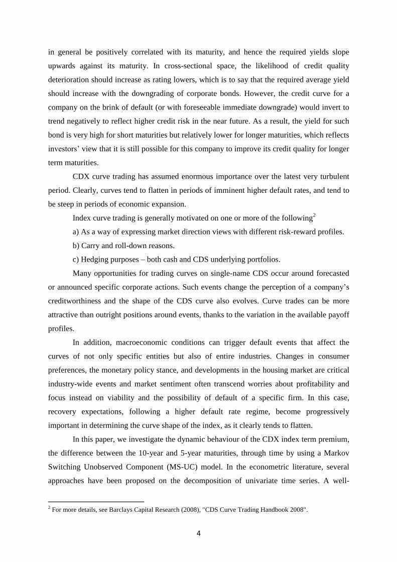
The remaining subsections present our stylized model of analysis. We first show how
to construct the two components that drive the evolution of the CDX term premium. We
outline next the state space representation of the system and our extension of modeling
Markov switching disturbance terms.
2.1 Stationary and Random Walk Components in State Space Representation
Let 1,tX represents the stationary component that drives the term premium, and
assume that 1,tX is an Ornstein-Uhlenbeck process, whose dynamic evolution can be
described by the stochastic differential equation
1, 1, 1 1,t t tdX k X dt dZ
EQUATION 1
where is the target equilibrium or mean value supported by fundamentals; 1 0 is
the scale of volatility that the exogenous shocks can transmit to the dynamics of 1,tX ;
1,tdZ is
the standard Brownian motion with zero mean and unity variance that generate random
exogenous shocks; 0k is the rate by which these shocks dissipate and the variable, 1,tX ,
reverts back to its mean. The Ornstein-Uhlenbeck process is an example of a Gaussian
process that admits a stationary probability distribution and has a bounded variance. In
contrast to the Brownian motion process that has constant drift term, the former allows for a
drift term that is dependent on the current value of the process. If the current value of the
process is lower than its long-term mean value, the drift term will be positive in order to bring
the process back to its long-term mean value. If, on the other hand, the current value of the
process is greater than its long-term mean value, the drift term will be negative in order to
drag down the process back to its long-term mean value. In other words, this is a mean-
reverting process. Setting 1, 1,, kt
t tf X t X e and applying the Ito’s Lemma to this function,
this leads to
1, 1 1,, kt kt
t tdf X t k e dt e dZ
EQUATION 2
Integrating both sides of Equation 2, we obtain

12
1, 1,0 1 1,
01
t k t skt kt
t sX X e e e dZ , 0 s t
EQUATION 3
where
1,0X is the initial value of the process and the first and the second moments are
given by
1, 1,0
2 2
1
1,
1
1
2
kt kt
t
kt
t
E X X e e
eVar X
k
EQUATION 4
The Ornstein-Uhlenbeck process is one of several widely used approaches to model
stochastically interest rates, exchanges rates and stock prices. The advantages of its simple
and tractable solutions, under continuous-time framework, have been embodied in many
empirical asset pricing models. The econometric modeling, however, emphasizes the
discrete-time representation of stochastic processes. Consequently, the exact discrete time
model corresponding to Equation 1 is given by the following AR(1) process
1, 1, 1 1,1 k t k t
t t tX e e X Z
EQUATION 5
where 1250
t is the sampling interval and
1 1
1
2
k te
k
. From this
expression, it is immediately clear that 0k implies 1k te and hence stationarity, 0k
or 0t implies 1k te and the model converges to a unit root model.
Now, let 2,tX be the second component that drives the term premium. We assume that
it follows a driftless RW process as shown in Equation 6
2, 2 2,t tdX dZ
EQUATION 6
where 2 is the scaled volatility parameter and 2,tdZ is the standard Brownian motion
that can be assumed to be either dependent or independent of 1,tdZ .The discrete time version
of Equation 6 yields

13
2, 2, 1 2 2,t t tX X Z
EQUATION 7
The RW process has long been a popular choice for modeling the price dynamics of
financial assets. In continuous time financial models, the price of stocks and stock indices are
modeled as geometric Brownian motions. It is relatively straightforward to show that the
geometric Brownian motion of the price dynamic is equivalent to a RW path followed by the
logarithm of the price in discrete time. The efficient market hypothesis in fact states that a
financial asset’s price follows a RW process, which literally assumes that the asset’s price at
time t is determined by its previous time period price and the instantaneous impact of the
new flow of information. Although a RW process, like the one described in Equation 7, has
infinite unconditional mean and variance, the conditional mean and variance can be measured
as
2, 2, 1
2
2, 2
t t t
t t
E X X
Var X
EQUATION 8
where the conditional expectation of the process at current time t depends only on the
observation at previous time period.
Given the two unobserved components, constructed using Equation 1 to Equation 7,
we estimate the parameter space , as given by the system in Equation 9, with the dynamics of
the two components in a Bayesian updating manner, namely the Kalman filter algorithm
based on a state space system. State space representation is usually applied on dynamic time
series models that involve unobserved variables (see, e.g., Engle and Watson (1981),
Hamilton (1994), Kim and Nelson (1989)). In our modeling, the fact that the two driving
forces of the CDX index term premium - stationary and RW components - are assumed to be
unobserved state variables leads to the justification of using the state space representation. A
typical state space model consists of two equations. One is a state equation that describes the
dynamics of unobserved variables, which is shown below in Equation 9; and the other one is
the measurement equation that describes the relation between measured variables and the
unobserved state variables, as shown in Equation 10.
14
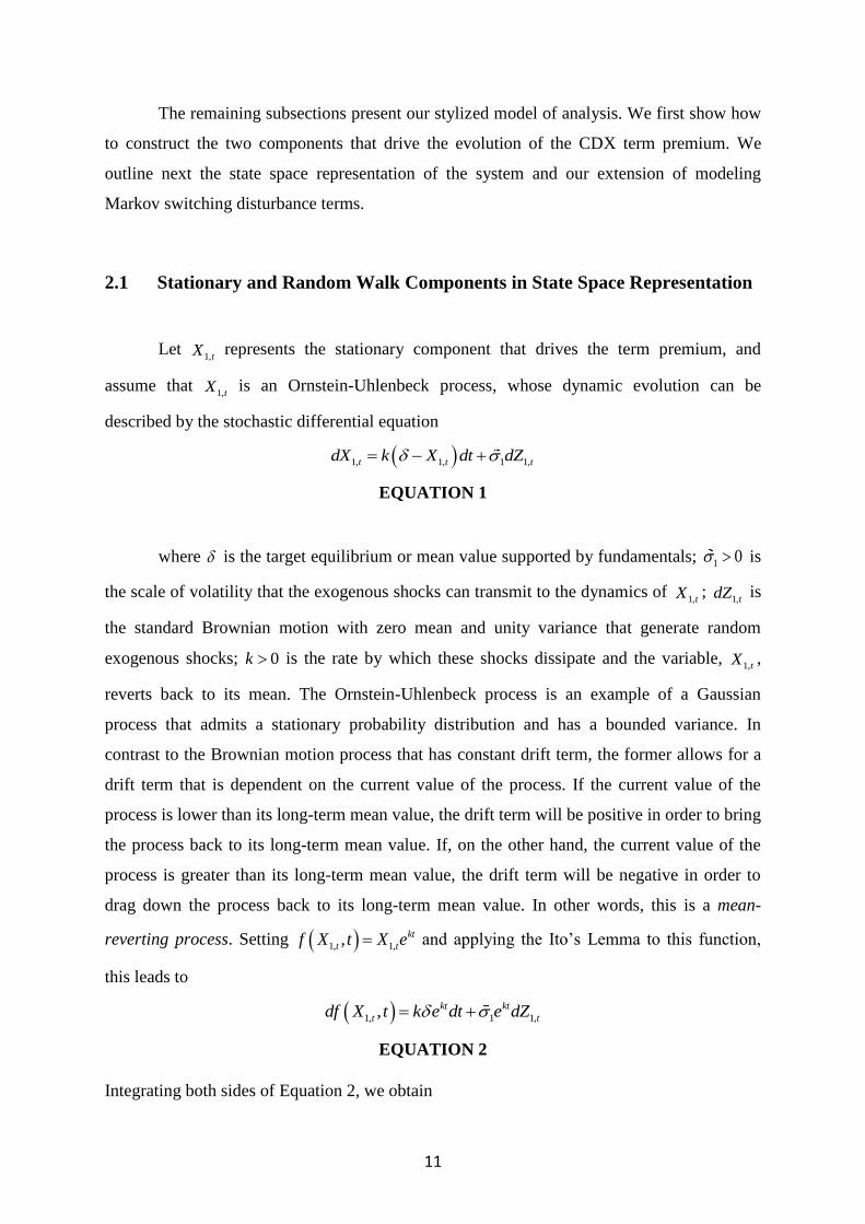
1, 1, 1 1,
2, 2, 1 2,
21, 1 1 2 12
22, 2 1 21 2
1 0,
0 10
0~ ,
0
k t k tt t t
t t t
t
t
X Xe e
X X
t
EQUATION 9
1, 2,t t tY X X
EQUATION 10
In Equation 9, the covariance terms 1 2 12 and 2 1 21 will be zero under the
assumption of independence between the two disturbance terms (the correlation between the
two disturbance terms - 12 - is zero).
In compact form, Equation 9 can be rewritten as
1 ,
~ 0,
t t t
t
X C FX
Q
EQUATION 11
where1,
2,
t
t
t
XX
X
, 1
0
k teC
,0
0 1
k teF
, 1,
2,
t
t
t
and
2
1 1 2 12
2
2 1 21 2
Q t
.
The measurement equation, as described by Equation 10, links linearly the term
premium of the CDX index to the stationary and RW components. Rewriting this expression
in a compact form, Equation 10 reduces further to yield
t tY HX
EQUATION 12
where tY is the term premium series and 1 1H represents the weights of the two
components in the term premium.

15
2.2 State Space Model with Markov Switching Disturbances
An additional feature of our model is to allow each component’s disturbance term to
depend on different states of the economy. In practice, we let the volatilities of the
disturbance terms to switch between high and low volatility regimes. Formally, we assume
that 2
1 and 2
2 in Equation 9 are driven by two discrete-valued, independent unobserved
first-order Markov chain processes 1, 0,1tS and 2, 0,1tS given by
2 2 2 2 2
1 1, 1 1, 1 1 1
2 2 2 2 2
2 2, 2 2, 2 2 2
1 ,
1 ,
t H t L H L
t H t L H L
S S
S S
EQUATION 13
When both
1,tS and 2,tS are zeros, the two components will be in the high volatility
state as 2 2
1 1H and 2 2
2 2H ; similarly if both 1,tS and
2,tS equal 1, the two components will
be in the low volatility state since 2 2
1 1L and 2 2
2 2L . The two remaining scenarios then
categorize situations where the first component is in the high volatility state while the second
is in the low (1, 2,0, 1t tS S ) and where the first component is in the low volatility state while
the second is in the high (1, 2,1, 0t tS S ). This is a Markovian chain process which means that
the current value of the process at time t depends only on its previous value at time 1t . The
likelihood for the process to remain at the previous value or change to the alternative depends
on the transition probabilities from one state to the other, which are shown below as
1,00 1, 1, 1
1,11 1, 1, 1
2,00 2, 2, 1
2,11 2, 2, 1
Pr 0 | 0
Pr 1| 1
Pr 0 | 0
Pr 1| 1
t t
t t
t t
t t
p S S
p S S
p S S
p S S
EQUATION 14
Equivalently, the two transition probability matrices for each disturbance term can be
written as
1,00 1,01 2,00 2,01
1 2
1,10 1,11 2,10 2,11
, p p p p
p pp p p p
EQUATION 15

16
where , , , 1Pr |q ij q t q tp S j S i
with 2
1
1 , ij
j
p i
and 1,2q .
The estimation of the transition probabilities as shown above requires the choice of
the appropriate functional forms of the probability functions that govern the Markov chain
variables. Since the transition probabilities have to be bounded within 0,1, the usual choice
is the adoption of the logistic transformation on the probability terms that are given by
1,0
1,00 1, 1, 1
1,0
1,01 1,00
1,1
1,11 1, 1, 1
1,1
1,10 1,11
2,0
2,00 2, 2, 1
2,0
2,01 2,00
2,11 2, 2, 1
expPr 0 | 0
1 exp
1
expPr 1| 1
1 exp
1
expPr 0 | 0
1 exp
1
ePr 1| 1
t t
t t
t t
t t
dp S S
d
p p
dp S S
d
p p
dp S S
d
p p
p S S
2,1
2,1
2,10 2,11
xp
1 exp
1
d
d
p p
EQUATION 16
where
1,0d ,1,1d ,
2,0d and 2,1d are the unconstrained parameters. Appendix A contains a
detailed account of the estimation procedures used in this model.
3. Data
In this section, we describe the relevant CDs and the data series used in the study.
CDS contracts are by nature over-the-counter. As a result, the availability and quality
of the data are not as dependable as those of exchange-based transactions. CDS data are
mainly collected by large investment banks which only record their own entering
transactions. Although professional data vendors are the primary source of CDS research
data, the data suffer the following pitfalls: (1) as in Zhu (2004), data prior to 1999 are very
limited; (2) the frequency of CDS transaction data is low, therefore, the usual instantaneous
lead-lag analysis which use much higher frequency data may not be robust; (3) CDS prices

17
are usually obtained as “quoted” prices which may not reflect the actual information
contained in trading prices; (4) CDS data are truncated in the way that the majority contracts
have a maturity of 5 years with nominal amount of $5 million or $10 million; (5) CDS data
are usually unevenly spaced with many spurious observations in time series4.
To circumvent the above mentioned limitations, we restrict our sample of analysis to
the CDS tranche index market, specifically to the North American CDX investment-grade
indices. In these indices, all 125 single-name credits have equal weights in the portfolio. The
Dow Jones CDX IG five-year index is a basket of CDSs on 125 names for the U.S.
investment-grade market. Each reference entity has a weight of 0.8%. We use a
representative dataset of daily CDS prices for the North American CDX tranche index and
focus our analysis on the most liquid segments of the CDX index market, which are the 5-
year and 10-year maturities. The analysis is based on daily data spanning from 2004 to 2009.
The main source of CDX data is Markit.
In our sample period (August, 5. 2004 to July, 23. 2009), as shown in Table 2 and
Figure 1, the average premium is 87.3161 basis points for the CDX 5-year index and 95.9463
for the CDX 10-year index. The CDX 5-year index reaches its maximum spread (283 basis
points) on September, 16 2008, which is the day after the announcement of Lehman Brothers
default. Similarly, the CDX 10-year index reaches its maximum premium (251 basis points)
on the same day, as it is reflected in the negative slope of the credit curve. Not only the
volatility of the CDS indices increased dramatically as of July 2007, but also the levels of
these indices started to rise significantly at the onset of the crisis. The unprecedented
financial turmoil directly raised investors’ expectations on imminent defaults of firms’ debts,
especially of those financial firms heavily exposed to sub-prime-mortgage lending. From the
second panel of Figure 1, we can see that the term premium of the CDX 10-year – 5-year
index becomes negative at the start of 2008, suggesting an increase of investors’ concerns
over short-term default risk. Nevertheless, market sentiment remains unchanged over long-
term horizons.
Daily Federal Fund Rates (FFR) are obtained from the St. Louis FRED database.
Daily slope of the yield curve (SLOPE101), calculated using 10-year and 1-year U.S.
Treasury bond yields, are from Thomson Reuters© Datastream. S&P 500 index daily
observations are obtained from Thomson Reuters© Datastream. VIX index data are from the
Chicago Options Mercantile Exchange (CBOE). The descriptive statistics of monetary policy
4 An in-depth discussion of CDS data quality can be found in: Blanco, Brennan and Marsh (2005).

18
and equity market condition variables are also presented in Table 2 and Figure 2 depicts their
evolution over the sample period.
TABLE 2: DESCRIPTIVE STATISTICS OF THE DATA SERIES
CDX5 CDX10
Term
Premium FFR SLOPE101 SP500RTN VIX
Mean 87.3161 95.9463 8.6302 3.289400 1.268461 -0.0001 21.2356
Median 53.0000 77.0000 22.0000 3.620000 1.045000 0.0007 15.6300
Maximum 283.3708 251.3626 33.0000 5.410000 4.010000 0.1042 80.8600
Minimum 29.0000 54.0000 -53.3332 0.080000 -0.780000 -0.0947 9.8900
Std. Dev. 62.6127 41.3712 22.3793 1.810837 1.232534 0.0156 12.8773
Skewness 1.1973 1.1911 -1.3317 -0.491720 0.277599 -0.2528 1.8976
Kurtosis 3.2020 3.4167 3.6070 1.884992 1.911517 12.3573 6.5427
Jarque-Bera 281.2800 284.8754 363.4610 105.9148 71.54148 4277.3390 1312.9130
Probability 0.0000 0.0000 0.0000 0.000000 0.000000 0.0000 0.0000
Observations 1169 1169 1169 1169 1169 1169 1169
10/09/04 29/03/05 15/10/05 03/05/06 19/11/06 07/06/07 24/12/07 11/07/08 27/01/09
50
100
150
200
250
10/09/04 29/03/05 15/10/05 03/05/06 19/11/06 07/06/07 24/12/07 11/07/08 27/01/09
-40
-20
0
20
CDX 5 Year
CDX 10 Year
Term Premium
FIGURE 1: CDX-5 YEAR, CDX-10 YEAR AND CDX TERM PREMIUM

19
0
1
2
3
4
5
6
250 500 750 1000
FFR
-1
0
1
2
3
4
5
250 500 750 1000
SLOPE101
-.10
-.05
.00
.05
.10
.15
250 500 750 1000
SP500RTN
0
20
40
60
80
100
250 500 750 1000
VIX
FIGURE 2: ACTUAL PLOTS OF: FFR, SLOPE101, S&P 500 RETURNS AND VIX
INDEX
4. Empirical Results
Using the methodology described in section 2, we estimate a series of nested Markov-
switching unobserved component models, followed by a battery of tests on model
specification to determine the preferred model that will be used in the empirical analysis.
4.1 Model selection tests
It is well known that for Markov-switching models the standard likelihood ratio test
of the null hypothesis of linearity does not have the usual 2 distribution. The reason is that
there are nuisance parameters which cannot be identified under the null hypothesis. As a
result, the scores evaluated at the null hypothesis are identically zero. Hansen (1992) and
Garcia (1998) introduce alternative tests of the linearity against regime switching. In this
paper, we use Hansen (1992) procedure, which provides an upper bound of the valuep for

20
linearity, to determine the significance of improvement for allowing Markov-switching
disturbance terms in the two components. In addition, we also consider more conventional
ways of selecting models based on the Akaike Information Criterion (AIC) and Schwarz
Bayesian Information Criterion (BIC). Finally, we verify our model selection results by
running a series of residual diagnostic tests to see if the selected model could capture serial
correlation and heteroskedasticity in the data series.
To implement Hansen’s procedure (1992), we need to evaluate the constrained
likelihood under the null hypothesis over a grid of values for the nuisance parameters.
Defining the restricted model under the null hypothesis of no regime switching of the two
components' disturbance terms as represented in equations 9-10 with 12 21 0 , and the
alternative model under the assumption of Markov-switching disturbance terms as involving
equations 13-16, we have nuisance parameters 1 2 1,00 1,11 2,00 2,11, , , , ,H H p p p p . The grids
that we use for 1H and 2H are 1,2.5 and 5,10.5 , respectively, each in increment step of
0.5. The grids for 1,00 2,00,p p varies from 0.7 to 0.9 in increment step of 0.05 and for
1,11 2,11,p p from 0.8 to 0.9 in increment step of 0.05. The Hansen test applied as described
above, yields a conservative valuep of 0.001, which clearly indicates a strong rejection of
linearity in favoring of Markov-switching disturbance terms.
TABLE 3 and Table 4 contain the selection criteria results for models enabling
correlated disturbance terms and models which are zeros correlations restricted. While AIC
and BIC suggest that correlated models may perform better, likelihood ratio tests show that
Model 1 and Model 2 better fit the data than Model 5 and 6, respectively. However, note that
the improvement in likelihood value when allowing correlations and all parameters to switch
between regimes (Model 8) is remarkable. In Table 5 we also report the likelihood ratio tests
within each nested group and we can see that the most flexible model (Model 8) significantly
outperforms all the models. We verify this result with the residual diagnostic tests in Table 6,
where we test the overall randomness of the residuals of the models (summation of the
disturbance terms of the two components) with the null hypothesis of assuming randomness.
We report two Ljung-Box Q statistics for each model: one is the autocorrelation Q statistics
based on the standardized residuals up to 20 lags; the other one is the ARCH effect Q
statistics based on the squared standardized residuals up to 20 lags. From Table 6, the Q
statistics suggest Model 8 as the best performing model, since it captures both the
autocorrelation and ARCH effects in the residuals.

21
TABLE 3: MODEL SELECTION RESULTS
Model Specifications
Number of
parameters AIC BIC ln L
Model 0: 12 21 0 , 1 regime 4 3.1346 3.1521 -1798.3900
Model 1: 12 21 0 10 2.8000 2.8439 -1600.0100
Model 2: 12 21 0 , 2k 11 2.7772 2.8255 -1585.9164
Model 3: 12 21 0 , 2 11 2.7625 2.8108 -1577.4354
Model 4: 12 21 0 , 2k , 2 12 2.6900 2.7426 -1534.7273
Model 5: 12 21 0 14 2.8012 2.8627 -1596.6954
Model 6: 12 21 0 , 2k 15 2.7822 2.8480 -1584.7574
Model 7: 12 21 0 , 2 15 2.7622 2.8281 -1573.2809
Model 8: 12 21 0 , 2k , 2 16 2.6710 2.7412 -1519.8149
Note: Model 0 refers to system of equation 9-10 assuming 12 21 0 . Model 1 builds on
Model 0 with Markov-switching variances defined in equations 13-16; Model 2 builds on
Model 1 but allow k to switch regimes; Model 3 builds on Model 1 but allow to switch
regimes; Model 4 builds on Model 1 but allow both k and to switch regimes; Models 5-8
differ from 1-4 for allowing correlations between the two components' disturbance terms.
ln L denotes the natural logarithm of likelihood value. AIC denotes the Akaike Information
Criterion and BIC denotes the Schwarz Bayesian Information Criterion. A smaller statistic of
AIC or BIC corresponds to smaller estimated Kullback-Leibler distance from the true model.
TABLE 4: LIKELIHOOD RATIO TESTS ON CONSTRAINT 12 21 0
Constraint: 12 21 0 Likelihood ratio p-value
Model 1 to Model 5 6.6292 0.1568
Model 2 to Model 6 2.3180 0.6775
Model 3 to Model 7 8.3089 0.0809
Model 4 to Model 8 29.8248 5.31336E-06
TABLE 5: LIKELIHOOD RATIO TESTS WITHIN GROUPS
Constraints Likelihood ratio p-value
Group of models apply 12 21 0
Model 1 to Model 2: 2 0k 28.1871412 0.0000
Model 1 to Model 3: 2 0 45.1492514 1.82575E-11
Model 1 to Model 4: 2 2 0k 130.565418 4.44713E-29
Group of models apply 12 21 0
Model 5 to Model 6: 2 0k 23.8759758 1.02746E-06
Model 5 to Model 7: 2 0 46.8289503 7.74606E-12

22
Model 5 to Model 8: 2 2 0k 153.761032 4.08523E-34
TABLE 6: RESIDUAL DIAGNOSTIC TESTS
Autocorrelation ARCH Autocorrelation ARCH
Lags Q-stats p-value Q-stats p-value Q-stats p-value Q-stats p-value
Model 0
1 3.3651 0.0666 55.4375 1.00E-13
5 6.4061 0.2687 56.5142 6.37E-11
10 21.4859 0.0179 84.9913 5.00E-14
20 51.2066 0.0001 128.0163 0.00E+00
Model 1 Model 5
1 5.8659 0.0154 12.4945 0.0004 0.002 0.9643 1.4605 0.2268
5 38.7978 0 77.4846 0 21.916 0.0005 12.6867 0.0265
10 46.7586 0 98.3647 0 39.9475 0 21.0755 0.0206
20 127.264 0 157.386 0 91.3123 0 42.9094 0.0021
Model 2 Model 6
1 10.665 0.0011 2.0368 0.1535 12.7731 3.52E-04 2.2811 0.131
5 64.4022 0 6.0608 0.3003 69.3635 0.00E+00 5.6359 0.3433
10 129.4365 0 38.6211 0 140.9098 0.00E+00 48.6666 0
20 244.9473 0 59.528 0 256.8626 0.00E+00 67.5147 0
Model 3 Model 7
1 34.5333 4.19E-09 0.3524 0.5528 14.6746 1.28E-04 0.0017 0.9673
5 73.5529 0.00E+00 13.7145 0.0175 22.747 3.77E-04 0.0029 1
10 94.9219 0.00E+00 37.0741 0.0001 50.5479 2.00E-07 1.4622 0.999
20 114.7697 0.00E+00 97.5292 0 76.9609 0.00E+00 1.4862 1
Model 4 Model 8
1 9.6918 0.0019 0.0337 0.8544 1.0875 0.297 0.0044 0.9468
5 19.6283 0.0015 1.3234 0.9325 4.0601 0.5408 0.0107 1
10 37.2164 0.0001 13.1973 0.2128 9.7284 0.4646 0.0267 1
20 56.5368 0 16.2277 0.7024 22.5042 0.3138 0.1733 1

23
4.2 Estimates of the Markov-switching unobserved component model
Table 7 reports the maximum likelihood estimates of Model 8, the most flexible and
best performing model suggested by the model selection procedures considered above. The
first noticeable result is the two regime dependent long term equilibriums of the stationary
component: 8.4516 as in the low volatility regime and -0.5633 in the high regime. As can be
seen, during the calm period (from 05 August 2004 to 31 December 2007), the slope along
the credit curve is positive since the term premium is the compensation for default risk in 5
years’ time. However, since the outbreak of the crisis (August 2007), severe strains in
financial markets, banks' assets writedowns and diminishing liquidity in funding markets
raised the level of uncertainty about corporate default risk. The inversion of the credit curve,
as embedded in a negative CDX index term premium, vividly capture this deteriorating
outlook.
TABLE 7: ESTIMATION RESULTS OF MODEL 8
Parameters Estimate Std. Error
L 8.451611479 0.19272889
H -0.56331625 0.22729646
Lk 465.0780475 30.5714495
Hk 23.94429862 3.79151988
1,L 0.006555485 0.01754211
1,H 7.238340818 0.74796998
2,L 0.000709143 0.00671695
2,H 4.115509141 0.23609131
1 ,2L L 0.882338837 2.69775828
1 ,2H L -0.8868773 23.1607869
1 ,2L H -0.62831343 4.08740951
1 ,2H H -0.72940729 0.21734431
1,LLp 0.995606738 0.00148892
1,HHp 0.999997253 1.68E-06
2,LLp 0.964267884 0.00110252
2,HHp 0.97346475 0.00067856
ln L -1519.81491

24
Note: Subscript L denotes Low volatility regime and H denotes High volatility regime.
Subscript T denotes Stationary component and R denotes Random walk component.
The second remarkable result is the regime dependent mean reverting speed for the
stationary component. During non-crisis periods, asset prices are less likely to stay high or
low period-to-period but mean revert quickly to their long-term equilibrium values. In other
words, mean reverting assets prices imply a low probability of ending up in the tail of the
distribution. Our estimation of the measure of mean reverting speed ( k ) is 465.07 in a low
volatility regime, which translates to a first-order autocorrelation of 0.1556. The speed in the
high volatility regime, on the other hand, falls to 23.94 or 0.9087 in terms of first-order
autocorrelation, which suggests a very persistent behavior of the stationary component in the
high volatility regime.
Next, we look at the volatilities of the stationary and RW components in each regime.
In terms of stationary shocks, the estimated volatility in the low volatility regime is positive
but statistically insignificant. This is primarily due to the very high mean reverting speed in
the low volatility regime. Therefore, the variations in the low volatility regime are barely
zero. It is more clearly shown in Figure 3 that the stationary component's variation in low
volatility regime is tight at around 8.45 and the largest change is only 1.4 basis points. On the
other hand, the scale of the variation for the stationary component in the high volatility
regime is by far higher than in the non-crisis period, with an estimated annual volatility of
7.238.
The distinguishing feature of our model is that it allows us to decompose the term
premium into two correlated driving components. The filtered RW and the stationary
components with the associated probabilities of switching regimes are displayed in Figure 4
and Figure 5. In the first part of the sample period, temporary volatile movements in the RW
and stationary components are induced by severe shocks such as the GM and Ford
downgrade events of May 2005. In the subsequent period, the credit market enjoyed a rapid
growth in terms of both trading volumes and products innovation. During this time period,
both components stay in the low volatility regime, as reflected by a flat CDX credit curve.
The frequent regime changes of the RW component start taking place in the aftermath of
Countrywide’s bankruptcy. In fact, on August, 15 2007, Countrywide Financial, the largest
mortgage lender in the United States, announced that the foreclosure and mortgage
delinquencies had risen to their highest level since early 2002. Since then, because of that
episode and of the events around the onset of the subprime mortgage crisis, the CDX index

25
term premium exhibits a downward trend. Ironically, that event occurred just one month after
the DJIA index hit its historical record level of 14,000 (on July, 19 2007).

26
FIGURE 3: SNAPSHOT OF THE STATIONARY COMPONENT IN THE LOW VOLATILITY REGIME

27
FIGURE 4: STATIONARY COMPONENT AND ITS PROBABILITIES TO SWITCH TO THE HIGH VOLATILITY REGIME

28
FIGURE 5: RANDOM WALK COMPONENT AND ITS PROBABILITIES TO SWITCH TO THE HIGH VOLATILITY REGIME

29
On the other hand, as shown in Figure 4, the stationary component enters a high
volatility period from the beginning of 2008. Increased credit-related writedowns for
individual banks (e.g. Citigroup) owe to a further deterioration in the corporate debt and
prime residential mortgage markets, as the crisis originally centered in subprime mortgages
spilled over to adversely affect economic prospects more broadly. On January, 22 2008, the
Federal Reserve cut the Fed funds target rate to 3.5% - an unprecedented decision, taken
between scheduled meetings, and the largest single cut in 23 years. The move followed the
biggest one day loss on world stock exchanges in almost six years. The rate is reduced further
to 3% on January, 30 2008. On March, 14 2008, Bear Sterns' demise brought about a
dramatic increase in stock market volatility and liquidity shortages in funding markets. As
illustrated in Figure 4, the resulting decline of the stationary component on that day captures
investor confidence-induced downward spirals. The subsequent abrupt jumps occur on July,
13 2008 and November, 23 2008 when the US authorities announced the nationalization of
Fannie Mae and Freddie Mac and a rescue package of Citigroup.
Although the probability of the stationary component to switch to the high volatility
regime accurately signal greater market volatility since early 2008, it is quite evident from
inspection of this data that the probability for the RW component to switch into the high
volatility regime is close to zero at the occurrence of extreme credit events, such as the Bear
Stearn’s and Lehman Brothers’ default announcements. At first sight, this counter-intuitive
result may be difficult to understand. It conveys the message that credit market uncertainties,
as measured by the conditional variance of the term premium, decline significantly with the
abrupt unveiling of tail risk events.

30

31
FIGURE 6: CONDITIONAL VARIANCE OF THE TERM PREMIUM WITH EACH COMPONENTS' PROBABILITIES TO
SWITCHING TO THE HIGH VOLATILITY REGIME

32
Figure 6 plots the conditional variance derived from model 8. Using the definition of
Kalman filter provided in the previous section, the conditional forecast error variance is given
by
1, 1 1, 2, 1 2, 1, 1 1, 2, 1 2,
| 1 | 1 't t t t t t t tS S S S S S S S
t t t tf HP H
EQUATION 17
which can be regarded as the implied conditional variance of the CDX term premium.
Since this conditional variance depends on the two Markov chain processes, combining the
filtered probabilities of states 1, 1 1, 2, 1 2,
1 1 1 1
1, 1 1, 2, 1 2, 1
0 0 0 0
Pr , , , |t t t t
t t t t t
S S S S
S i S j S i S j I
with Equation 17, we can calculate the conditional variance as a product of these two
equations, based on the available information at time 1t . From Figure 6 we can observe that
the conditional variance, in the immediate aftermath of Bear Stern’s bailout (March, 14
2008), remains at low levels for a few days. What is particularly striking is that the
probability for the RW component to switch into the high volatility regime falls back to a
near-zero value at the outbreak of the crisis. In the sub-sample period surrounding Lehman
Brothers’ default, the conditional variance of the CDX term premium is much bigger than in
the Bear Stern’s bailout period. Consequently, the probability of the RW component to
switch into the high volatility regime initially falls back to a near-zero value, but rebounds
very rapidly in the subsequent days as investors begin to worry about the stability of other
systemically important financial institutions. Our results show that the persistent co-
movement between the high conditional variance of the CDX term premium and the
probability of the RW component switching into the high volatility regime disappears during
the financial crisis period. This suggests that the RW and the stationary components may
behave differently depending on whether the financial system is experiencing a systemic
crisis or not.
4.3 VAR Analysis
We now test for the impact of observed economic and financial variables on the
unobserved stationary and RW components, in the context of the following VAR (4) model5
5 The order of the VAR is established using the SBC criterion.
33
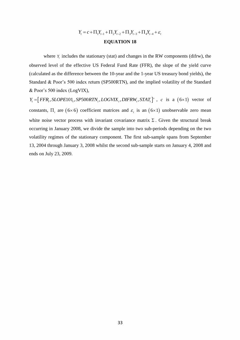
1 1 2 2 3 3 4 4t t t t t tY c Y Y Y Y
EQUATION 18
where
tY includes the stationary (stat) and changes in the RW components (difrw), the
observed level of the effective US Federal Fund Rate (FFR), the slope of the yield curve
(calculated as the difference between the 10-year and the 1-year US treasury bond yields), the
Standard & Poor’s 500 index return (SP500RTN), and the implied volatility of the Standard
& Poor’s 500 index (LogVIX),
, 101 , 500 , , , 't t t t t t tY FFR SLOPE SP RTN LOGVIX DIFRW STAT , c is a 6 1 vector of
constants, i are 6 6 coefficient matrices and t is an 6 1 unobservable zero mean
white noise vector process with invariant covariance matrix . Given the structural break
occurring in January 2008, we divide the sample into two sub-periods depending on the two
volatility regimes of the stationary component. The first sub-sample spans from September
13, 2004 through January 3, 2008 whilst the second sub-sample starts on January 4, 2008 and
ends on July 23, 2009.

34
-0.25
0.00
0.25
0.50
0.75
1.00
1 2 3 4 5 6 7 8 9 10
Accumulated Response of DIFRW to FFR
-0.25
0.00
0.25
0.50
0.75
1.00
1 2 3 4 5 6 7 8 9 10
Accumulated Response of DIFRW to SLOPE101
-0.25
0.00
0.25
0.50
0.75
1.00
1 2 3 4 5 6 7 8 9 10
Accumulated Response of DIFRW to SP500RTN
-0.25
0.00
0.25
0.50
0.75
1.00
1 2 3 4 5 6 7 8 9 10
Accumulated Response of DIFRW to LOGVIX
-0.25
0.00
0.25
0.50
0.75
1.00
1 2 3 4 5 6 7 8 9 10
Accumulated Response of DIFRW to DIFRW
-0.25
0.00
0.25
0.50
0.75
1.00
1 2 3 4 5 6 7 8 9 10
Accumulated Response of DIFRW to STAT
-.04
-.02
.00
.02
.04
.06
.08
1 2 3 4 5 6 7 8 9 10
Accumulated Response of STAT to FFR
-.04
-.02
.00
.02
.04
.06
.08
1 2 3 4 5 6 7 8 9 10
Accumulated Response of STAT to SLOPE101
-.04
-.02
.00
.02
.04
.06
.08
1 2 3 4 5 6 7 8 9 10
Accumulated Response of STAT to SP500RTN
-.04
-.02
.00
.02
.04
.06
.08
1 2 3 4 5 6 7 8 9 10
Accumulated Response of STAT to LOGVIX
-.04
-.02
.00
.02
.04
.06
.08
1 2 3 4 5 6 7 8 9 10
Accumulated Response of STAT to DIFRW
-.04
-.02
.00
.02
.04
.06
.08
1 2 3 4 5 6 7 8 9 10
Accumulated Response of STAT to STAT
Accumulated Response to General ized One S.D. Innovations ± 2 S.E.
FIGURE 7: ACCUMULATIVE GERNERALIZED IMPULSE RESPONSE FUNCTIONS OF THE VAR MODEL IN THE PRE-
FINANCIAL CRISIS PERIOD (013/09/04 TO 03/01/08)

35
-1
0
1
2
1 2 3 4 5 6 7 8 9 10
Accumulated Response of DIFRW to FFR
-1
0
1
2
1 2 3 4 5 6 7 8 9 10
Accumulated Response of DIFRW to SLOPE101
-1
0
1
2
1 2 3 4 5 6 7 8 9 10
Accumulated Response of DIFRW to SP500RTN
-1
0
1
2
1 2 3 4 5 6 7 8 9 10
Accumulated Response of DIFRW to LOGVIX
-1
0
1
2
1 2 3 4 5 6 7 8 9 10
Accumulated Response of DIFRW to DIFRW
-1
0
1
2
1 2 3 4 5 6 7 8 9 10
Accumulated Response of DIFRW to STAT
-4
-2
0
2
4
6
1 2 3 4 5 6 7 8 9 10
Accumulated Response of STAT to FFR
-4
-2
0
2
4
6
1 2 3 4 5 6 7 8 9 10
Accumulated Response of STAT to SLOPE101
-4
-2
0
2
4
6
1 2 3 4 5 6 7 8 9 10
Accumulated Response of STAT to SP500RTN
-4
-2
0
2
4
6
1 2 3 4 5 6 7 8 9 10
Accumulated Response of STAT to LOGVIX
-4
-2
0
2
4
6
1 2 3 4 5 6 7 8 9 10
Accumulated Response of STAT to DIFRW
-4
-2
0
2
4
6
1 2 3 4 5 6 7 8 9 10
Accumulated Response of STAT to STAT
Accumulated Response to General ized One S.D. Innovations ± 2 S.E.
FIGURE 8: ACCUMULATIVE GENERALIZED IMPULSE RESPONSE FUNCTIONS OF THE VAR MODEL IN THE POST-
FINANCIAL CRISIS PERIOD (04/01/08 TO 23/07/09)

36
To evaluate the relationships between the two components and monetary policy and
stock market variables, we compute the accumulated generalized impulse response functions,
which trace out the responsiveness of the dependent variables to one unit generalized shock
to each of the variables in the VAR system. These impulse response functions provide useful
insights into the dynamic properties of the system.
As forecasting variables of the variation in the term premium of the CDX index, these
monetary policy and stock market variables appear to impact differently on the two
components, before and after the onset of the crisis. Figure 7 shows the accumulated
generalized impulse response functions of the VAR model in the pre-crisis period. The
responses of DIFRW and STAT to FFR are significantly positive, which is consistent with
the findings of Longstaff and Schwartz (1995) who document that corporate yield spreads
vary inversely with the benchmark short-term treasury yield. Since an increase in the
monetary policy rate would translate into an increase in the level of interest rate in normal
periods, a higher interest rate level will decrease the present value of future cash flows and
hence the value of default protection. This would lead to a tightening of the credit spread. If
the tightening of the spread is more severe for the shorter CDS maturities, the term premium
in the credit curve would increase as represented by a rise in the slope of the credit curve.
This result, as illustrated in Figure 7, is consistent with Longstaff and Schwartz (1995) who
suggests that the relationship between the CDX index spread and the risk-free interest rate
depends on the time horizon. Compared to the negative responses of DIFRW and STAT in
Figure 8, an increase in the monetary policy rate in the crisis-period would sharply reduce
liquidity, increasing the probability of imminent default. The obvious effect would be
widening the 5-year CDX premia and flattening the term premium of the CDX index.
The responses of the two components to SLOPE101 are negative but insignificant
during the pre-crisis period. Bedendo et al. (2007) report a negative relationship between the
slope of the US treasury yield curve and credit spreads. The reason is that when a positively
sloped yield curve is the outcome of an expansionary monetary policy, which will increase
future firm value and reduce default risk, the term premium decreases due to a decline in the
10-year premia. At the same time a steeper yield curve in normal time periods may indicate
an increase in the future short rate through the expectations channel. If the inflation risk
premium on longer term interest rates is very low (or even negative, see Kim and Wright
(2005)), the latter would change little in response to a continuous rise in short term rates
(Smith and Taylor (2009)). This effect, known as the “conundrum”, may make the shorter
maturity default protection contract more costly than those with longer maturities, and hence

37
increasing the 5-year credit risk premia. This will, in turn, reduce the term premium of the
CDX index. In contrast, during the crisis time period, any increase in the slope of the yield
curve caused by a reduction in the short rate would be regarded as a signal of liquidity
injections provided by central banks to contain systemic risks. Default protection premia (5-
year) will fall and this would subsequently lead to an increase in the term premium. The
positive responses of both DIFRW and STAT to an increase in the slope of the yield curve in
crisis period (Figure 8) lend support to this hypothesis.
In the pre-crisis period the initial responses to equity market returns and the implied
volatility index, have the opposite signs on DIFRW and STAT at the outset. Yet, at longer
lags, both components exhibit a positive (negative) relationship with the equity returns
(equity volatility). During the post-crisis period this initial divergence dissipates and both
factors strongly respond positively to equity returns and negatively to the VIX. Such finding
is consistent with the evidence in Bystrom (2006) who reports that on-the-run single-name
CDS spread is significantly negatively related to the equity returns for the period 2004-2006.
Scheicher (2006) also demonstrates that there is a significant contemporaneous link between
the CDS market and the stock market. The inverse relationship between the two components
and equity return volatility is broadly consistent with previous econometric evidence, as
illustrated by Campbell and Taksler (2003), Alexander and Kaeck (2008) and Zhang et al.
(2008). In the theoretical framework of Merton (1974), higher equity volatility means higher
probability of hitting the default barrier, which induces a higher compensation on holding the
bond in the form of larger credit spread. Although the positive (negative) responses to equity
return (equity return volatility) hold both in non-crisis and crisis periods, the magnitude of
responses in crisis period is far more pronounced.
To quantify the impact of all the observed variables on the unobserved factor we
compute the generalized variance decomposition over the two periods. The results are
presented in Tables 8 and 9. The key finding is the presence of strong effects attributable to
stock market variables on both components before and after the crisis. Initially, in the pre-
crisis period the impact of all the variables on both components is modest (Table 8). Stock
market returns and their volatility appear to be the variables exerting some influence on
DIFRW and STAT. Collectively they account for 7.5% of the DIFRW variability’s and
3.51% of the STAT’s variance.
In the post-crisis period of our sample (Table 9), approximately 13.5% of the
variation in the DIFRW can be attributed to a combination of stock market variables, the
monetary policy stance and the slope of the yield curve. More specifically, a substantial part

38
of this variation is primarily explained by the stock market variables (7.68%). For the
stationary component the same information set explains 16.44% of the variance, that is a
nearly fivefold increase compared to the previous period. The impact of monetary policy
alone is 4.2% compared to a previous value of 0.5%.
Importantly, our results indicate that during the crisis period, information pertinent to
the immediate valuation of firm’s assets, such as the stock market benchmark index and
monetary policy exerted relatively strong influence on the CDX term premium, compared to
factors such as the VIX and the slope of the yield curve.
Within the confines of the model, the crisis period is indicative of a significant change
to the fundamentals that determine the term premium, as captured by the stationary
component. The evidence from the RW component is indicative of increased volatility that
can be only partly explained by the set of the observed macro and financial variables included
in our analysis. In summary, these results do provide evidence that the inversion of the term
premium since the onset of the crisis is primarily attributable to the evolution of the stock
market and monetary policy. In particular, the drastic and immediate response of the Fed
played an important role in avoiding dramatic increases in the short (5-year) premia and
therefore helped stabilizing the short-term segment of the CDS market.
TABLE 8: GENERALISED VARIANCE DECOMPOSITION OF DIFRW AND STAT
IN THE PRE-FINANCIAL CRISIS PERIOD (SEPTEMBER 13, 2004 TO JANUARY
03, 2008)
Variance Decomposition of DIFRW:
Period S.E. FFR SLOPE101 SP500RTN LOGVIX DIFRW STAT
⁞
10 0.838 0.695 2.746 0.446 3.284 92.716 0.113
15 0.839 0.698 2.758 0.505 3.307 92.615 0.116
Variance Decomposition of STAT:
⁞
10 0.065 0.506 0.579 1.209 0.875 4.320 92.512
15 0.065 0.509 0.579 1.445 0.973 4.307 92.186

39
TABLE 9: GENERALISED VARIANCE DECOMPOSITION OF DIFRW AND STAT
IN THE POST-FINANCIAL CRISIS PERIOD (JANUARY 04, 2008 TO JULY 23,
2009)
Variance Decomposition of DIFRW:
Period S.E. FFR SLOPE101 SP500RTN LOGVIX DIFRW STAT
⁞
10 1.249 1.284 4.203 6.314 1.090 86.421 0.688
15 1.254 1.577 4.174 6.556 1.127 85.794 0.773
Variance Decomposition of STAT:
⁞
10 1.381 2.837 1.213 9.592 0.210 8.664 77.485
15 1.538 4.258 1.171 10.837 0.173 7.502 76.059
5. Conclusion
In this article, we estimate a Markov switching unobserved component model to
explain the evolution of the term premium of the most liquid CDS maturities for the North
American CDX index.
We consider an appropriately specified Markov Switching Unobserved Components
model as a reliable measure of volatility dynamics of the CDX index spread curve and
investigate the presence and significance of both monetary policy adjustments and stock
market returns for the US economy over the sample period September 2004 – July 2009.
To the best of our knowledge, this is the first direct empirically based evidence that is
brought on the evolution of the term premium of the CDS index market and its observed
macroeconomic and financial determinants.
To capture the magnitude of uncertainty in the CRT market, we decompose the level
of the CDX index term premium into two components. The first, the RW component is
assumed to capture the changes in volatility driving the term premium whereas the second, a
stationary AR(1) process, represents the fundamentals. Furthermore, we formulate a model
with time-varying regime-switching probabilities and regime dependent components.
Our results suggest that the inversion of the curve around September 2008 is largely
driven by abrupt moves in the stationary component, representing the evolution of the
fundamentals underpinning the probability of default in the economy. The component enters
the high volatility regime after a prolonged period of remarkable stability. Notably, by the
end of 2007, the stationary component exhibits slight turbulence in the low volatility regime,

40
but of a very different order of magnitude from the subsequent evolution of the component in
2008. The decline of the term premium accelerates sharply throughout the end of 2007 when
it partially reverses its trend. However, it remains in the high volatility regime in the final part
of the sample period. Interestingly, although the RW component appears to evolve in a very
stable and predictable manner from 2004 to 2008, it fluctuates somewhat intensively between
the low and high volatility regime over short periods of time during 2005 and towards the end
of 2007. From the beginning of the sub-prime crisis (August 2007) the component exhibits
downward movement but does not enter decisively the high volatility regime. Over the last
part of the sample, the component enters more frequently the low-volatility regime but in a
rather unpredictable manner, indicating that the uncertainty surrounding asset values still
remain elevated.
Remarkably, the inclusion of observed economic and financial variables to predict the
evolution of the unobserved components does a relatively good job only during the ‘crisis’
period. These variables are found to make a statistically significant contribution that is
consistent with economic theory. Indeed, we find robust evidence that the unprecedented
monetary policy response, of sharp rate reductions by the Fed during the crisis period, was
effective in reducing market uncertainty and helped to steepen the curve of the index thereby
mitigating systemic risk concerns. The impact of market volatility in flattening the curve and
exerting comparatively higher upward pressure on the 5-year CDX is substantially more
robust in the crisis period, as both components are significantly affected by the VIX measure.
It also appears that equity returns are important drivers of the term premium during both
periods. This impact results in a steepening of the curve as the current value of the underlying
‘collateral’ increases. Our results also suggest that in the pre-crisis period the RW component
associated with increased volatility displays a low reaction to the stock market. Additionally,
as expected the impact on the stationary component albeit positive is not significant. Yet,
from January 01, 2008 both components respond immediately and significantly to stock
market fluctuations. We demonstrate that the unprecedented stock market collapse is a very
important contributory factor to the inversion of the CDX index term premium.
Overall, this evidence implies that credit risk modeling that ignores this regime
dependent feature would bias the pricing of credit contracts. Developments in both the first
and second moments of the equity market have a lasting influence on both components, with
more pronounced effects during volatile market conditions.
The evolution of the CDX index in all maturities is an important signal of the ‘health’
of the economy over the short and long run. Sudden inversions indicate sharp deterioration of
41
the current economic conditions and increased probability of default. Such movements are
triggered by both the evolving stance of monetary policy and developments in the equity
markets that make a significant albeit modest contribution to their predictability.
This article is only a first step toward the development of a fully fledged consistent
framework to gain greater insight in the dynamics of the CDX curve indices across different
parts of the credit cycle and in the relationship between the shape of the term structure and
macro/financial variables fluctuations. Further research is warranted. Interesting possibilities
for further research include the consideration of an extended number of maturities and of
other index tranches, such the high-yield segment of the market. These extensions along with
a complementing examination of liquidity risks and the risk of spillovers will enhance our
understanding of the dynamics of such important markets, primarily from a systemic
viewpoint.

42
APPENDIX A
Estimation Procedure
To estimate the state space Markov switching model, described in detail in the
previous subsections, we use Kim’s filter (Kim (1994)), which is a numerical algorithm that
combine the Kalman filter in estimating state space models and the Hamilton filter in
estimating Markov switching models. In the conventional derivation of the Kalman filter for
an invariant parameter state space model, the goal is to make predictions of the unobserved
state variables based on the current information set, denoted | 1 1|t t t tX X I , where 1tI
represents all observed variables available at time 1t . The mean squared error of the
prediction, denoted as | 1t tP
, is | 1 | 1 | 1 1' |t t t t t t t t tP X X X X I . The Kalman filter
algorithm then implements a sequence of Bayesian updating on the unobserved variable tX
and the mean square error tP when observing a new data entry. The updated unobserved
variable|t tX , given the observation of the information set at time t , is formed as a weighted
average of | 1t tX
and new information contained in the prediction error, where the weight
assigned to this new information is called Kalman gain. This prediction and updating process
evolves over time and is conditional on the correctly estimated parameters of the model. As a
result, Kalman filter will need to be initialized in the first place with some carefully chosen
initial values. Then, the prediction errors and their variances, as the by-products of the
prediction process, will be used to construct the log-likelihood function
' 1
| 1 | 1 | 1 | 1
1 1ln 2
2 2
n
t t t t t t t tL
EQUATION 19
where | 1t t is the prediction error and | 1t t
is its conditional variance.
For our model, however, the Markov variables 1,tS and 2,tS , as the additional
unobserved variables in the state space system, would undoubtedly complicate the estimation
procedures. The prediction and updating processes in the Markov switching state space
system now will additionally depend on both the previous and current values of the Markov
variables. Since we have two independent Markov chain processes in our model, for given

43
realizations of the two Markov variables at times t and 1t (1, 1tS i ,
1,tS j ,2, 1tS i and
2,tS j , where 0,1i , 0,1j ), the Kalman filter equations can then be represented as
follows
1, 1 1, 2, 1 2, 1, 1 2, 1
1, 1 1, 2, 1 2, 1, 1 2, 1 1, 2,
1, 1 1, 2, 1 2, 1, 1 1, 2, 1 2,
1, 1 1, 2, 1 2,
| 1 1| 1
| 1 1| 1
| 1 | 1
| 1 |
'
t t t t t t
t t t t t t t t
t t t t t t t t
t t t t
S S S S S S
t t t t
S S S S S S S S
t t t t
S S S S S S S S
t t t t t
S S S S
t t t t
X C FX
P FX F
Y HX
f HP
1, 1 1, 2, 1 2,
1, 1 1, 2, 1 2,
1, 1 1, 2, 1 2, 1, 1 1, 2, 1 2, 1, 1 2, 1
1, 1 1, 2, 1 2,
1, 1 1, 2, 1 2, 1, 1 1, 2, 1 2,
1
| 1
| | 1 | 1
| 1
| | 1
'
'
t t t t
t t t t
t t t t t t t t t t
t t t t
t t t t t t t t
S S S S
S S S S
S S S S S S S S S St t
t t t t t tS S S S
t t
S S S S S S S S
t t t t
H
P HX X
f
PP P
1, 1 1, 2, 1 2, 1, 1 1, 2, 1 2,
1, 1 1, 2, 1 2,
| 1 | 1
| 1
't t t t t t t t
t t t t
S S S S S S S S
t t t t
S S S S
t t
H HP
f
EQUATION 20
where 1, 1 2, 1
1| 1t tS S
t tX
is the value of 1tX based on the information up to time 1t , given that
1, 1tS i and 2, 1tS i ; 1, 1 1, 2, 1 2,
| 1t t t tS S S S
t tX
is the updated value of tX based on the information up to
time 1t , given that 1, 1tS i ,
1,tS j , 2, 1tS i and
2,tS j ; 1, 1 1, 2, 1 2,
| 1t t t tS S S S
t tP
is the mean squared
error of the unobserved 1, 1 1, 2, 1 2,
| 1t t t tS S S S
t tX
given 1, 1tS i ,
1,tS j , 2, 1tS i and
2,tS j ; 1, 1 1, 2, 1 2,
| 1t t t tS S S S
t t
is
the prediction error of tY in the measurement equation, given the updated forecast of
tX as
1, 1 1, 2, 1 2,
| 1t t t tS S S S
t tX
conditional on 1, 1tS i ,
1,tS j , 2, 1tS i and
2,tS j based on the information up to
time 1t ; 1, 1 1, 2, 1 2,
| 1t t t tS S S S
t tf
is the conditional variance of the forecast error 1, 1 1, 2, 1 2,
| 1t t t tS S S S
t t
;
1, 1 1, 2, 1 2,
|t t t tS S S S
t tX and 1, 1 1, 2, 1 2,
|t t t tS S S S
t tP are the updated tX and
tP based on the information up to time
t , given that 1, 1tS i ,
1,tS j , 2, 1tS i and
2,tS j .
Since each iteration of the Kalman filter produces a 4-fold increase in the number of
cases to consider6, we reduce the 16 one-period posteriors 1, 1 1, 2, 1 2,
|t t t tS S S S
t tX and 1, 1 1, 2, 1 2,
|t t t tS S S S
t tP into 4
by taking appropriate approximations at the end of each iteration. This is computed through
Kim’s approximation procedures
6 We have 4 cases to consider in each iteration of the Kalman filter: (1) both stationary and RW components are
in high volatility regime; (2) stationary component is in the high volatility regime while the RW component is in
the low volatility regime; (3) stationary component is in the low volatility regime while the RW component is in
the high volatility regime; (4) both stationary and RW components are in low volatility regime. Therefore, every
new iteration, the first order dependence of the current Markov chain variable on its previous value leads to a 4-
fold increase in the number of cases to consider.

44
1, 1, 1 2, 2, 1
1, 1 2, 11, 2,
1 1
1, 1 1, 2, 1 2, |
0 0
|
1, 2,
Pr , , , |
Pr , |
t t t t
t tt t
S S S S
t t t t t t t
S SS S
t t
t t t
S i S j S i S j I X
XS j S j I
EQUATION 21
1, 2, 1, 1, 1 2, 2, 1 1, 2, 1, 1, 1 2, 2, 1 1, 2, 1, 1, 1 2, 2, 1
1, 2,
1 1
| | | | | |
0 0
1, 1 1, 2, 1 2,
1, 2,
'
Pr , , , |
Pr , |
t t t t t t t t t t t t t t t t t t
t t
S S S S S S S S S S S S S S S S S S
t t t t t t t t t t t t
S S
t t t t t
t t t
P P X X X X
S i S j S i S j I
S j S j I
EQUATION 22
where the probability terms in the above two equations are obtained from Hamilton’s
filter as
1, 1 1, 2, 1 2,
1, 1 1, 2, 1 2, 1 1, 1 1, 2, 1 2, 1
1
Pr , , , |
Pr | , , , , Pr , , , |
Pr |
t t t t t
t t t t t t t t t t t
t t
S i S j S i S j I
Y S i S j S i S j I S i S j S i S j I
Y I
with
1, 1 2, 1 1, 1 2, 1
1, 1, 1 2, 2, 11, 1, 1 2, 2, 1
1, 1 1, 2, 1 2, 1
| 1 | 1
,,
| 1| 1
Pr | , , , ,
'1 1exp
22
t t t t
t t t tt t t t
t t t t t t
S S S S
t t t t
S S S SN S S S St t
t t
Y S i S j S i S j I
ff
,
1, 1 1, 2, 1 2,
1 1 1 1
1 1, 1 1, 2, 1 2, 1
0 0 0 0
Pr | Pr , , , , |t t t t
t t t t t t t t
S S S S
Y I Y S i S j S i S j I
and
1, 1 1, 2, 1 2, 1
1, 1, 1 2, 2, 1 1, 1 2, 1 1
Pr , , , |
Pr | Pr | Pr , |
t t t t t
t t t t t t t
S i S j S i S j I
S j S i S j S i S i S i I
with
1, 2 2, 2
1 1
1, 1 2, 1 1 1, 2 1, 1 2, 2 2, 1 1
0 0
Pr , | Pr , , , |t t
t t t t t t t t
S S
S i S i I S i S i S i S i I
At the end of each iteration, Equation 21 and Equation 22 are used to collapse 16 one-
period posteriors ( 1, 1 1, 2, 1 2,
|t t t tS S S S
t tX and 1, 1 1, 2, 1 2,
|t t t tS S S S
t tP ) into 4 ( 1, 2,
|t tS S
t tX and 1, 2,
|t tS S
t tP ). As a by-product
of the Hamilton filter, the approximate log likelihood function is given by

45
1
1
ln |T
t t
t
L f Y I
that will be maximized with respect to the parameter vector space
1,00 1,11 2,00 2,11 1, 1, 2, 2, 12, , , , , , , , , , ,H L H Lp p p p k a .

46
REFERENCES
Alexander, C., and A. Kaeck (2008), "Regime dependent determinants of credit default swap
spreads," Journal of Banking and Finance 32, 1008-1021.
Ang, A., Piazzesi, M., (2003), "A no-arbitrage vector autoregression of term struc-ture
dynamics with macroeconomic and latent variables", Journal of Monetary Economics 50,
745-787.
Aunon-Nerin, D., Cossin, D., Hricko, T., and Huang, Z., (2002), “Exploring for the
determinants of credit risk in credit default swap transaction data: Is fixed-income markets
information sufficient to evaluate credit risk?” Working Paper, HEC.
Barclays Capital Research (2008), "CDS Curve Trading Handbook 2008", Quantitative
Credit Strategy, Barclays Capital Research.
Bernanke, B. S., (1981), "Bankruptcy, Liquidity, and Recession," American Economic
Review 71, 155.
Bernanke, B. S., (1983), "Nonmonetary Effects of the Financial Crisis in the Propagation of
the Great Depression," American Economic Review 73, 257.
Bernanke, B., and M. Gertler, (1989), "Agency Costs, Net Worth, and Business
Fluctuations," American Economic Review 79, 14.
Bernanke, B. S., and M. Gertler, (1995), "Inside the Black Box: The Credit Channel of
Monetary Policy Transmission," The Journal of Economic Perspectives 9, 27-48.
Bernanke, B., M. Gertler, and S. Gilchrist, (1996), "The Financial accelerator and the flight,"
Review of Economics & Statistics 78, 1.
Bernanke, B. S., M. Gertler, and S. Gilchrist, (1999), "The financial accelerator in a
quantitative business cycle framework," in J. B. Taylor and M. Woodford, eds, Handbook of
Macroeconomics.
Bhar, R., Colwell, D and Wong, P, (2008), “Component Structure of Credit Default Swap
Spreads and their Determinants”, 21st Australasian Finance and Banking Conference 2008
Paper
Blanco R., Brennan S., Marsh I. W., (2005), "An Empirical Analysis of the Dynamic
Relationship Between Investment Grade Bonds and Credit Default Swaps", Journal of
Finance, No. 60, pp. 2255-2281.
Byström, H., (2005), "Using Credit Derivatives to Compute Marketwide Default Probability
Term Structures", The Journal of Fixed Income 15 (3), pp. 34-41.

47
Byström, H., (2006), "CreditGrades and the iTraxx CDS Index Market," Financial Analysts
Journal 62, 65-76.
Calice G., (2011), "The Subprime Asset-Backed Securities Market and the Equity Prices of
Large Complex Financial Institutions", Journal of International Financial Markets,
Institutions & Money, 21, 4, 585-604.
Calice G., (2014), "Some Notes on the Relationship between the CDX and the iTraxx",
mimeo.
Calice G., (2014), "Credit Derivatives and Financial Stability: A Review", Mimeo.
Clark, P. K., (1987), "The Cyclical Component of U. S. Economic Activity", The Quarterly
Journal of Economics 102, 797-814.
Diebold F. X.,. Lee J.-H., Weinbach G., "Regime Switching with Time-Varying Transition
Probabilities", in C. Hargreaves (ed.), Nonstationary Time Series Analysis and Cointegration.
(Advanced Texts in Econometrics, C.W.J. Granger and G. Mizon, eds.), 283-302, 1994.
Oxford: Oxford University Press.
Engle, R., and M. Watson, (1981), "A One-Factor Multivariate Time Series Model of
Metropolitan Wage Rates," Journal of the American Statistical Association 76, 774-781.
Fama, E.F., and K.R. French, (1988), "Permanent and temporary components of stock prices",
Journal of Political Economy 96, 246–273.
Hamilton, James D, (1989). "A New Approach to the Economic Analysis of Nonstationary
Time Series and the Business Cycle," Econometrica, Econometric Society, vol. 57(2), pages
357-84.
Hamilton, J. D., (1994), "State Space Models," in R. Engel and D. McFadden, eds,
Handbook of Econometrics, Elsevier.
Harvey, A. C., (1985), "Trends and Cycles in Macroeconomic Time Series," Journal of
Business & Economic Statistics 3, 216-227.
Harvey, A.C. (1989), Forecasting Structural Time Series Models and the Kalman Filter,
(Cambridge University Press, Cambridge).
Harvey, A.C. and N. Shephard (1993), .Structural Time Series Models., in G.S. Maddala, et
al., eds., Handbook of Statistics, vol. 11, (Elsevier Science Publisher B.V., Amsterdam).
Hull, J.C., Predescu, M., and White, A., (2004), “The relationship between credit default
swap spread, bond yield, and credit rating announcement”, Journal of Banking and Finance
28, 2789-2811.
Kim, C.-J., (1994), "Dynamic linear models with Markov-switching," Journal of
Econometrics 60, 1-22.

48
Kim, M.-J., Nelson, C.R., Startz, R., (1991). "Mean reversion in stock prices? A reappraisal
of the empirical evidence". Review of Economic Studies 58, 515–528.
Kim, C.-J., and C. R. Nelson, (1989), "The Time-Varying-Parameter Model for Modeling
Changing Conditional Variance: The Case of the Lucas Hypothesis," Journal of Business &
Economic Statistics 7, 433-440.
Lamoureux, C. G., and W. D. Lastrapes, (1990), "Persistence in Variance, Structural Change,
and the GARCH Model," Journal of Business & Economic Statistics 8, 225-234.
Lo, A.W., McKinlay, A.C., (1988). "Stock market prices do not follow random walks:
evidence from a simple specification test". Review of Financial Studies 1, 41–66.
Longstaff, F.A., Mithal, S., and Neis, E., (2005), “Corporate yields spreads: Default risk or
liquidity? New evidence from the credit default swap market”, Journal of Finance 60, 2213-
2253.
Longstaff F. A., (2010), "The Subprime Credit Crisis and Contagion in Financial Markets",
Journal of Financial Economics, No. 97, pp. 436–450.
Nervole, M., D.M. Grether and J.L. Carvalho (1979), Analysis of Economic Time Series: A
Synthesis, (Academic Press, New York).
Pan J., Singleton J. K., (2008), "Default and Recovery Implicit in the Term Structure of
Sovereign CDS Spreads," (with Jun Pan) Journal of Finance Vol. LXIII.
Poterba, J.M. and L.H. Summers, (1988), "Mean reversion in stock prices: evidence and
implications", Journal of Financial Economics 22, 27–59.
Stulz R. M. (2009) , "Credit Default Swaps and the Credit Crisis, Working Paper Series
2009-16, Ohio State University, Charles A. Dice Center for Research in Financial
Economics.
Summers, L.H., (1986). "Does the stock market rationally reflect fundamental values?"
Journal of Finance 41, 591–601.
Taylor, J. B. & J. C, Williams, (2009). "A Black Swan in the Money Market," American
Economic Journal: Macroeconomics, American Economic Association, vol. 1(1), pages 58-
83, January.
Watson M. W., (1986), "Univariate detrending methods with stochastic trends," Journal of
Monetary Economics 18, 49-75.
Zhu, Haibin (2006), “An Empirical Comparison of Credit Spreads between the Bond Market
and the Credit Default Swap Market,” Journal of Financial Service Research, vol. 29, 211–
235.