a mad-x primer - cern document servercds.cern.ch/record/744163/files/p505.pdf · 1.1 what is needed...

A MAD-X Primer

W. Herr, AB Division, CERN, 1211-Geneva 23AB Division, CERN, 1211-Geneva 23

AbstractThe purpose of this note is to serve as an introduction to MAD-X for the noviceuser. It describes the basic building elements and the most important com-mands to define a machine and perform the most important calculations. Itcannot replace a reference manual for the more advanced and demanding useof MAD-X, but should help starting up the design of a new accelerator latticeand to understand existing MAD-X input. This note is a writeup of a presen-tation given at a course on optics design at the CERN Accelerator School atDESY Zeuthen, 2003.

1 IntroductionThe MAD-X (Methodical Accelerator Design) program is a general purpose accelerator and lattice de-sign program. The main aim of this note is to allow the beginner to understand the main building blocksof MAD-X and to set up and use a basic machine. The most important features are described and dis-cussed. Details and more advanced options must be left to the MAD-X reference manual [1].

This note is a writeup of a presentation given at a course on optics design at the CERN acceleratorschool [2].

The main objectives of an accelerator design program are:

– Read the elements and their sequence from a file.– Calculate the optics parameters from a machine description.– Define and compute (match) the desired properties of such a machine.– Simulate and correct possible machine imperfections.– Simulate the beam dynamics in the designed machine.

Both, circular and linear accelerators (or beam lines) are normally handled by such programs.

1.1 What is needed as input to design an accelerator lattice ?The design of a machine requires the definition of the machine and the basic ingredients are:

– Definition of the properties of all machine elements.– Strength of all active machine elements.– Position of all machine elements in the machine, i.e. the order in which they appear in the acceler-

ator or beam line.

These definitions are helped by a well adapted and defined input language.

2 MAD-X languageFor the definition of a machine and the execution of actions, an input language is used following a welldefined syntax and grammar.

505

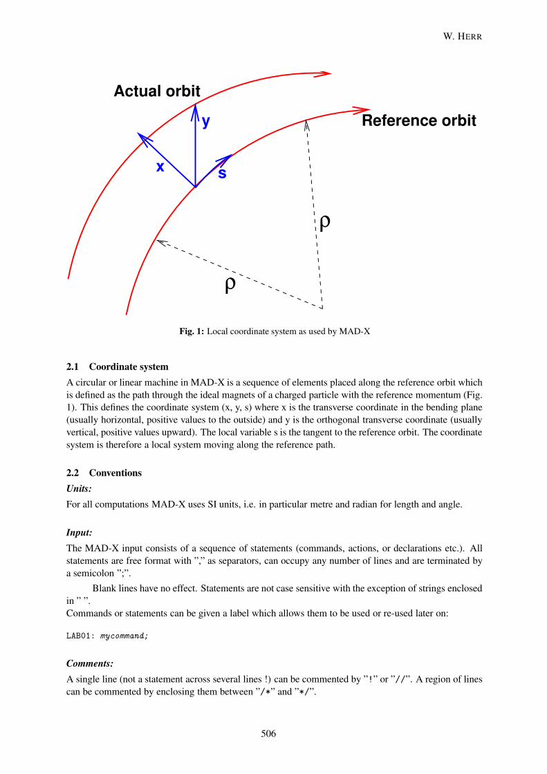
Reference orbit

Actual orbit

ρ

ρ

s

y

x

Fig. 1: Local coordinate system as used by MAD-X

2.1 Coordinate systemA circular or linear machine in MAD-X is a sequence of elements placed along the reference orbit whichis defined as the path through the ideal magnets of a charged particle with the reference momentum (Fig.1). This defines the coordinate system (x, y, s) where x is the transverse coordinate in the bending plane(usually horizontal, positive values to the outside) and y is the orthogonal transverse coordinate (usuallyvertical, positive values upward). The local variable s is the tangent to the reference orbit. The coordinatesystem is therefore a local system moving along the reference path.

2.2 ConventionsUnits:For all computations MAD-X uses SI units, i.e. in particular metre and radian for length and angle.

Input:The MAD-X input consists of a sequence of statements (commands, actions, or declarations etc.). Allstatements are free format with ”,” as separators, can occupy any number of lines and are terminated bya semicolon ”;”.

Blank lines have no effect. Statements are not case sensitive with the exception of strings enclosedin ” ”.Commands or statements can be given a label which allows them to be used or re-used later on:

LAB01: mycommand;

Comments:A single line (not a statement across several lines !) can be commented by ”!” or ”//”. A region of linescan be commented by enclosing them between ”/*” and ”*/”.

2

W. HERR

506

2.3 Variables and expressionsParameter values:Integer or floating point numbers can be assigned to named parameters and can be used in further decla-rations or commands, e.g.:

LENDIP = 8.0;

Various names (keywords used by MAD-X) are protected and cannot be used as variables or labels.

The numerical value of an assignment can be replaced by an expression, e.g.:

LNFX = 6912.00/(NCELL*(4*LBEND + 2*LQUAD));

Expressions:Parameters and variables can be used in expressions, in particular to define dependent quantities. Stan-dard arithmetic operations and functions such as SQRT(), EXP(), trigonometric functions etc. can beused in the expressions as well as random number generators [1]. For instance,

E.g.: ANGLE = 2.0*PI/NBEND;

can compute the bending angle of a dipole, given the total number of bending magnets (nbend). Theconstant PI is predefined in MAD-X, together with many other important constants and particle proper-ties.

Deferred expressions:The usual expressions are evaluated once when the parameter is used, e.g.,

DX = GAUSS()*0.001;

assigns a random number following a Gaussian distribution with a width of 1 mm to the parameter DX.This value is kept in all computations.

A deferred expression is declared by ”:=” instead of ”=” and is evaluated every time the parameteris used, e.g.,

DX := GAUSS()*001;

assigns a different random number everytime the parameter DX is used in the program

The distinction between normal and deferred expressions becomes important for error assignmentand matching.

3 Machine description3.1 Thick and thin elementsFor the calculations, the elements can be defined either as so-called thick lenses with a finite length oras so-called thin lenses with zero length. In the latter case, the effects of an element (e.g., a magnet) onthe beam are represented as impulses (kicks) at a fixed value s on the reference orbit. This simplifiesthe treatment since it allows to treat the machine as a series of linear transformations separated by the”kicks” at the positions of the thin elements. This method is very fast and symplectic by constructionand it is therefore best suited for particle tracking.

The disadvantage is the loss of precision when the magnets are very long (compared to the size ofthe machine) or when fringe fields are important. Part of this precision can be recovered by sub-dividingthe magnets into slices, i.e., shorter sections, each representing a thin lens.

3

A MAD-X PRIMER

507

3.2 Element definitionElements are defined using the concept of element classes. All quadrupoles in a machine belong to theclass QUADRUPOLE. We can define subclasses with different properties with statements like:

MQL: QUADRUPOLE, L=5.0;

MQS: QUADRUPOLE, L=1.5;

where we define two classes (MQL and MQS) of quadrupoles of different length (thick elements). Thedefinitions can be used to define the real quadrupoles such as:

QFL01: MQL; // Focusing quadrupoles

QFS01: MQS;

QDL01: MQL; // Defocusing quadrupoles

QDS01: MQS;

The quadrupoles defined like this inherit all properties of the class unless they are specified explicitly, inwhich case they are overwritten. All numerical attributes in a class definition can be expressions.

Dipole magnets can be defined as rectangular (RBEND) or sector (SBEND) bending magnets, e.g.,

MBL: RBEND, L=14.3;

MBS: RBEND, L=5.0;

The length of a rectangular bending magnet is by default the arc length. All details on the definition ofbending magnets are found in the reference manual [1].

3.3 Element strength definition3.3.1 DipolesThe strength of a bending magnet is specified by the bending angle or alternatively the dipole coefficientk0:

k0 =1

p/cBy [ in T ]

[=

1

ρ=

anglel

][ in rad/m ]

In the latter case, a finite length must be specified.

The definition for a dipole magnet is:

MB001: RBEND, L=14.3, ANGLE=2*PI/1132; //Total number of dipoles is 1132

or, alternatively:

MB001: MBL, ANGLE=2*PI/1132; //Total number of dipoles is 1132

using the defined sub-class.

3.3.2 QuadrupolesWe define a quadrupole by its quadrupole coefficient k1, which is defined as:

k1 =1

p/c

δByδx

[ in T/m ]

[=

1

l · f

]

We define quadrupoles as:

QF007: QUADRUPOLE, L=5.0, K1 = +0.00147235;

QD007: QUADRUPOLE, L=5.0, K1 = -0.00147235;

or using sub-classes:

QF007: QFL, K1 = +0.00147235;

QD007: QDL, K1 = -0.00147235;

4

W. HERR

508

3.3.3 SextupolesHigher order multipoles such as sextupoles we can define as:

SF007: SEXTUPOLE, L=1.4, K2 = +0.00147235;

with:

k2 =1

p/c

δ2Byδ2x

[in T/m2 ]

3.3.4 Orbit correctorsOrbit correction dipoles are identified by the keyword KICKER. The strength of an orbit corrector is thedeflection angle (KICK) measured in rad. Valid definitions are:

LKICK = 0.1;

MCV01: VKICKER, L=0.1, KICK:=KCV01;

MCV02: VKICKER, L=LKICK, KICK:=KCV02;

MCH01: HKICKER, L=LKICK, KICK:=KCH01;

MC001: KICKER, L=0.1, VKICK:=KXV001, HKICK:=KXH001;

The class VKICKER or HKICKER refer to orbit correctors for the vertical and horizontal planes respectively.The attribute KICK refers to the corresponding plane only. The single class KICKER can be used to specifyorbit correctors for both planes. In that case, two attributes HKICK and VKICK are needed to separate thefunctions in the two planes.

In the above example, the correctors and their strengths are given individual names which allowsto set them explicitly to independent values. For the standard orbit correction with MAD-X this ishowever not always necessary. The declarations of the kicks as deferred expressions allows the kicks tobe changed explicitly or by the program.

3.4 MultipolesA special class of elements is defined with the keyword MULTIPOLE. These are general elements ofzero length (thin lenses) and can be used with one or more components of any order. All thin elementscan be written as multipoles in the form:

MPM: MULTIPOLE;

MPLE01: MPM, LRAD=0.0, TILT=angle,

KNL={k n0L, k n1L, k n2L, k n3L,....},KSL={k s0L, k s1L, k s2L, k s3L,....};

The components KNL and KSL are the normal and skew components of the multipole multiplied by therelevant magnetic length. Note that the strength definitions are position dependent, therefore leadingzeroes must be filled for components that do not exist. The attribute LRAD is a fictitious length, which isonly used to compute synchrotron radiation effects. For the computation of lattice functions etc., it canbe set to some dummy value.

Using multipoles, a thin quadrupole can be defined as:

QFT: MPM, LRAD=0, KNL={0, k n1L, 0, 0 };

The thin lens version of a dipole would be written as:

MBT: MPM, LRAD=0, KNL={k n0L, 0, 0, 0 };

5

A MAD-X PRIMER

509

3.5 MarkersThe element class MARKER is used to insert an inactive element at a position s for later use, e.g., as areference. The syntax is:

START_IP: MARKER, AT = 1839.872;

If present in a sequence, the lattice functions are calculated at their positions and they play an importantrole for matching.

A complete list of keywords and pre-defined element classes is found in the reference manual [1].

3.6 Element position in a SEQUENCE

The representation of the machine is called a sequence. It defines the order in which the elements appearin the accelerator or beam line. In a simple case, a sequence can be defined like:

seq_name: SEQUENCE, REFER=CENTRE, LENGTH=6912.00;

...

...

MQF05 : MQL, AT = 256.0000;

BPMH05 : MONITOR, AT = 1.75, FROM=MQF05;

MCH05 : HKICKER, AT = 2.10, FROM=MQF05;

MBL05.002: MBL, AT = 265.9000;

MBL05.002: MBL, AT = 278.1000;

MQD05 : MQL, AT = 288.0000;

BPMV05 : MONITOR, AT = 1.75, FROM=MQD05;

MCV05 : VKICKER, AT = 2.10, FROM=MQD05;

MBL05.003: MBL, AT = 297.9000;

MBL05.004: MBL, AT = 310.1000;

...

...

ENDSEQUENCE;

The keywords SEQUENCE and ENDSEQUENCE define the beginning and end of the definition and the se-quence is assigned a name seq name.

The statements look familiar and the additional attribute AT defines the position relative to thebeginning of the sequence. A position relative to an existing element can be assigned with the FROM

attribute. The total LENGTH of the sequence is specified on the header line of the sequence. The positionscan be defined at the CENTRE, ENTRY or EXIT of an element, indicated by the REFER attribute. The namesgiven to the elements must be unique, i.e., must not appear twice in the same sequence.

Several sequences with different names can be defined in the same file.

In the example above we have assigned the position to named elements. A second possibility is touse class names like in:

...

MBL: MBL, AT = 278.1000;

MQD: MQD, AT = 288.0000;

BPM: BPM, AT = 1.75, FROM=MQD05;

MCV: MCV, AT = 2.10, FROM=MQD05;

MBL: MBL, AT = 297.9000;

MBL: MBL, AT = 310.1000;

...

assuming BPM, MCV, etc. have been defined as classes before. In this case all elements have the samename which is the name of the class and they cannot be distinguished by name.

6

W. HERR

510

Finally, a previously defined sequence can be inserted, allowing the possibility to nest sequences.Example 1 in Appendix A defines a complete machine using the commands already discussed up to now.The dipoles are defined as thin elements whereas the quadrupoles and sextupoles have a finite length.

3.7 Using repetitive definition for periodic machinesThe sequence of a periodic machine or the periodic part of a machine can be defined using the MAD-Xmacro commands. After the usual definition of the cell length lcell, the half length of a quadrupolelquad2 and the number of cells ncell, the whole machine can be defined with a while-loop:

n = 1;

while (n < ncell+1) {

qf: qf, at=(n-1)*lcell+lquad2;

lsf: lsf, at=(n-1)*lcell+lquad2+2.5;

ch: ch, at=(n-1)*lcell+lquad2+3.1;

bpm: bpm, at=(n-1)*lcell+lquad2+3.2;

mbsps: mbsps, at=(n-1)*lcell+lquad2+3.50;




qd: qd, at=(n-1)*lcell+lquad2+32.00;

lsd: lsd, at=(n-1)*lcell+lquad2+34.50;

cv: cv, at=(n-1)*lcell+lquad2+35.10;






n = n + 1;

}

The two types of sequence definitions are entirely equivalent.

A complete definition using this technique is given in example 2 in Appendix B The MAD-Xcommands and the resulting output are identical to example 1 (Appendix A).

4 MAD-X commandsIn addition to the statements which are used to define a machine, the MAD-X commands are used to de-fine and execute actions on the machines, e.g. calculations of Twiss functions, I/O of the lattices, particletracking etc.. An important part of the design procedure is lattice matching, i.e. to vary element param-eters to make machine properties (e.g., Twiss functions) assuming defined values at specified positions(e.g., interaction points, etc.). A complete description of all MAD-X commands is found in [1]. Here Ishall list the most important commands which are necessary to do the basic calculations.

4.1 BEAM commandSome of the MAD-X actions require the knowledge of the beam properties. They are defined with theBEAM command:

BEAM, PARTICLE=name, ENERGY=xxx, SEQUENCE=sname;

The name of the particle type can be given as well as the particle’s energy. The properties (e.g., mass andcharge) of the most important particles are known to MAD-X. Alternatively, the mass and charge can bespecified with MASS = and CHARGE = . When the SEQUENCE attribute is given, it will assign the beam

7

A MAD-X PRIMER

511

only to this particular sequence, otherwise to the active sequence. A complete list of all possible beamquantities is found in [1].

4.2 Input definitionMAD-X statements and commands can be given on the standard input or can be read from a file with:

CALL,FILE="filename";

This file can contain one or more sequences, part of a sequence or commands and is inserted at theposition of the call.

After a sequence has been read, it can be used with:

USE, PERIOD=sname;

This command will expand the specified sequence, insert the drift spaces and make it active.

4.3 MAD-X actionsMAD-X actions are executed to perform operations on the available machines. To calculate the linearlattice functions (Twiss parameters) around the machine, the action:

TWISS;

must be executed, which operates on the sequence defined in the last USE command. However, a sequencecan be specified explicitly on the Twiss command. A summary table is given after execution.

4.4 MAD-X outputThe TWISS command can be modified to specify the wanted output:

SELECT,FLAG=TWISS,COLUMN=NAME,S,MUX,BETX,MUY,BETY;

TWISS,FILE="twiss.out";

In the SELECT command the lattice functions wanted can be specified before TWISS is executed. The fulllist of the lattice functions is given in [1]. The lattice functions are written into the file ”twiss.out”.

The SELECT command can be used to restrict the output to only a range or type of elements:

SELECT,FLAG=TWISS,RANGE=beg/end;

or:

SELECT,FLAG=TWISS,PATTERN="ˆQ.*";

The first will output the lattice functions only within the specified range and the second would restrict theoutput to all elements starting with the specified pattern in the element name. The SELECT commandsact for the desired action (FLAG=) and can be accumulated or overwritten.

4.5 MAD-X graphical outputMAD-X has an builtin graphics package. To plot lattice functions for example, the command sequence:

SELECT,FLAG=TWISS;

TWISS,FILE="twiss.beta";

PLOT, HAXIS=S, VAXIS=BETX, BETY;

may be used to plot the horizontal and vertical β-functions as a function of the position s. The RANGE

attribute can be used with the PLOT command. An output file and a PostScript file are written simultane-ously. For details and all options see [1].

8

W. HERR

512

4.6 MAD-X exampleIn the second part of example 1 the necessary MAD-X commands are given to calculated the latticefunctions with the TWISS command, write them onto a file and plot them in postscript format. At theeand of the execution of a TWISS command, a summary table is printed:

++++++ table: summ

length orbit5 alfa gammatr

6.9120000e+03 -0.0000000e+00 1.6807003e-03 2.4392418e+01

q1 dq1 betxmax dxmax

2.6580000e+01 -3.3561557e+01 1.0754431e+02 2.5680113e+00

dxrms xcomax xcorms q2

1.9304378e+00 0.0000000e+00 0.0000000e+00 2.6620000e+01

dq2 betymax dymax dyrms

-3.3598479e+01 1.0749730e+02 0.0000000e+00 0.0000000e+00

ycomax ycorms deltap

0.0000000e+00 0.0000000e+00 0.0000000e+00

The main parameters of the lattice are summarized in this table, such as horizontal and vertical tunes (Q1,Q2), chromaticities (DQ1, DQ2), etc.

The lattice functions βx and Dx are plotted by the above command sequence as shown in Fig. 2.

The functions are plotted between the 10th and 16th quadrupole of the class QD as specified in theRANGE attribute.

As requested, the lattice functions are written to a file ”twiss.out” and its format is shown in thelast part of Appendix A. At the beginning of this file the basic parameters are summarized again.

5 Matching with MAD-XThe adjustment of machine properties, i.e., matching, is a vital part of the design process and a detaildescription is beyond the scope of this introduction. However some very basic features will be demon-strated by some examples. A basic tutorial on some matching techniques is found in [3, 4].

5.1 Global matchingSome global machine parameters such as tune or chromaticity can be adjusted by global matching. Thefollowing two example are used as a demonstration:

MATCH, SEQUENCE=CASSPS;

VARY,NAME=KQF, STEP=0.00001;

VARY,NAME=KQD, STEP=0.00001;

GLOBAL,SEQUENCE=CASSPS,Q1=26.58;

GLOBAL,SEQUENCE=CASSPS,Q2=26.62;

LMDIF, CALLS=10, TOLERANCE=1.0E-21;

ENDMATCH;

MATCH, SEQUENCE=CASSPS;

VARY,NAME=KSF, STEP=0.00001;

VARY,NAME=KSD, STEP=0.00001;

GLOBAL,SEQUENCE=CASSPS,DQ1=0.0;

GLOBAL,SEQUENCE=CASSPS,DQ2=0.0;


ENDMATCH;

9

A MAD-X PRIMER

513

600. 700. 800. 900. 1000.s (m)

s

10.

20.

30.

40.

50.

60.

70.

80.

90.

100.

110.βx

(m),

βy(m

)

600. 1000. 1400. 1800. 2200.s (m)

s MAD-X 1.11 23/10/03 11.36.14

1.2

1.4

1.6

1.8

2.0

2.2

2.4

2.6

Dx(m

)

Fig. 2: Lattice functions computed and plotted by MAD-X

10

W. HERR

514

The matching attributes and commands are enclosed beteen the MATCH and ENDMATCH statements. Thedesired sequence can be specified. In the first example the global horizontal and vertical tunes arematched to the desired values. The strengths of the main quadrupoles (KQF and KQD) are varied inthe procedure. In the second example the global chromaticities are match to zero, by variation of the sex-tupole strengths KSF and KSD Other attributes control the method used and the quality of the procedure.The new values of the strengths are now associated with the sequence. The following execution of theTWISS command would therefore produce the new parameters.

NOTE: the latter is only true when the quadrupole strengths are defined using deferred expres-sions, i.e.,

QF: QUADRUPOLE, K1:=KQF;

Otherwise the new strengths KQF and KQD are calculated all right, but not assigned to the elements,i.e., they will not be used in subsequent calculations, e.g., computing lattice functions with the TWISS

command.

5.2 Local and insertion matchingProbably the most important matching procedures are those which are used to modify the lattice locally,e.g., for inserting non-periodic regions for experiments, collimation systems etc. In order to avoid adistortion of other parts of the machine, the matching must be restricted to the local region and additionalconstraints must ensure the smooth continuation into the periodic part of the machine.

The example below is a simple matching of a symmetric low β-insertion using four independentquadrupoles. The matching is restricted to the range between the elements left and right where thenormal lattice parameters are given as constraints. For more details on this example see [4].

MATCH, SEQUENCE=CASCELL5,RANGE=LEFT/RIGHT,BETX=28.2,BETY=87.0;

VARY,NAME=KQ1.L, STEP=0.00001;




CONSTRAINT,RANGE=RIGHT,SEQUENCE=CASCELL5,BETX=28.2,BETY=87.0;

CONSTRAINT,RANGE=IP,SEQUENCE=CASCELL5,BETX=10.0,BETY=1.0;


ENDMATCH;

6 Error definitionDuring the design process of a machine it becomes important to test it against imperfections. For thatpurpose, alignment and field errors can be assigned to all machine elements. The calculations will takethese imperfections into account and correction procedures (e.g. orbit correction) are available in MAD-X to test possible correction strategies.

6.1 Alignment errorsThe elements in a machine can be misaligned with the available MAD-X error actions. The commandsequence:

SELECT, FLAG= ERROR, CLASS=MQ;

EALIGN, DX:=GAUSS()*0.0005; DY:=GAUSS()*0.0002;

assigns alignment errors to all quadrupoles belonging to the class MQ with a r.m.s. value of 0.5 mm in thehorizontal and 0.2 mm in the vertical plane, both following a Gaussian distribution. In that case again the

11

A MAD-X PRIMER

515

use of deferred expressions is of utmost importance. To assign the errors, the program steps through thesequence and for every element of the selected class the corresponding misalignments DX and DY areevaluated each time. Using the standard expression, the misalignments DX and DY are calculated onceand all elements of the selected class get the same error. For a complete list of all misalignment optionssee [1].

6.2 Field errorsThe program allows to assign field errors of any order to the machine elements with commands like:

SELECT, FLAG= ERROR, CLASS=MB;

EFCOMP, RADIUS:=0.017, ORDER:=0,

DKNR:={0,0,GAUSS()*7E-4,GAUSS()*1E-4,0,0},

DKSR:={0,0,GAUSS()*3E-4,GAUSS()*6E-4,0,0},

In this example normal and skew field errors (sextupole and octupole) are assigned to dipole magnets ofthe class MB. It is possible to assign absolute or relative field errors, the latter normalized to the strengthof the corresponding element. The RADIUS (reference for the measurement) and ORDER control thisbehaviour. For a detailed discussion see [1].

7 Orbit correctionA misaligned machine can be corrected using the MAD-X orbit correction procedures [5]. The inputdata is taken from the last TWISS table, i.e., TWISS must run before a correction can be executed.

Very basic closed orbit correction statements are of the form:

CORRECT, PLANE=X, NCORR=20, ERROR=1.0E-04;

or

CORRECT, MODE=SVD;

For all details and options see [1, 5].

8 Advanced options and commandsMAD-X has many more features and commands for advanced design and evaluation of accelerator lat-tices. Most prominent are the evaluation of beam parameters (in case of radiation), geometrical survey,tracking and physical and dynamic aperture determination. However, a full description is well beyondthe scope of this simplified introduction. To get a flavour, I shall give two examples, one for a simpletracking and another for the advanced use of macros.

8.1 Particle trackingThe example shown below demonstrates particle tracking in MAD-X. It shows the simultaneous trackingof 20 particles in horizontal phase space where the particles are distributed on a circle in x–px phasespace. All commands are enclosed between the keywords TRACK and ENDTRACK. The initial coordinatesof the particles are assigned with the command START and the tracking is executed with RUN.

Tracking in MAD-X is possible using thin lenses. A lattice defined with thick elements has to beconverted to thin lenses with the command MAKETHIN before the tracking can be done. For details on thecommand MAKETHIN consult the reference manual [1].

12

W. HERR

516

MAKETHIN,SEQUENCE=CASSPS;

USE,SEQUENCE=CASSPS;

TRACK;

NSTEP = 20;

RAD = 100.0E-06;

ANGSTP = 2*PI/NSTEP;

N = 0;

WHILE(N <= NSTEP) {

ANG = N*ANGSTP;

XS = RAD*COS(ANG);

XPS = RAD*SIN(ANG);

VALUE, XS,XPS;

START,X=XS,PX=XPS;

N = N + 1;

}

RUN,TURNS=1024;

ENDTRACK;

STOP;

The use of tracking may require additional attributes in the BEAM command. The above example showsthe power of the input language.

8.2 Use of macrosThe power of the MAD-X input language is further enhanced by the use of macros. For illustration,example 2 in Appendix B has been modified. For some cases, it is required that the elements havedistinct names, (e.g., where all elements must be treated as separate objects, such as orbit corrections).This can be easily done by editing example 1, where every element is listed on a separate line. Editingthe example 2 with the while loop would fail because two elements must not have the same name. Usingthe macro language, the while loop can be modified like in example 3 in Appendix C. The definition ofa cell is now done within the subroutine inst. This subroutine takes input parameters from the callingMAD-input and most important, can change the names of the elements, using the input information. Theresult of this scheme is the same as before, however the orbit correctors, their corresponding strengthparameters and the beam position monitors are now numbered sequentially. A MAD-X input file andthe corresponding Twiss output are shown in the second part of example 3. The increasing sequencenumbers as part of the element names are now clearly visible. In this example the quadrupoles havebeen misaligned in the two planes following a Gaussian distribution with 0.1 mm and 0.2 mm r.m.s.respectivly.

Therefore the horizontal and vertical orbit is distorted and the maximum and r.m.s. values can befound in the Twiss summary table.

9 How to run MAD-X ?MAD-X can be run either interactively or in batch mode.

9.1 Interactive modeTo run MAD-X interactively, one can execute MAD-X and input the commands and statements in thecommand line of the standard input.

Alternatively, one or more files with commands and statements can be read using the command:

CALL,FILE="filename";

13

A MAD-X PRIMER

517

9.2 Batch modeMAD-X can be run as a background of batch program by redirecting an input file into the MAD-Xstandard input. For UNIX (LINUX) like:

madx < inputfile

The output is normally send to the standard output, unless it is redirected.

AppendicesThe appendices list examples which are referenced in the text. For all cases the sequence definition isgiven in the first part and a MAD-X input file to use the sequence is displayed in the second part of eachexample.

A Example 1, Simplest caseA.1 Sequence definition// define the total length

circum=6912.00;

// define number of cells and therefore cell length

ncell = 108;

lcell = circum/ncell;

// define lengths of elements and half lengths

lquad = 3.085;

lmb = 6.260;

lsex = 1.0;

// forces and other constants;

// element definitions;

// define bending magnet as multipole

mbsps: multipole, lrad=dummy, knl={2.0*pi/(8*ncell)};

// define quadrupole and their strengths

qsps: quadrupole, l=lquad;

qf: qsps, k1:=kqf;

qd: qsps, k1:=kqd;

kqf = 1.4631475E-02;

kqd = -1.4643443E-02;

// define sextupoles for chromaticity correction

lsf: sextupole, l=lsex,k2:=ksf;

lsd: sextupole, l=lsex,k2:=ksd;

ksf = 2.0284442E-02;

ksd = -3.8394267E-02;

// define orbit correctors and beam position monitors

bpm: monitor, l=0.1;

ch: hkicker, l=0.1;

cv: vkicker, l=0.1;

cassps: sequence, refer=centre, l = circum;

start_machine: marker, at = 0;

14

W. HERR

518

qf, at = 1.5425;

lsf, at = 4.0425;

ch, at = 4.6425;

bpm, at = 4.7425;

mbsps, at = 5.0425;

mbsps, at = 11.4425;

mbsps, at = 23.6425;

mbsps, at = 30.0425;

qd, at = 33.5425;

lsd, at = 36.0425;

cv, at = 36.6425;

bpm, at = 36.7425;

mbsps, at = 37.0425;

mbsps, at = 43.4425;

mbsps, at = 55.6425;

mbsps, at = 62.0425;

qf, at = 65.5425;

lsf, at = 68.0425;

ch, at = 68.6425;

bpm, at = 68.7425;

mbsps, at = 69.0425;

mbsps, at = 75.4425;

mbsps, at = 87.6425;

mbsps, at = 94.0425;

qd, at = 97.5425;

lsd, at = 100.0425;

cv, at = 100.6425;

bpm, at = 100.7425;

mbsps, at = 101.0425;

mbsps, at = 107.4425;

mbsps, at = 119.6425;

mbsps, at = 126.0425;

qf, at = 129.5425;

lsf, at = 132.0425;

ch, at = 132.6425;

bpm, at = 132.7425;

mbsps, at = 133.0425;

mbsps, at = 139.4425;

mbsps, at = 151.6425;

mbsps, at = 158.0425;

qd, at = 161.5425;

lsd, at = 164.0425;

cv, at = 164.6425;

bpm, at = 164.7425;

mbsps, at = 165.0425;

mbsps, at = 171.4425;

...

mbsps, at = 6775.6425;

mbsps, at = 6782.0425;

qf, at = 6785.5425;

lsf, at = 6788.0425;

ch, at = 6788.6425;

bpm, at = 6788.7425;

mbsps, at = 6789.0425;

mbsps, at = 6795.4425;

mbsps, at = 6807.6425;

15

A MAD-X PRIMER

519

mbsps, at = 6814.0425;

qd, at = 6817.5425;

lsd, at = 6820.0425;

cv, at = 6820.6425;

bpm, at = 6820.7425;

mbsps, at = 6821.0425;

mbsps, at = 6827.4425;

mbsps, at = 6839.6425;

mbsps, at = 6846.0425;

qf, at = 6849.5425;

lsf, at = 6852.0425;

ch, at = 6852.6425;

bpm, at = 6852.7425;

mbsps, at = 6853.0425;

mbsps, at = 6859.4425;

mbsps, at = 6871.6425;

mbsps, at = 6878.0425;

qd, at = 6881.5425;

lsd, at = 6884.0425;

cv, at = 6884.6425;

bpm, at = 6884.7425;

mbsps, at = 6885.0425;

mbsps, at = 6891.4425;

mbsps, at = 6903.6425;

mbsps, at = 6910.0425;

end_machine: marker, at = 6912.00;

endsequence;

A.2 MAD-X directivesTITLE, s=’MAD-X test’;

// Read input file with machine description

call file="spsall.seq";

option,-echo;

// Define the beam for the machine

Beam, particle = proton, sequence=cassps, energy = 450.0;

// Use the sequence with the name: cassps

use, period=cassps;

// Define the type and amount of output for the action TWISS

select,flag=twiss,column=name,s,x,y,mux,betx,muy,bety,dx,dy;

// Execute the Twiss command to calculate the Twiss parameters

// Compute at the centres of the elements and write to: twiss.out

twiss,centre,file=twiss.out;

// Plot the horizontal and vertical beta function between the

// 10th and 16th occurence of a defocussing quadrupole

plot, haxis=s, vaxis=x, betx, bety,colour=100,

range=qd[10]/qd[16];

plot, haxis=s, vaxis=dx, colour=100,

range=qd[10]/qd[36];

stop;

16

W. HERR

520

A.3 TWISS summary table++++++ table: summ


6.9120000e+03 -0.0000000e+00 1.6807003e-03 2.4392418e+01


2.6580000e+01 -3.3561557e+01 1.0754431e+02 2.5680113e+00


1.9304378e+00 0.0000000e+00 0.0000000e+00 2.6620000e+01


-3.3598479e+01 1.0749730e+02 0.0000000e+00 0.0000000e+00


0.0000000e+00 0.0000000e+00 0.0000000e+00

A.4 TWISS lattice functions written to the file ”twiss.out”@ NAME %05s "TWISS"

@ TYPE %05s "TWISS"

@ SEQUENCE %06s "CASSPS"

@ PARTICLE %06s "PROTON"

@ MASS %le 0.938271998

@ CHARGE %le 1

@ ENERGY %le 450

@ PC %le 449.999021827

@ GAMMA %le 479.605062241

@ KBUNCH %le 1

@ BCURRENT %le 0

@ SIGE %le 0

@ SIGT %le 0

@ NPART %le 0

@ EX %le 1

@ EY %le 1

@ ET %le 1

@ LENGTH %le 6912

@ ALFA %le 0.00168070032886

@ ORBIT5 %le -0

@ GAMMATR %le 24.3924182122

@ Q1 %le 26.58

@ Q2 %le 26.62

@ DQ1 %le -33.5615573373

@ DQ2 %le -33.5984799903

@ DXMAX %le 2.5680113011

@ DYMAX %le 0

@ XCOMAX %le 0

@ YCOMAX %le 0

@ BETXMAX %le 107.544319159

@ BETYMAX %le 107.497305443

@ XCORMS %le 0

@ YCORMS %le 0

@ DXRMS %le 1.93043782638

@ DYRMS %le 0

@ DELTAP %le 0

17

A MAD-X PRIMER

521

@ TITLE %01s "s"

@ ORIGIN %16s "MAD-X 1.11 Linux"

@ DATE %08s "23/10/03"

@ TIME %08s "11.36.14"

* NAME S BETX DX

$ %s %le %le %le

"CASSPS$START" 0 103.8655173 2.523441048

"START_MACHINE" 0 103.8655173 2.523441048

"QF" 1.5425 107.5443192 2.568011301

"DRIFT_0" 3.11375 103.7300292 2.521784419

"LSF" 3.6425 101.2568359 2.491316849

"DRIFT_1" 4.5925 96.90195183 2.43657606

"MBSPS" 5.0425 94.87888064 2.410646213

"DRIFT_2" 8.2425 81.22989411 2.249527296

"MBSPS" 11.4425 68.87370326 2.08840838

"DRIFT_3" 17.5425 48.90078374 1.825635993

"MBSPS" 23.6425 33.62561103 1.562863606

"DRIFT_2" 26.8425 27.4909994 1.448286904

"MBSPS" 30.0425 22.64918345 1.333710202

"DRIFT_4" 31.02125 21.42644598 1.305783529

"QD" 33.5425 19.51348873 1.255914454

"DRIFT_0" 35.11375 20.35528979 1.278677181

"LSD" 35.6425 20.93741261 1.293764004

"DRIFT_1" 36.5925 22.07198555 1.320870352

"MBSPS" 37.0425 22.64918345 1.333710202

"DRIFT_2" 40.2425 27.4909994 1.448286904

"MBSPS" 43.4425 33.62561103 1.562863606

"DRIFT_3" 49.5425 48.90078374 1.825635993

"MBSPS" 55.6425 68.87370326 2.08840838

"DRIFT_2" 58.8425 81.22989411 2.249527296

"MBSPS" 62.0425 94.87888064 2.410646213

"DRIFT_4" 63.02125 99.31172846 2.467043631

"QF" 65.5425 107.5443192 2.568011301

"DRIFT_0" 67.11375 103.7300292 2.521784419

"LSF" 67.6425 101.2568359 2.491316849

"DRIFT_1" 68.5925 96.90195183 2.43657606

"MBSPS" 69.0425 94.87888064 2.410646213

"DRIFT_2" 72.2425 81.22989411 2.249527296

"MBSPS" 75.4425 68.87370326 2.08840838

"DRIFT_3" 81.5425 48.90078374 1.825635993

"MBSPS" 87.6425 33.62561103 1.562863606

"DRIFT_2" 90.8425 27.4909994 1.448286904

"MBSPS" 94.0425 22.64918345 1.333710202

"DRIFT_4" 95.02125 21.42644598 1.305783529

"QD" 97.5425 19.51348873 1.255914454

"DRIFT_0" 99.11375 20.35528979 1.278677181

"LSD" 99.6425 20.93741261 1.293764004

"DRIFT_1" 100.5925 22.07198555 1.320870352

"MBSPS" 101.0425 22.64918345 1.333710202

"DRIFT_2" 104.2425 27.4909994 1.448286904

"MBSPS" 107.4425 33.62561103 1.562863606

"DRIFT_3" 113.5425 48.90078374 1.825635993

"MBSPS" 119.6425 68.87370326 2.08840838

"DRIFT_2" 122.8425 81.22989411 2.249527296

"MBSPS" 126.0425 94.87888064 2.410646213

"DRIFT_4" 127.02125 99.31172846 2.467043631

18

W. HERR

522

"QF" 129.5425 107.5443192 2.568011301

.........

.........

.........

B Example 2, Use of WHILE commandB.1 Sequence definition// define the total length

circum=6912.0;


ncell = 108;



lquad = 3.085;

lquad2 = lquad/2.;

lsex = 1.0;




mbsps: multipole, lrad=dummy, knl={2.0*pi/(8*ncell)};



qf: qsps, k1:=kqf;

qd: qsps, k1:=kqd;

kqf = 1.4631475E-02;

kqd = -1.4643443E-02;




ksf = 2.0284442E-02;

ksd = -3.8394267E-02;



ch: hkicker, l=0.1;

cv: vkicker, l=0.1;

// sequence declaration;

cassps: sequence, refer=centre, l:=circum;


// This defines ONE cell, repeat NCELL times

// to get the full machine

// SPS has 8 bending magnets per cell

n = 1;




ch: ch, at=(n-1)*lcell+lquad2+3.1;

19

A MAD-X PRIMER

523








cv: cv, at=(n-1)*lcell+lquad2+35.10;






n = n + 1;

}

end_machine: marker at=circum;

endsequence;

C Example 3, Use of MAD-X macros and imperfectionsC.1 Sequence definition// define a subroutine "inst" to insert elements

// with numbering

// all strings "nx" in the macro are replaced by

// the input value of nx.

inst(nx,n,lcell,lquad2): macro = {



chnx: hkicker,l=0.0,kick:=kchnx,

at=(n-1)*lcell+lquad2+3.1;

bpmhnx: monitor,l=0.0,








cvnx: vkicker,l=0.0,kick:=kcvnx,


bpmvnx: monitor,l=0.0,






n = n + 1;

}

// define the total length

circum=6912.0;


ncell = 108;

20

W. HERR

524



lquad = 3.085;

lquad2 = lquad/2.;

lquad3 = 0.0;

lmb = 6.260;

lmb2 = lmb/2.;

lsex = 1.0;




mbsps: multipole, lrad=dummy, l=lmb, knl={2.0*pi/(8*ncell)};



qf: qsps, k1:=kqf;

qd: qsps, k1:=kqd;

kqf = 1.4631475E-02;

kqd = -1.4643443E-02;




ksf = 2.0284442E-02;

ksd = -3.8394267E-02;



ch: hkicker, l=0.1;

cv: vkicker, l=0.1;

// sequence declaration;

cassps: sequence, refer=centre, l=circum;


// This defines ONE cell, repeat NCELL times

// to get the full machine

// SPS has 8 bending magnets per cell

n = 1;


// here we call the macro, cell number n is argument

// and used for numbering the elements

exec inst($n,n,lcell,lquad2);

}

end_machine: marker at=circum;

endsequence;

C.2 MAD-X directivesTITLE, s=’MAD-X test’;

// Read input file with machine description

// This machine is constructed with macro

// subroutine INST()

21

A MAD-X PRIMER

525

call file="spsmac.seq";

option,-echo;

// Define the beam for the machine

Beam, particle = proton, sequence=cassps, energy = 450.0;

// Use the sequence with the name: cassps

use, sequence=cassps;

eoption,add=false,seed=62971100;

select,flag=error,pattern="q.*";

ealign,dx:=tgauss(3.0)*1.0e-4,dy:=tgauss(3.0)*2.0e-4;

eprint;

// Define the type and amount of output

select,flag=twiss,class=monitor,column=name,s,x,betx;

select,flag=twiss,class=vkicker,column=name,s,x,betx;

select,flag=twiss,class=hkicker,column=name,s,x,betx;

// Execute the Twiss command to calculate the Twiss parameters

// Compute at the centre of the element and write to: twiss.out

twiss,save,centre,file=twiss.out;

stop;

C.3 TWISS summary table++++++ table: summ


6.9120000e+03 -0.0000000e+00 1.6804423e-03 2.4394290e+01


2.6580085e+01 -1.2827690e-04 1.0808509e+02 2.6296100e+00


1.9361006e+00 3.1098580e-03 1.0489137e-03 2.6620213e+01


-5.1039987e-04 1.0787781e+02 4.0349793e-01 1.5327251e-01


8.6691696e-03 2.8727246e-03 0.0000000e+00

C.4 TWISS lattice functions@ NAME %05s "TWISS"

@ TYPE %05s "TWISS"

@ SEQUENCE %06s "CASSPS"

@ PARTICLE %06s "PROTON"

@ MASS %le 0.938271998

@ CHARGE %le 1

@ ENERGY %le 450

@ PC %le 449.999021827

@ GAMMA %le 479.605062241

@ KBUNCH %le 1

@ BCURRENT %le 0

22

W. HERR

526

@ SIGE %le 0

@ SIGT %le 0

@ NPART %le 0

@ EX %le 1

@ EY %le 1

@ ET %le 1

@ LENGTH %le 6912

@ ALFA %le 0.00168044235319

@ ORBIT5 %le -0

@ GAMMATR %le 24.3942904601

@ Q1 %le 26.5800856671

@ Q2 %le 26.6202187135

@ DQ1 %le -0.000128276909332

@ DQ2 %le -0.000510399876937

@ DXMAX %le 2.629610492

@ DYMAX %le 0.403497938523

@ XCOMAX %le 0.00310985806321

@ YCOMAX %le 0.0086691696294

@ BETXMAX %le 108.085099015

@ BETYMAX %le 107.877818541

@ XCORMS %le 0.00104891378772

@ YCORMS %le 0.0028727246142

@ DXRMS %le 1.93610068609

@ DYRMS %le 0.153272554514

@ DELTAP %le 0

@ TITLE %01s "s"

@ ORIGIN %16s "MAD-X 1.11 Linux"

@ DATE %08s "23/10/03"

@ TIME %08s "10.54.36"

* NAME S X BETX

$ %s %le %le %le

"CH1" 4.6425 7.270283965e-05 96.71513054

"BPMH1" 4.7425 7.074377128e-05 96.26414369

"CV1" 36.6425 -0.000609759073 22.16791457

"BPMV1" 36.7425 -0.0006136057601 22.29453352

"CH2" 68.6425 -0.001619774866 96.60029697

"BPMH2" 68.7425 -0.001616493006 96.15012782

"CV2" 100.6425 -0.0006806900062 22.20590744

"BPMV2" 100.7425 -0.0006809745368 22.33285114

"CH3" 132.6425 -0.0006702055164 96.69082398

"BPMH3" 132.7425 -0.0006672287746 96.23936818

"CV3" 164.6425 0.0002920301383 22.11019753

"BPMV3" 164.7425 0.0002953017665 22.23679301

"CH4" 196.6425 0.001157348134 96.6649292

"BPMH4" 196.7425 0.001154759396 96.21335536

"CV4" 228.6425 0.000373991881 22.08455422

"BPMV4" 228.7425 0.0003728320023 22.21117154

"CH5" 260.6425 1.317974197e-05 96.71965263

"BPMH5" 260.7425 1.236758651e-05 96.26877918

"CV5" 292.6425 -0.0002913559575 22.1823912

"BPMV5" 292.7425 -0.0002936789916 22.30912451

"CH6" 324.6425 -0.0009131218543 96.62975425

"BPMH6" 324.7425 -0.0009115133179 96.17889384

"CV6" 356.6425 -0.0004721562615 22.1454883

"BPMV6" 356.7425 -0.0004729356669 22.27221019

"CH7" 388.6425 -0.0006096356393 96.67763938

23

A MAD-X PRIMER

527

"BPMH7" 388.7425 -0.0006068161018 96.22676343

"CV7" 420.6425 0.0003186361334 22.16647139

"BPMV7" 420.7425 0.0003222988135 22.29331691

"CH8" 452.6425 0.001319551812 96.69719699

"BPMH8" 452.7425 0.001317680986 96.2448662

"CV8" 484.6425 0.0008399337545 22.0183191

"BPMV8" 484.7425 0.0008419042414 22.14474739

"CH9" 516.6425 0.00127367779 96.72628201

"BPMH9" 516.7425 0.001269314367 96.27522738

"CV9" 548.6425 -0.0001569946883 22.16736164

"BPMV9" 548.7425 -0.0001625635013 22.29406121

"CH10" 580.6425 -0.001695832426 96.63883761

"BPMH10" 580.7425 -0.001693540175 96.18855903

"CV10" 612.6425 -0.001134640886 22.21084481

"BPMV10" 612.7425 -0.001137909267 22.33761433

"CH11" 644.6425 -0.001891788389 96.60737231

"BPMH11" 644.7425 -0.001885758488 96.15696162

"CV11" 676.6425 2.602143671e-05 22.18437067

"BPMV11" 676.7425 3.164251283e-05 22.31133474

"CH12" 708.6425 0.001604718692 96.724361

"BPMH12" 708.7425 0.001603215697 96.27158303

"CV12" 740.6425 0.00126167154 21.98294563

"BPMV12" 740.7425 0.001264627726 22.10929259

"CH13" 772.6425 0.001934577849 96.74062223

.......

.......

.......

References[1] The MAD-X Home Page, version February 2003,

http://frs.home.cern.ch/frs/Xdoc/mad-X.html.[2] W. Herr, MAD for pedestrian, Presentation at CERN Accelerator School

DESY Zeuthen, 15. - 26. 9. 2003.[3] W. Herr, Course on optics design,

http://cern.ch/werner.herr/COURSE/.[4] O. Bruning and W. Herr, Problems and solutions of the exercises in the optics course,

Course at CERN Accelerator School, DESY Zeuthen, 15. - 26. 9. 2003.[5] W. Herr; Implementation of new orbit correction procedures in the MAD-X program, CERN-SL-

2002-48 (AP) (2002).

24

W. HERR

528

a mad-x primer - cern document servercds.cern.ch/record/744163/files/p505.pdf · 1.1 what is needed...

Documents