a machine learning teaching aid msc development project
TRANSCRIPT

A Machine Learning Teaching AidMSc Development Project
Daryl Weir0508104
Supervisor: Dr Simon Rogers
A dissertation submitted in part fulfilmentof the requirement of the Degree of
Master of Science at The University of Glasgow
September 2010

Abstract
The aim of this project was to develop an application to assist in teach-ing some of the basic concepts of machine learning. This is a subject area atthe intersection of computer science and applied statistics. It offers power-ful techniques for inferring information about huge collections of data, andalgorithms from the field are constantly being applied to new problems in adiverse range of subject areas.
Many of the algorithms involved are quite complicated from a mathe-matical standpoint, but lend themselves well to visualization. To this end,the application produced by the project implements simple two dimensionalcases of a selection of these algorithms and allows users to explore them vi-sually. In addition, it offers sophisticated features for generating data for usewith these algorithms.
The user evaluation carried out at the conclusion of the project showed afavourable reaction to the teaching aid software. Users with machine learningexperience indicated that it represents a powerful didactic tool. It is designedto be modular and easily extensible, so that further algorithms can be addedin the future, further increasing the usefulness of the program to students ofmachine learning.

Acknowledgements
I’d like to take this opportunity to thank a number of people, withoutwhom this project would not have been possible.First and foremost, thanks to my project supervisor, Simon Rogers, for hisinvaluable assistance and insight throughout the past year.Secondly, thanks to Clare and Amanda for keeping me sane over the courseof the MSc IT. It’s been quite a year.Thanks also to everyone who helped test my application and providedvaluable feedback.Last but not least, thanks to my family for supporting me through mystudies.
Daryl WeirSeptember 2010
i

Contents
Acknowledgements i
Table of Contents ii
1 Introduction 1
2 Problem Context 32.1 Implemented Algorithms . . . . . . . . . . . . . . . . . . . . . 3
2.1.1 Supervised Learning . . . . . . . . . . . . . . . . . . . 42.1.2 Unsupervised Learning . . . . . . . . . . . . . . . . . . 82.1.3 Cross Validation . . . . . . . . . . . . . . . . . . . . . 9
3 Survey of Related Software 113.1 Machine Learning Applets . . . . . . . . . . . . . . . . . . . . 11
3.1.1 Regression . . . . . . . . . . . . . . . . . . . . . . . . . 113.1.2 Classification . . . . . . . . . . . . . . . . . . . . . . . 123.1.3 Clustering . . . . . . . . . . . . . . . . . . . . . . . . . 123.1.4 Discussion . . . . . . . . . . . . . . . . . . . . . . . . . 133.1.5 Gaussian Processes . . . . . . . . . . . . . . . . . . . . 13
3.2 Weka and Java-ML . . . . . . . . . . . . . . . . . . . . . . . . 143.3 MATLAB and Octave . . . . . . . . . . . . . . . . . . . . . . 14
3.3.1 MATLAB . . . . . . . . . . . . . . . . . . . . . . . . . 143.3.2 Octave . . . . . . . . . . . . . . . . . . . . . . . . . . . 153.3.3 JavaOctave . . . . . . . . . . . . . . . . . . . . . . . . 15
3.4 Mathematics and Statistics Libraries . . . . . . . . . . . . . . 163.4.1 Apache Commons Math . . . . . . . . . . . . . . . . . 163.4.2 JAMA . . . . . . . . . . . . . . . . . . . . . . . . . . . 16
3.5 Quadratic Programming . . . . . . . . . . . . . . . . . . . . . 173.5.1 LibSVM . . . . . . . . . . . . . . . . . . . . . . . . . . 173.5.2 QuadProjJ . . . . . . . . . . . . . . . . . . . . . . . . 173.5.3 New Implementation . . . . . . . . . . . . . . . . . . . 18
ii
3.6 Plotting . . . . . . . . . . . . . . . . . . . . . . . . . . . . . . 18
4 Requirements 194.1 Requirements Capture Process . . . . . . . . . . . . . . . . . . 194.2 Requirements Overview . . . . . . . . . . . . . . . . . . . . . . 20
5 Analysis and Design 215.1 The Domain Model . . . . . . . . . . . . . . . . . . . . . . . . 21
5.1.1 The data Package . . . . . . . . . . . . . . . . . . . . . 225.1.2 The algorithms Package . . . . . . . . . . . . . . . . . 23
5.2 Graphical User Interface Design . . . . . . . . . . . . . . . . . 265.2.1 Basic Layout . . . . . . . . . . . . . . . . . . . . . . . 275.2.2 Plotting . . . . . . . . . . . . . . . . . . . . . . . . . . 295.2.3 The OptionPanel Class . . . . . . . . . . . . . . . . . . 30
5.3 Modularity . . . . . . . . . . . . . . . . . . . . . . . . . . . . 315.4 Final Design . . . . . . . . . . . . . . . . . . . . . . . . . . . . 31
6 Implementation 336.1 Development Method . . . . . . . . . . . . . . . . . . . . . . . 336.2 First Prototype . . . . . . . . . . . . . . . . . . . . . . . . . . 346.3 Adding Interaction . . . . . . . . . . . . . . . . . . . . . . . . 36
6.3.1 Datapoints and Datasets . . . . . . . . . . . . . . . . . 366.3.2 Adding Points . . . . . . . . . . . . . . . . . . . . . . . 376.3.3 Removing Points . . . . . . . . . . . . . . . . . . . . . 39
6.4 Algorithm Implementation . . . . . . . . . . . . . . . . . . . . 406.4.1 Minimized Loss . . . . . . . . . . . . . . . . . . . . . . 406.4.2 KNN . . . . . . . . . . . . . . . . . . . . . . . . . . . . 436.4.3 K Means . . . . . . . . . . . . . . . . . . . . . . . . . . 436.4.4 SVM . . . . . . . . . . . . . . . . . . . . . . . . . . . . 456.4.5 Kernel K Means . . . . . . . . . . . . . . . . . . . . . . 476.4.6 Maximum Likelihood . . . . . . . . . . . . . . . . . . . 48
6.5 Sampling Data . . . . . . . . . . . . . . . . . . . . . . . . . . 496.5.1 Polynomial Sampling . . . . . . . . . . . . . . . . . . . 496.5.2 Gaussian Sampling . . . . . . . . . . . . . . . . . . . . 506.5.3 Polygon Sampling . . . . . . . . . . . . . . . . . . . . . 50
6.6 Data storage . . . . . . . . . . . . . . . . . . . . . . . . . . . . 516.6.1 Saving/Loading Data . . . . . . . . . . . . . . . . . . . 516.6.2 Example Datasets . . . . . . . . . . . . . . . . . . . . . 526.6.3 Exporting Images . . . . . . . . . . . . . . . . . . . . . 52
iii

7 Testing and Evaluation 537.1 System Testing . . . . . . . . . . . . . . . . . . . . . . . . . . 537.2 User Evaluation . . . . . . . . . . . . . . . . . . . . . . . . . . 55
7.2.1 Methodology . . . . . . . . . . . . . . . . . . . . . . . 557.2.2 Results . . . . . . . . . . . . . . . . . . . . . . . . . . . 56
8 Conclusion 608.1 Project Status . . . . . . . . . . . . . . . . . . . . . . . . . . . 608.2 Outstanding Issues . . . . . . . . . . . . . . . . . . . . . . . . 608.3 Areas for Further Work . . . . . . . . . . . . . . . . . . . . . . 61
A Statement of Requirements 63A.1 Functional Requirements . . . . . . . . . . . . . . . . . . . . . 63A.2 Non-functional Requirements . . . . . . . . . . . . . . . . . . 64A.3 Use Cases . . . . . . . . . . . . . . . . . . . . . . . . . . . . . 64
B Design Documents 66
C Evaluation Documents 72C.1 Basic Information Document . . . . . . . . . . . . . . . . . . . 73C.2 Task List . . . . . . . . . . . . . . . . . . . . . . . . . . . . . . 74C.3 Questionnaire . . . . . . . . . . . . . . . . . . . . . . . . . . . 75
D Dataset file format 77
E Contents of Accompanying CD 78
Bibliography 79
iv

Chapter 1
Introduction
The field of machine learning is a rapidly growing and increasingly importantarea of computing science. As sensing technologies have improved and theprocessing power of computers has continued to grow, a massive amount ofinformation about a vast range of phenomena has been generated. Thanksto commensurate increases in storage capacity, retaining this data is no sig-nificant challenge. However, analysing such a large, unwieldy collection isextremely difficult and no traditional model exists for the task. The primarygoal of machine learning is to develop algorithms which allow information tobe inferred about the underlying behaviour of a system which has generateda set of data. As a result, the term inference is often used interchangablywith machine learning within computing science.
Machine learning has its origins as a subfield of artificial intelligence (AI),where it arose to fulfil the need for systems which could build functional rep-resentations of phenomena based on observed data. Unlike pure AI research,machine learning methodologies are not concerned with understanding thenature of intelligence - their focus is on efficiently and accurately inferring re-lationships, and producing concrete results. For this reason, machine learninghas grown significantly outwith the confines of artificial intelligence, and hasbeen successfully used to model problems in such diverse fields as computervision, information retrieval, biology and stock market analysis.
The subject is a fairly mathematical one, drawing many of its techniquesfrom applied statistics. Hence, it can be an intimidating subject to learnfor computer scientists who do not have a background in mathematics orstatistics. Machine learning models are often expressed in terms of vectorsand matrices representing the parameters, and it is not necessarily intuitivewhat changing these parameters will do to the solution. However, manymachine learning concepts lend themselves very easily to visualization. Forexample, a common problem in the field is regression. This seeks to model
1

the relationship between a dependent variable and one or more independentvariables. In the case where there is only one independent variable, the modelis simply a planar curve. The effect of altering the parameters can readilybe seen by observing how this curve changes.
The School of Computing Science at the University of Glasgow offersan elective in machine learning. In the current format of this course, labsessions involve the use of MATLAB [16], a powerful numerical computingenvironment. While it is possible to implement a wide variety of machinelearning algorithms using the MATLAB scripting language, it is often noteasy or intuitive to do so. Additionally, most students taking the course havelittle to no experience of the software and so they must spend time learningthe basics of the language and following step by step examples rather thanfocusing on improving their machine learning knowledge. This is not an idealteaching situation, particularly given that lab slots are limited.
The aim of this project was to produce a teaching aid application whichtook advantage of the ease of visualization of a variety of machine learningalgorithms to allow users to experiment directly with the effects of changingdata and, where appropriate, parameters on the output of these algorithms.The software is intended to be used in lab sessions to reinforce students’ un-derstanding of the concepts they have already seen in lectures. The teachingaid allows the user to plot data in two dimensional space using a variety oftechniques, and then train an algorithm on that data and observe the output.
As well as its usefulness in a lab setting, the teaching aid can also beused in lectures to interactively demonstrate new algorithms as they areencountered in the notes. This is more useful than a series of static slides fordemonstrating purposes, and can still be done fairly quickly. It is currentlytime consuming and impractical to describe and run MATLAB scripts in thelectures, whereas using the teaching aid the lecturer can quickly and easilyillustrate the effect of successive iterations or parameter changes in a varietyof algorithms.
The remainder of this document will discuss the development of the teach-ing aid in detail.
2

Chapter 2
Problem Context
The teaching aid addresses the problem that there are no software productswhich offer a simple and intuitive introduction to the core concepts of ma-chine learning. Existing inference software tends to focus on algorithm imple-mentations which are robust enough to analyze complex real world datasets.This is by no means a bad thing, but such datasets can be difficult to visu-alize. For example, in classification over textual documents, the number ofvariables can range in the thousands. However, the same basic principles areat work when considering the algorithm applied to data in two variables, pro-ducing results which can readily be visualized. The teaching aid thus focuseson simple cases of the algorithms it implements, providing intuition aboutthe mechanics of each algorithm. Students can take the concepts taught inthis way and generalize them to more complex problems over data from realproblems. The remainder of this chapter discusses the algorithms which areimplemented in the application.
2.1 Implemented Algorithms
There are a huge number of machine learning algorithms in the literature,and more are being created all the time. It is impossible to demonstrate acomprehensive range of these in a teaching aid application, particularly giventhe timescale for the project. However, this enormous collection can readilybe grouped into a small set of categories. The two most important cate-gories are the algorithms for supervised learning, and those for unsupervisedlearning. For more information on these algorithms, see (for example) [22].
3

2.1.1 Supervised Learning
Supervised learning techniques are those which deduce a function given aset of example data. These examples, commonly called the training data,consist of input-output pairs. Given these, the supervised learner must finda function which can make sensible output predictions both on the traininginputs, and more importantly on unseen test inputs. The supervised learningalgorithms in the teaching aid are further subdivided into two categories —regression and classification.
Regression
Regression algorithms seek to fit a continuous function to the training data.Generally speaking, this function can be an output based on D independentvariables, corresponding to a curve in N+1-dimensional space. The teachingaid considers the simplest case, D = 1. Given a set of (x, t) pairs, the goalof the regression algorithm is to model t as a function of x. The particularclass of models implemented in the application is the family of linear models,where we seek a function of the form
t =K∑k=0
wkhk(x).
Here, the functions hk(x) are arbitrary functions of x and the wk areconstant parameters obtained by the algorithm. These models are linear inthe sense of the parameters – in general the functions h can be nonlinear.In the teaching aid, the choices for the h include polynomial terms up to8th order, sinx, and ex. Users can choose any combination of these terms,and the teaching aid computes the optimal parameters wk based on the dataprovided, and draws the corresponding curve.
The teaching aid implements two regression algorithms. The most basicof these is the minimized loss algorithm. As its name suggests, this deter-mines the optimal parameters by minimizing the loss — the average squareddifference between the output function and the training points. This problemhas an analytic solution. Given N points with x values x1, x2, . . . , xN and tvalues t1, t2, . . . , tN , define the following matrix:
X =
h0(x1) h1(x1) . . . hK(x1)...
.... . .
...h0(xN) h1(xN) . . . hK(xN)
.Let t = [t1, t2, . . . , tN ]T and w = [w0, w1, . . . , wK ]T be vectors of the traininglabels and parameters respectively. Then the parameters w which minimize
4

the loss are given byw = (XTX)−1XTt.
The teaching aid includes a library for manipulating matrices, and so cancompute this solution quickly then draw the corresponding curve, updatingeach time new data is added.
The second regression algorithm in the teaching aid is the maximum like-lihood method. This works by defining a probability density over the outputt. Evaluating this density at a particular training point tN produces a valueknown as the likelihood of that point. The algorithm maximizes the jointlikelihood of the data — that is, the product of the likelihoods of each ofthe training points. Compared to the minimized loss algorithm, this has theadvantage of taking the noise in the data into account. This provides anestimate of the uncertainty both in the optimal parameters and in the pre-dictions the model makes. The implementation in the teaching aid assumesGaussian noise in the data, which leads to exactly the same expression for theoptimal parameters as the minimized loss algorithm. However, the maximumlikelihood method also produces a value for the variance, which can be usedto draw errorbars showing the confidence of the algorithm in its predictions.Thus, while the two algorithms produce the same curve when trained on agiven dataset, the latter provides a greater amount of useful information.
Classification
The other main supervised learning technique is classification. Rather thanfitting a continuous function to some data, the goal here is to correctly labelpoints as belonging to one of a number of classes. The training data consistsof input objects with several attributes, and corresponding labels for thoseinputs. The classifier must find a rule for labelling new points based on theirattributes. As a real world example, the attributes might be physiologicalmeasurements such as blood pressure and white blood cell count, and thelabels reflect whether or not a patient has a given disease. After training onthe data for a number of patients, the classifier would attempt to determinewhether a new patient has the disease. In such applications, the number ofattributes is likely to be high. For ease of visualisation, the application isrestricted to only two attributes, represented as the x1- and x2-coordinateson the plot. The label of a point is indicated by the colour it is drawn in. Theteaching aid shows the output of a classifier by colouring the plotting space.The plot is divided into a grid, and each square is coloured according to theoutput of the classifier on its center. This allows the boundaries betweenclasses to be clearly seen.
5

Classification algorithms can be further subdivided into probabilistic andnon-probabilistic techniques. The former give a measure of how sure thealgorithm is about each classification, whereas the latter only makes discreteassignments of points to classes. The teaching aid implements two classifiers,both of which are non-probabilistic. There was insufficient development timeto add a probabilistic algorithm. For each of the implemented classifiers, theapplication allows users to vary the associated parameters and observe theeffect on the classification.
The simplest classification algorithm implemented is K Nearest Neigh-bours (KNN). Unlike most algorithms, this lacks a training phase to producea classification rule — only a set of data and an integer K need be provided.To label a test point, the algorithm simply looks at the K nearest points toit in the training set, and assigns the test point the majority label from thoseK. In the case that there is no clear majority label among the K nearestneighbours, the algorithm breaks ties randomly.
The second classifier implemented in the application is the Support VectorMachine (SVM). This is a binary algorithm, which means it distinguishesbetween only two labels on the training data. It is substantially more complexthan KNN, but in general is more powerful. The algorithm operates byfinding the hyperplane which best separates the two classes. This hyperplaneis ‘best’ in the sense that it maximizes the margin — the perpendiculardistance between the hyperplane and the nearest points on each side. Asusual, the teaching aid implements the simple two dimensional case, so thatthe separating hyperplane is a straight line through the data, with equation
wTx + b = 0.
If the two possible labels for the training data are tn = ±1, it can be shownthat the problem of maximizing the margin is equivalent to minimizing
1
2wTw,
subject to constraintstn(wTxn + b) ≥ 1.
By introducing non-negative Lagrange multipliers αn for each training point,this expression can again be reformulated as a maximization over α of
N∑n=1
αn −1
2
N∑n,m=1
αnαmtntmxTnxm,
6

subject to the constraintsN∑n=1
αntn = 0
and0 ≤ αn ≤ C
where C is a parameter which controls the sensitivity of the SVM to outliers.This is an example of a standard class of optimization problem, the quadraticprogram. There are a variety of well-known algorithms to solve quadraticprogramming (QP) problems, and each problem has a single, global solution.This is useful because the optimal decision boundary is guaranteed to befound in all cases.
However, algorithms to solve QP problems are often inefficient and donot scale well to large datasets. Hence, in real world problems they are in-tractable for use in SVM problems. Platt [20] introduced a new algorithm fortraining SVMs, called Sequential Minimal Optimization (SMO). The mem-ory requirement SMO is linear in the training set size, rather than cubic fora naive QP algorithm, and the calculations it performs have analytic solu-tions so that it is computationally faster than a QP problem. This makes itextremely desirable for any serious SVM implementation. The teaching aiduses an algorithm by Keerthi et al [15] which extends the SMO algorithm tofurther increase the speed of convergence. This allows the algorithm outputto be recomputed and redrawn quite quickly as new data is added.
Kernel Methods
The SVM is an example of an algorithm which can be made much morepowerful through the use of kernel methods. The algorithm, though fast,can only find linear decision boundaries, and many datasets are not linearlyseparable. However, in the optimization problem, the data only appear asinner products xTy. These inner products can be replaced by kernel functionsk(x,y), which may be thought of as inner products in a higher dimensionalspace — that is, k(x,y) = φ(xT)φ(y) for some transformation φ. This allowsthe algorithm to operate in a projected space, where the data are linearlyseparable, but does not require the projections to be done explicitly. Indeed,the function φ does not even need to be known, only the kernel function k.The SVM is still only finding a linear boundary in the projected space, butthis can correspond to a very complex decision boundary in the coordinatesof the data. Thus, the same simple algorithm can classify complex data witha high degree of accuracy. This is a powerful advantage which costs little
7

extra from a computational standpoint, and has placed SVMs at the cuttingedge of modern machine learning problems.
Many algorithms can be kernelised — any algorithm in which the dataappear only as inner products. There are many well known kernel func-tions which can readily be used, allowing simple algorithms to solve complexproblems. The drawback to using kernels is that they introduce additionalparameters to tune, which can significantly increase the time to find a goodmodel for the data. The teaching aid implements linear, Gaussian and poly-nomial kernel functions.
2.1.2 Unsupervised Learning
In supervised learning problems, the training data consists of both inputattributes and some expected output. By contrast, training data for un-supervised learning contains only the attributes. Unsupervised learners aretasked with discovering how the data are organized, and identifying impor-tant patterns in the examples.
Clustering
The principal unsupervised learning technique of interest for the teachingaid is clustering. This involves grouping together data which are similarin some way. For example, retailers have increasingly large collections ofinformation about which customers buy which products. Using clusteringthey can identify customers who have similar shopping habits, or groups ofproducts often bought together. This can form the basis of a recommendationsystem. As with other examples which have been discussed, in real usageclustering deals with many attributes for each input object. The applicationis again restricted to two attributes for easy visualisation. The assignedcluster of a point is shown by colouring the point. Users are able to generatedata, choose a number of clusters, and step through the iterations to see howthe clusters evolve.
The teaching aid implements the K Means clustering algorithm, a simplebut effective iterative scheme. A value of K is specified, and the algorithmassumes that there are K clusters, each represented by a mean point. Thesemeans are initialised randomly, and then all training points are assigned totheir closest mean. The algorithm alternates between updating the meansto the average of all points assigned to them, and reassigning points to thenew means. This process continues until the assignments do not change —convergence is guaranteed, and is usually reached in very few steps. The
8
algorithm converges to a minimum of∑n
∑k
znk(xn − µk)T(xn − µk),
where znk is 1 if point n is assigned to cluster k and 0 otherwise, and µk
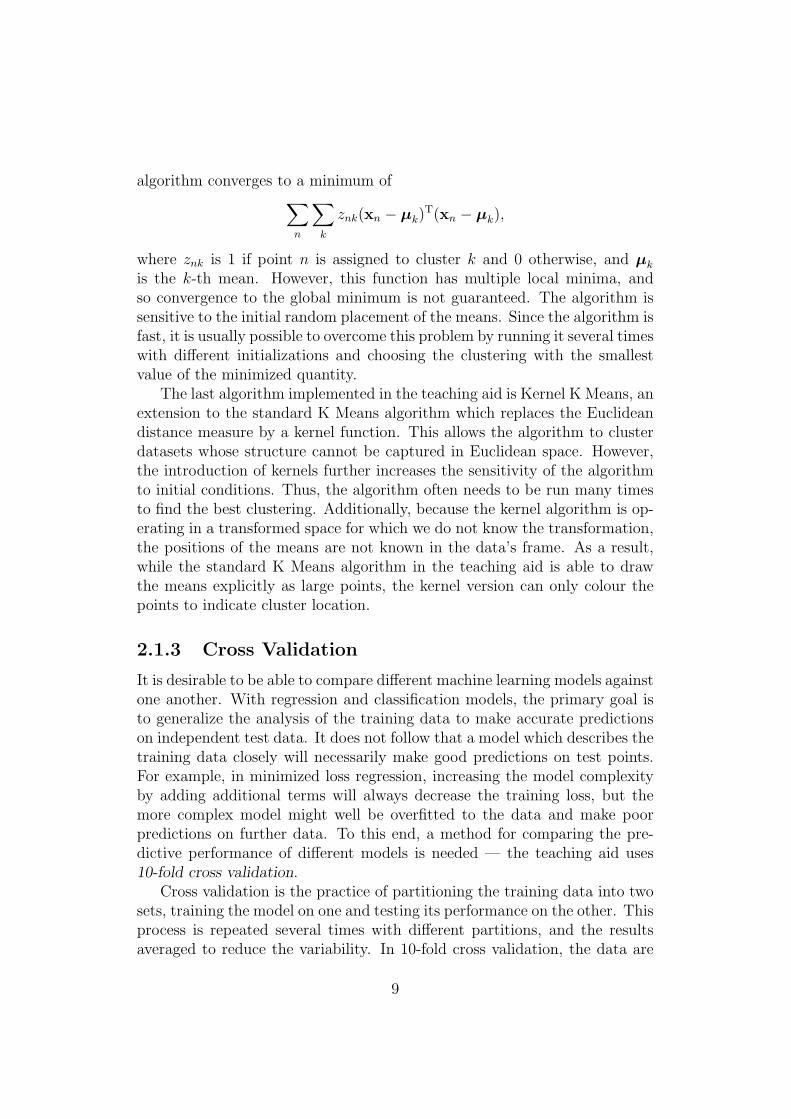
is the k-th mean. However, this function has multiple local minima, andso convergence to the global minimum is not guaranteed. The algorithm issensitive to the initial random placement of the means. Since the algorithm isfast, it is usually possible to overcome this problem by running it several timeswith different initializations and choosing the clustering with the smallestvalue of the minimized quantity.
The last algorithm implemented in the teaching aid is Kernel K Means, anextension to the standard K Means algorithm which replaces the Euclideandistance measure by a kernel function. This allows the algorithm to clusterdatasets whose structure cannot be captured in Euclidean space. However,the introduction of kernels further increases the sensitivity of the algorithmto initial conditions. Thus, the algorithm often needs to be run many timesto find the best clustering. Additionally, because the kernel algorithm is op-erating in a transformed space for which we do not know the transformation,the positions of the means are not known in the data’s frame. As a result,while the standard K Means algorithm in the teaching aid is able to drawthe means explicitly as large points, the kernel version can only colour thepoints to indicate cluster location.
2.1.3 Cross Validation
It is desirable to be able to compare different machine learning models againstone another. With regression and classification models, the primary goal isto generalize the analysis of the training data to make accurate predictionson independent test data. It does not follow that a model which describes thetraining data closely will necessarily make good predictions on test points.For example, in minimized loss regression, increasing the model complexityby adding additional terms will always decrease the training loss, but themore complex model might well be overfitted to the data and make poorpredictions on further data. To this end, a method for comparing the pre-dictive performance of different models is needed — the teaching aid uses10-fold cross validation.
Cross validation is the practice of partitioning the training data into twosets, training the model on one and testing its performance on the other. Thisprocess is repeated several times with different partitions, and the resultsaveraged to reduce the variability. In 10-fold cross validation, the data are
9

split into 10 folds of roughly equal size. The algorithm is trained on 9 ofthese folds, and the predictive performance on the held out fold is recorded.This is repeated 10 times, holding out a different fold each time, and thepredictive performance is averaged across the 10 rounds. The performancemeasure used is algorithm dependent — the testing loss for the minimizedloss method, test set likelihood for the maximum likelihood, and the numberof misclassifications on the test set for the classifiers. The teaching aid carriesthis process out and displays the averaged performance when the appropriatebutton is pressed.
Cross validation for clustering algorithms is not included in the applica-tion, since performance measures for clustering are application- rather thanalgorithm-specific.
10

Chapter 3
Survey of Related Software
To the best of the author’s knowledge, there is no existing software whichacts as an effective machine learning teaching aid across a variety of concepts.However, as part of the preparation for the development of the teaching aid, avariety of software products which accomplish some similar functionality werestudied. Additionally, several software libraries were considered for inclusionin the application in order to ease the implementation of certain features. Ananalysis of the strengths and weaknesses of these products follows, togetherwith a description of any influence they had on the final teaching aid.
3.1 Machine Learning Applets
There are a number of interesting Java applets freely available online whichillustrate machine learning concepts. [8] provides implementations of a vari-ety of algorithms.
3.1.1 Regression
Firstly, the author provides a simple least squares applet for linear regression.This allows the user to plot points by clicking on the applet, and it drawsthe best fitting straight line. The line updates each time a new point isadded. This ability to directly add new points is a highly useful one sharedby the other applets in the series, and this feature was incorporated into theteaching aid.
A second applet extends the functionality of the first by additionallyplotting polynomials up to fifth order for the data the user adds. This isimplemented rather poorly, however. It plots all five polynomials simulta-neously, and thus it is very difficult to distinguish between them. This is
11
worsened by the fact that all the curves are drawn in the same colour. Theteaching aid improves on this in its regression algorithms — the user is ableto add an arbitrary number of models, the terms for which are controlledindependently. For each model added, the colour can be chosen from a selec-tion of four. This allows more meaningful information to be extracted fromthe plot.
3.1.2 Classification
Also provided are a number of applets for classification, including one im-plementing the K-nearest neighbours algorithm. This allows the user to plottwo types of point (crosses and circles), then shades the background to showthe boundary between the two classes. The evolution of this decision bound-ary is intuitively clear as new points are added. However, the applet onlyimplements the algorithm for the case K = 1, which is a significant drawback.
The shading feature as a means of communicating the output of the clas-sifier is a very useful one, and was adopted as part of the teaching aid.However, the KNN implementation in the final application is significantlymore robust than the one in this applet. It allows choice between five classesrather than two, and the value of K can be set to any natural number. Thisallows the benefits and drawbacks of the algorithm to be more fully explored.
3.1.3 Clustering
Lastly, the applet suite provides an implementation of the K-means clusteringalgorithm. Users are able to plot points, and the applet assigns them to thenearest cluster and colours the background to show the current shape ofthe clusters. It is a reasonably clear implementation, but suffers from thelimitation that the number of clusters is fixed at four. Also, since the displayis updated after each new point is added, the clustering is initially veryunstable. This is somewhat visually confusing to an inexperienced user, andis not explained by the notes accompanying the applet.
Though a shading approach was found to be desirable for classification,for clustering it is less useful. In the teaching aid, the clusters are indicatedby recolouring the points to the same colour as their means. Additionally,any number of clusters can be specified, not just four. This allows differentclusterings to be compared against one another.
12

3.1.4 Discussion
A weakness of these applets in general is that there is no documentationbeyond a brief set of instructions for each. They assume some knowledgeof the algorithms they implement, which is a particular problem for theK-means applet. A novice to the subject would most likely be unable totake something meaningful from the symbols and colouring it uses. Moredocumentation would make a significant improvement to its usefulness. Thisillustrated a need for a help system in the teaching aid, which is included inthe final product. A collection of help files documenting each algorithm andfeature of the application can be accessed at any time while using it.
The applets do have a number of positive features. First, the source codeis freely available for inspection, and is fairly well documented and designed.This was instructive in the use of Java to implement machine learning al-gorithms. The code was studied during the proposal phase of the product,including the matrix implementation by the author. Though this was a use-ful introduction, ultimately the code for the teaching aid took few ideas fromthe applets. For one, the matrix implementation was not complete enough toeasily perform all the required operations, such as Cholesky decompositions.Additionally, the drawbacks of the algorithm implementations were deemedtoo significant to attempt adapting the implementations for use in the finalproduct.
The implementation as applets is also useful in that the software can bedistributed online very easily, and no installation or configuration is requiredby users. The possibility of adapting the teaching aid into an applet wasexplored during the development, but was ultimately discarded due to timeconstraints. An adaptation of the software into an applet, or to run usingJava’s Web Start system, represents useful future work.
3.1.5 Gaussian Processes
Another machine learning applet is detailed in [9], which covers Gaussianprocesses. This is a more polished product than the other applets whichhave been discussed. It allows the user to plot some points, choose a type ofcovariance function, and choose the parameters of that function. The appletthen draws the mean curve together with an indication of the variance. Thesoftware is supported by useful documentation and plentiful links to otherinformation on the subject. However, the applet itself tends to be slow inresponding to user input. Since the source is not available, the reason forthis is not clear.
Gaussian Processes were not included in the teaching aid as there was
13

insufficient time to implement the algorithm. As quite a complex technique,it was deemed too risky to implement, particularly since the algorithm isnot covered in the current machine learning course. Nonetheless, addingfunctionality similar to that found in this applet would be a useful additionin the future.
3.2 Weka and Java-ML
There are a number of Java libraries which implement machine learning algo-rithms. Two of the most prominent are Weka [12] and Java-ML [1]. Both areopen source projects which provide powerful and robust implementations ofa wide variety of algorithms. The code is well designed and extensively doc-umented, and thus can provide insight into writing efficient machine learningprograms. However, both are designed to be used on real world data sets andas such provide implementations which are more complicated than strictlynecessary for the scope of this project. Their use was considered for assis-tance with the project implementation, but ultimately it was decided thatthe libraries would add significant ‘bloat’ to the application and the cost ofintegrating them with the desired functionality was too high.
3.3 MATLAB and Octave
3.3.1 MATLAB
MATLAB [16] is a powerful numerical computing application, and also thename of the scripting language used by that application. It is the currentstandard for lab use in the machine learning course, as well as enjoying wides-pead popularity in the academic and industrial communities. It provides so-phisticated functionality for manipulating matrices and plotting data, whichmay be used to implement and visualize a wide variety of machine learningalgorithms. However, despite this power, it is far from an ideal environmentfor the purpose of teaching inference ideas. While it is possible to gener-ate data using MATLAB, it is far from intuitive for a novice user to doso, and similarly algorithm implementation can be tricky. There is a signif-icant learning overhead associated with mastering the MATLAB scriptinglanguage which is often a hindrance in the course lab sessions. Indeed, inorder to make progress on some of the more difficult algorithms, students areprovided with implementations and left to observe the effect of altering theparameters. Even this is not simple – parameters must be changed in textfiles and the script must be re-executed after each change to see the effect.
14

This disconnect renders the system unintuitive for illustrating the algorithmconcepts. The teaching aid application provides a continuous interactionstyle which is far more intuitive to use.
3.3.2 Octave
Another main drawback of MATLAB as a teaching tool is its cost. Thesoftware is proprietary, and individual licences for the software are very ex-pensive, and as such it is unlikely a student will be able to afford one. Thus,students cannot install the software on personal machines and are limitedto using MATLAB within the departmental labs. This is somewhat imprac-tical, particularly during revision periods when students are not normallyon campus. However, this problem is partially solved by the existence ofGNU Octave [19], a free and open source numerical computing environmentwhich is largely interoperable with MATLAB. Distributions of the softwareare available for Windows, Mac and most prominent Unix-like operating sys-tems. Hence students can readily obtain a copy to experiment with at home.It shares many benefits with MATLAB, but also suffers from the same draw-backs for use as a teaching aid. Additionally, it uses a command line interfacewhich is less intuitive than the MATLAB GUI. Octave’s plotting capabilitiesare also slightly less powerful, utilising the open source gnuplot program.
3.3.3 JavaOctave
JavaOctave [13] is a software module which allows Octave calculations to beperformed from inside a Java application. Its use as part of the teaching aidapplication was initially considered, since it would potentially simplify algo-rithm implementation by allowing reuse of scripts that were written as partof the machine learning course. However, this would restrict the applicationto use on systems where Octave was installed and it was decided that thiswas a poor design choice. JavaOctave was also considered for use as part ofthe development process, using calls to Octave to check the correctness ofthe Java algorithm implementations. However, some initial experiments withthe software were not promising. Its syntax is quite unwieldy, and it proveddifficult to perform even simple calculations without running into frequenterror uninformative error messages. Ultimately it was decided that the costof learning the syntax and integrating the testing with the teaching aid wouldbe too high, and would produce only limited benefit. The use of the softwarewas thus deemed unviable.
15

3.4 Mathematics and Statistics Libraries
Much of the code for the teaching aid application involves determination ofparameters by performing operations on vectors and matrices, and the Javaclass libraries do not have support for these. In order to avoid writing codeto perform basic matrix operations, which would take some time to do com-prehensively, a number of software libraries implementing this functionalitywere considered.
3.4.1 Apache Commons Math
Commons Math [2] is a library produced by the Apache Software Foundationwhich provides a number of mathematical and statistical features not avail-able in the Java platform. In particular, it provides linear algebra packageswhich enable matrix operations and the solution of systems of equations.The library also has features for random data generation in a variety of for-mats and for statistical functions including least squares regression. Thesefeatures were certainly desirable, but the library also includes a large amountof functionality which is outwith the scope of the project. For example, it hasclasses for solving ordinary differential equations and implementing complexnumbers. In total there are over 30 packages in the library, with the sourcecode occupying around 6MB.
An additional point is that the code in the library is designed to be verygeneral, and using it as part of the teaching aid would have required datato be stored in generic structures which are more complex than necessaryfor the purposes of the application. This would have added a further costto integrating the library, detracting from useful development time. As withJavaML and Weka, the library was ultimately decided to be too bloated andcomplex for inclusion in the teaching aid code.
3.4.2 JAMA
JAMA [17] is a linear algebra package for Java, developed by the Mathworksand NIST. It provides operations for constructing and manipulating realmatrices, together with functionality for solution of systems of equations andseveral common matrix decompositions. The implementation is compact,using only six classes in a single package, and the primary data structure is asingle Matrix class. It provided sufficient operations to implement all of thealgorithms in the teaching aid, and given its size was easy to integrate withthe rest of the application. Further, the classes are well designed, readableand suitably commented, so that the implementation is easy to understand.
16

This made use of the library very simple. Hence, JAMA was used in theapplication to accomplish the required mathematical functionality.
3.5 Quadratic Programming
As discussed earlier in this document, one of the more complex algorithmsin the teaching aid is the Support Vector Machine. The complexity arisesover the solution of a quadratic programming (QP) problem as part of thealgorithm. Ultimately, this problem was overcome by implementing Platt’sSMO algorithm as an alternative to a direct QP solution. However, theauthor did not discover SMO until later on in the development process. Priorto this, a number of options were considered to act as a QP solver for theteaching aid.
3.5.1 LibSVM
LibSVM [4] is a software library for support vector classification in general.It provides implementations of the basic SVM classifier, as well as extensionsfor regression and distribution estimation. It also supports a multi-classextension of the SVM technique. Implementations are available in a variety oflanguages, including Java. However, there were a number of reasons to avoidusing the library in the teaching aid. Firstly, the extensions it incorporatesare well beyond the scope of the project. Secondly, the Java implementationprovided is poorly laid out and difficult to read. Much of the code is organizedin a single file which contains multiple inner classes and few comments. Thealgorithms used are not described well (if at all), and the time necessaryto gain an understanding of the code and integrate it with the teaching aidwould have been infeasibly long.
3.5.2 QuadProjJ
QuadProgJ [23] is a Java solver for strictly convex quadratic programmingproblems. It implements the dual active-set algorithm developed by Gold-farb and Idnani [11]. The code is clearly commented and easy to understand,and is contained in a single class. It was a potential candidate for use dur-ing the project, but was ultimately rejected for a number of reasons. Forone, it uses a matrix implementation from Colt [3], a mathematics librarydeveloped at CERN which is similar in many ways to Commons Math andso was too complex for the needs of the application. If QuadProjJ were tobe used, its implentation would have needed to be adapted to use JAMA
17

matrices. This would likely have been possible within the time allowed forthe project. However, a second concern is that the code takes in the QPproblem framed in a slightly different format to that required for the SVM,and so a certain amount of preprocessing would have been necessary withinthe teaching aid application. The combination of these factors led to thedecision that integrating QuadProjJ with the teaching aid was too expensivein terms of development time.
3.5.3 New Implementation
The other option which saw serious consideration was to write an entirely newQP solver. The obvious advantage was that this provided freedom to choosethe format to match the needs of the SVM algorithm. Chapter 12 of [14]provides an extensive guide to implementing a quadratic programming solverin Java, and would have been used as a basis for the code in the teaching aid.However, the SMO algorithm was encountered, and is considerably easier toimplement than a QP solver, rendering this decision moot.
3.6 Plotting
Obviously, a significant part of the teaching aid application is its ability toplot data points and curves. A number of Java libraries were considered toassist this aspect of the functionality. These included JFreeChart [18] and theScientific Graphics Toolkit (SGT) [7]. These, and other libraries like them,provide support for creating graphics in a variety of sophisticated ways. Forexample, many libraries allow time series plots, bar charts and histogramsto be generated. Most of this functionality is redundant for the needs of theproject – the teaching aid is primarily concerned with simple XY plots andwith colouring the display based on a grid. The library which comes closestto matching these requirements is the SGT, but even that provides morethan is needed.
It was therefore decided that the required plotting tools could most easilybe implemented using the core classes provided in the Java Swing library.The plotting is all handled by a custom class which extends Java’s JPanel.
18

Chapter 4
Requirements
4.1 Requirements Capture Process
From the outset, the project had a well defined aim: design and implementan application to teach some fundamental machine learning concepts. Theearliest part of the development process was to refine this overarching aiminto a basic set of requirements from which to build the application. Theprimary stakeholder in the project is Dr Simon Rogers, as both the projectsupervisor and a likely future user of the software. The largest part of therequirements gathering process took the form of a series of meetings withhim, discussing the features that were desirable. This led to an initial list ofrequirements, prioritised according to the MoSCoW method. [5]
Additionally, the survey of related software highlighted a number of usefulfeatures which were not initially considered by the client. This was anothersource of refinements to the requirements document. In particular, the abilityto add single points by clicking was not an initial requirement, but was addedto the list after it was encountered in another piece of software.
The final part of the requirements gathering process was an email sentto the students undertaking the machine learning course in the 2009/2010session. The students, as potential users of a teaching aid, were asked toidentify features they would find useful in such an application. Only a smallnumber of responses were obtained, which did not add any entirely newrequirements. The value in these responses came in identifying which algo-rithms were most conceptually challenging, and hence should be prioritisedin the implementation.
A brief overview of the requirements obtained now follows. The full listof requirements and a list of derived use cases are included in appendix Aof this document. However, it should be noted that some of these are left
19

purposefully general. This decision was taken in order to allow flexibility ofthe precise details if any difficulties became apparent during the developmentprocess. Indeed, the formal requirements capture phase of the project wasrelatively short. This was in keeping with the chosen development model,an agile process which attempted to avoid excessive heavyweight design andfocus instead on short, frequent iterations of design and implementation.
4.2 Requirements Overview
Starting from the basic aim of the project, two fundamental requirementswere immediately obvious. First, it must be possible to generate data, andsecondly it must be possible to run an algorithm on that data. These basicgoals were then broken down into more detailed requirements. For example,the ability to add and remove single points directly, and to sample multi-ple points from a given distribution, were added as extensions of the datageneration requirement.
A less critical, though still highly desirable, set of requirements arosearound the storage of data. To enable interesting cases to be easily demon-strated, a requirement for the saving and loading of datasets was added. Ad-ditionally, the project supervisor requested that the facility to export imagesof the plot be added. This was added as “could have” under the MoSCoWsystem, as the teaching aid could easily be deemed functional without it.
A small number of non-functional requirements were also identified. Fore-most among these was that the teaching aid should be developed in Java, toallow for easy deployment over a variety of platforms. Also, the GUI shouldbe designed with users who have a basic grasp of machine learning terminol-ogy in mind. Nonetheless, it should be designed to be as usable as possibleeven for novice users. Finally, algorithm implementations should be made asefficient as possible in order to account for the possibility of large trainingsets.
20

Chapter 5
Analysis and Design
The next step in the development was to analyse the requirements and prob-lem domain to identify a class structure for the teaching aid’s core features.Individual algorithms were not designed in detail before the implementa-tion began. Rather, a basic framework for the model was created, coveringalgorithms and data. Alongside this, a design for the key elements of thegraphical user interface (GUI) was produced.
The overall design attempted to follow a Model View Controller architec-ture [21] — the Model is represented by the algorithm implementations, andthe View by the plotting functionality present in the GUI. There are no pureController classes, however. Instead, each algorithm has an associated classwhich handles both the user interface aspects of setting options for the algo-rithm, and the logic of training the algorithm and addings its output to thedisplay. Thus, these classes fall somewhere between the View and Controllerroles.
A more detailed treatment of the design now follows.
5.1 The Domain Model
The domain model of the teaching aid is the part of the system which de-scribes the machine learning entities and the relationships between them.From studying the requirements, it was immediately clear that two of theimportant objects to model were algorithms and data points. Each of thesewas chosen as a candidate class. Additionally, it was clear that a collectionclass for data points would be necessary — this became the Dataset class.These three classes formed the basis for the two core domain model packages,algorithms and data.
21

5.1.1 The data Package
Datapoints
The Datapoint class represents a single point. Each point is modelled by itslocation in two dimensional space together with a label. This is not entirelyaccurate to the underlying machine learning model for all algorithms. Forexample, in regression a point is defined by only its x coordinate and itslabel t. However, given that all plots produced by the teaching aid are intwo dimensions it seemed a good idea to have the data kept in this stan-dard structure across all algorithms. Though those two dimensions representdifferent quantities for different families of algorithm, this implementationdecision is unseen from a user’s perspective, and using a standard formatmakes algorithm implementation easier.
The initial Datapoint design included a number of other features. First,each point can have an associated error bar, represented by a boolean variableindicating whether or not to draw the bar and a double representing thesize of the error. This was added to allow regression algorithms with ameasure of predictive uncertainty to show this uncertainty when the outputis drawn. Secondly, each point also holds a boolean indicating whether thepoint is to be highlighted when drawn. This was added with the intentionof visually showing which points are support vectors for the SVM algorithm,but algorithms added in the future could also conceivably highlight points,hence why the feature was added to the Datapoint class rather than to theSVM algorithm itself.
Useful methods in the class include one to determine whether a point‘contains’ an (x, y) pair or not. This allows the teaching aid to determinewhen a point has been clicked on. Also, a method was added to determine theEuclidean distance of the point from a second point passed as a parameter.This is useful for a variety of other features in the teaching aid, such asfinding the neighbours in the KNN algorithm.
Datasets
As well as operations on single points, it is important for the teaching aid tobe able to operate on collections of points. The Dataset class controls thisfunctionality. It maintains a collection of Datapoint objects, implementedas a list since the order of points can be important — for example, wheninterpolating between points to draw a line. An integer field called style
is also maintained, which describes how the dataset should be drawn. Op-tions include discrete points, interpolation in order between the points, andshading. This field is accessed by the GUI when a dataset is plotted.
22

The majority of methods in the class are for adding, removing and access-ing points. Additionally, there are two noteworthy methods which should bementioned. The first is kNearest, which takes a Datapoint and an integer kas parameters and returns a Dataset object containing the k nearest pointsin the set. This is clearly useful for implementing the KNN algorithm, andkeeps the internal representation of a Dataset hidden from client code. Thesecond important method is fold. This takes an integer n as a parameterand returns an array of n Dataset objects, each containing approximately ann-th of the points in the dataset. The partitioning of points between foldsis random. This method is intended to simplify the implementation of crossvalidation.
Sampling
One of the requirements is the ability to sample data from a given distribu-tion. At this stage of the design, methods for doing this were not studied ingreat detail. However, in order to facilitate this at a later stage, an abstractclass Sampler was added to the data package. This specifies an abstractmethod, nextPoint, which returns a Datapoint. Individual samplers cansupply an implementation of this method, which can the be called by theGUI as many times as necessary to generate the required data.
5.1.2 The algorithms Package
The Algorithm Class
The primary class in this package is Algorithm. This is an abstract classwhich defines the core methods any algorithm must implement. It also definestwo fields which all algorithms require — one is the training data, a Datasetobject, and the other is a boolean variable indicating whether the output ofthe algorithm should be drawn or not.
The two most important methods in Algorithm are train and predict.The former takes in a Dataset object and trains the algorithm on the pointsin the set. The latter takes a Datapoint and returns the numerical output ofthe algorithm on that point. These methods represent the two fundamentalmachine learning operations that the teaching aid performs.
The Algorithm class also specifies an abstract method getOutput whichis used to obtain an algorithm’s output for plotting. This method takes aDataset as a parameter, and returns another Dataset with the appropriatestyle and values for plotting. The type of Dataset passed in and out dependson the particular type of algorithm. For example, a regression algorithm is
23

only concerned about the x values of the points in the input set, and returnsa set of (x, y) pairs which can be interpolated to draw a curve. A classifier,on the other hand, takes a grid of points as an input and returns the samegrid, but with the points coloured according to the output of the classifier.This distinction led to the introduction of a further set of abstract classesinto the design.
Abstract Subclasses
The logic of plotting an algorithm’s output varies between the different fam-ilies of algorithm — classifiers, clusterers and regression techniques — butdoes not vary inside those families. For example, KNN and SVM both pro-duce a coloured grid as their output. Thus, a second level of abstraction wasadded to the design. Rather than have individual algorithms extend the Al-gorithm class directly, three intermediary classes were identified. These arethe RegressionAlgorithm, Clusterer and Classifier classes. Each of these ex-tends Algorithm with some new features specific to their family of methods,but all three classes are still abstract. The actual algorithms in the teachingaid all extend on of these classes.
There are a number of advantages to this design. First, it enables the useof the heterogeneous list pattern. When training an algorithm, the teachingaid need not know the specific technique it is training, and can instead callthe train method from Algorithm. On the other hand, the additional layerof abstract classes allows enough flexibility to plot the different types ofalgorithm, but is not so vague that each algorithm requires its own plottingcode. This simplifies the GUI implementation.
The RegressionAlgorithm class adds a number of features to the basicAlgorithm class. It defines eleven integer constants representing the functionsh(x) which the teaching aid recognises as valid terms in a regression problem.The integers 0–8 represent polynomial terms from x0 up to x8, 9 representssinx and 10 is ex. Whether or not a given term is used by the algorithmis governed by a boolean array terms of length eleven. If the i-th entryof this array is true, then the function corresponding to the class constanti is included in the regression. For example, if terms[0], terms[3] andterms[9] are true and the remaining entries are false, the algorithm will fita model of the form w0 + w1x
3 + w2 sinx. This design has the advantagethat it is easily extensible through the addition of new class constants fornew functions and an increase in the length of the array.
This class also contains a variant of the getOutput method which takesan array of doubles representing the x coordinates rather than a Dataset asits input. While this variant is not strictly necessary it is a useful convenience
24

method — computing the output values is faster since the input does notneed to be wrapped in a Dataset.
Other fields introduced in this class include three Matrix objects namedX, t and parameters. These correspond to the matrix X and the vectorst and w as defined in section 2.1.1. The notation for these quantities isstandard across a wide variety of linear regression techniques, so it seemsobvious to include them as instance variables.
The class Classifier adds no new fields to the basic Algorithm structure.It does, however, add two new methods. One is classificationErrors,which takes a Dataset and returns the number of misclassifications the al-gorithm makes on the data. A misclassification occurs when the algorithm’sprediction for the label on an (x1, x2) pair does not match the actual label onthe point. To make this simpler at the implementation stage, a second newmethod, predictLabel, was added. This abstract method forces a classifierto assign a label to a Datapoint. For some algorithms, such as KNN, this willreturn the same result as the basic predict method, but for others the twomethods will return different numbers. For example, predict for an SVMwill return some real value on a given point, and predictLabel will assign alabel to the point based on the sign of that prediction. The decision to im-plement predictLabel as a separate method was taken to reduce repetitionin the design. The abstraction of the label assignment means the misclassi-fication count can be implemented at the Classifier level, rather than havingseparate methods in each class which extends Classifier.
The Clusterer class adds no new instance variables or methods. Its onlypurpose is to allow algorithms to be referenced as clusterers by the GUI,without needing to know the specific algorithm.
Specific Algorithms
Individual algorithms were not designed in detail at this phase of the devel-opment. It was decided that the framework described above was a sufficientbasis from which to start the development process. Many algorithms canbe implemented fully using only the abstract methods defined in the frame-work. Some, particularly the clusterers, were later found to require additionalmethods specific to each algorithm. However, the risk posed by designing andimplementing those methods as they were encountered in the developmentprocess was deemed very low.
A final detail added to the design of the domain model was to add threesubpackages to the algorithms package, one for each of the main algorithmfamilies. This makes the structure of the domain clearer, and groups logicallyrelated classes together. A class diagram for the domain model as of the
25

completion of the project is shown in figure 5.1.
Figure 5.1: Domain Model Class Diagram
5.2 Graphical User Interface Design
As discussed in section 3.6, the proposal phase of the project identified thatthe optimal method to implement the teaching aid’s GUI was to make use ofJava’s Swing framework. This toolkit, a core Java component contained inthe javax.swing package, provides lightweight implementations of a varietyof GUI components such as buttons, panels, tables and trees. It provides anumber of flexible layout managers for controlling the appearance of an ap-plication, and combined with the java.awt.event package offers support forfiring and handling a variety of events. It is also simple to implement a customcomponent by extending a Swing class and overriding its paintComponent
method.
26

5.2.1 Basic Layout
The first step in designing the GUI was to identify the key information theinterface had to communicate, and to determine a possible layout for thisinformation. The important information identified was:
• The available algorithms, and the one currently selected
• Any options for configuring the selected algorithm
• Options for generating data
• Most importantly, the plot of the data and the algorithm output
The next step was to draw up a mock interface showing a possible layoutfor these four items. A simple drawing of the proposed layout is shown infigure 5.2. This is very close to the final layout of the program. A slightlyearlier version of the design had data generation as an additional option onthe list of algorithms, but on further reflection this was a poor idea. Forone thing, the number of classes allowed varies by algorithm, so a singleindependent data generation feature would work poorly. Additionally, it isuseful to be able to add new data after an initial model has been trained.Thus, the second version of the design includes an explicit area for datageneration options.
Having identified this layout, a more detailed GUI design was produced,specifying a class structure and identifying which Swing components wouldbe used to implement particular sections. The classes were not designed inprecise detail at this stage — the buttons, drop down menus and so on forspecific options were left to be added at implementation time. It was moreimportant to capture the main interface classes and the relationships betweenthem.
To prevent any one class from becoming too complex, the various parts ofthe functionality listed above were given their own class. The first of these isAlgorithmPanel, a class which handles algorithm selection. Swing providesa number of widgets which implement selection from a set of options. Thetwo most appropriate components are JList, which simply displays a list ofelements and allows mouse selection of the entries, and JTree, which displaysa hierarchically ordered list. The latter was chosen because the tree allowsthe models to be clearly grouped together by type. The class AlgorithmPanelextends Swing’s JPanel, a generic container class, and has a JTree field toshow the algorithms.
Data generation is handled by the class DataPanel, which also extendsJPanel. This class displays its options in two subpanels. The first controls
27

Figure 5.2: A basic interface mockup, showing the core features
the settings for the points to be added — a set of radio buttons for choosingbetween the training and test data sets, a button to remove all points fromthe display, and a drop down menu to choose the class. The last of theseonly appears for classifiers, and the number of classes available varies asappropriate for the selected algorithm.
The other subpanel in Datapanel provides the options for data genera-tion. At the design stage, the full range of generation techniques was notwell defined. The initial suggestion from the project supervisor was to addpolynomial sampling. Thus, the instance variables added at this stage weretwo drop down menus (JComboBox) to select the polynomial order and anominal value for the noise. Additionally, a text field to specify the numberof points and a button to generate the data were added to the class design.Other types of data generation and their associated widgets were added tothe class as neessary during the implementation phase.
The interface as a whole is controlled by the class MainGUI. This extendsSwing’s JFrame, a heavyweight class which implements a window to containall the other GUI elements. The main responsibility of this class is to createand layout the other panels. Additionally, it has a JMenuBar to control theapplication settings which are not specific to any one algorithm. Anotherimportant responsibility of the class is to provide the logic for loading analgorithm. When the user selects a new algorithm from the tree, the con-
28

figuration panel for that algorithm has to be added to the display, and theappropriate data generation options enabled. Having AlgorithmPanel han-dles these tasks would introduce a high degree of interaction coupling intoits design and reduce the overall cohesion of the class. Thus, MainGUI hasa loadAlgorithm method which accomplishes this setup process. This is acleaner design, reducing the degree to which the GUI’s component classesneed reference one another.
5.2.2 Plotting
The central goal of the teaching aid is the visualization of machine learningalgorithms, and so the plotting functionality is the most important area ofthe application. The design delegates all plotting tasks to the class Plotter,another JPanel extension. Having the semantics of plotting separate fromthe algorithm implementation increases the cohesion of the design, in that analgorithm is only concerned with machine learning problems and need not beconcerned with how its output is drawn. This offers a further advantage inthat the plotting mechanism can be altered in the future without requiringchanges to the underlying algorithms.
The important fields in Plotter include a Set of Algorithm objects, aHashMap relating double values to colours, and two Datasets — one forthe training data, and one for the test data. Maintaining a collection ofAlgorithms allows multiple models to be drawn at the same time, a usefulfeature for regression methods. The mapping of doubles to colours allows thelabel on a Datapoint to be used to determine its colour when it is drawn. Thepresence of a separate test Dataset allows the performance of a model to beevaluated independently of its training set, an important feature since goodtest predictions are the goal of the majority of machine learning techniques.
Plotter is the largest class in the teaching aid, and this was the casefrom the design stage onwards. The central method is plot, which takes aDataset and draws its output on the screen. The same method is used forplotting the training and test sets, and for plotting the set returned by eachalgorithm’s getOutput method. Different types of dataset — points, curvesand shaded grids — are distinguished by their style field. A supplementarymethod, plotErrorBar is included to draw the error bars for any pointswhich are flagged to show them. There is also a method to draw the axeson the plot. These three methods were designed to be called from withinPlotter’s paintComponent method, which guarantees that all changes to thedisplay are made in a thread safe manner.
Plotter also has methods for converting back and forth between the coor-dinate system used by the physical panel and the data’s frame of reference.
29

Swing components have an internal coordinate system which places the ori-gin at the top left corner and marks coordinates in integer steps, with thex coordinate increasing to the right and the y coordinate increasing down-wards. This results in many points having large values, which can makematrix inversion more computationally intensive, a potential problem for re-gression algorithms in particular. As a result, the coordinates of the dataare transformed into the range [−10, 10] × [−10, 10] for storage. The inte-ger coordinates are recovered through an inverse transformation when pointsneed to be drawn. This design has the additional advantage that resizing thedisplay is very simple, since the height and width of the panel can be useddynamically in the transformation.
The final important feature of Plotter is that it implements the MouseLis-tener interface specified by java.awt.event, allowing the panel to listen formouse clicks on itself. The class has a number of methods which can becalled to add and remove Datapoints when the user clicks on the plot.
5.2.3 The OptionPanel Class
Each algorithm in the teaching aid has its own particular set of configurationoptions, so an all purpose class to manage the interface for these would bea poor idea. At best such a class would be visually crowded and confusing,and in all likelihood would be unusable. From a design and implementationstandpoint, a generic options class would have poor cohesion and would bedifficult to maintain and extend. Clearly, a stronger design is necessary.
To this end, the teaching aid has the OptionPanel class. This is a verysimple JPanel extension which acts as a placeholder for the right hand part ofthe display when no algorithm is loaded. It specifies a single instance variable,an Algorithm. The options for each individual algorithm are controlled bya class extending OptionPanel. The base class specifies a protected methodlayoutPanel which adds the introductory text to the panel, but subclassescan override this method to layout the GUI elements they require. This de-sign allows as much customization as needed, but does not require the restof the GUI to know about each of the different subclasses. In particular,MainGUI maintains an instance variable of type OptionPanel as part of thelayout, but this can be set to any of the specific subclasses by calling theappropriate constructor in MainGUI’s loadAlgorithm. This is a simple de-sign, but is still flexible and easily extendable. The class OptionPanel andits subclasses make up the gui.data subpackage.
30
5.3 Modularity
From the outset of the project, one of the design features which was deemedmost important was modularity. This refers to the ability of the teachingaid to be easily extended to incorporate new algorithms. The motivation forthis was twofold. First, designing to ensure modularity encourages focused,cohesive classes and a clear separation between the interface and the under-lying models. Secondly, if another developer wishes to extend the teachingaid in the future by adding new algorithms, a modular design clearly makestheir task simpler.
The decision to keep plotting and algorithms separate means that de-velopers can add new algorithms without altering the existing Plotter class.They need only implement their algorithm along with an OptionPanel sub-class to control its settings. The steps necessary to add a new algorithm aidare as follows:
1. Write a class to implement the algorithm, extending either Classifier,RegressionAlgorithm or Clusterer
2. Write a control class for the algorithm, extending OptionPanel
3. Add the name of the algorithm to the JTree in the AlgorithmPanelclass (1 line of code)
4. Add code to loadAlgorithm in MainGUI to handle the specifics ofloading your algorithm (∼ 4 lines of code)
Clearly, the process is a simple one. Excluding any difficulties inherent inimplementing the algorithm, very little effort is required to integrate the newalgorithm with the teaching aid.
5.4 Final Design
During the implementation process, a number of other packages and classeswere added to the teaching aid over and above those which were designedinitially. The final package diagram, along with class diagrams for each pack-age, are included in appendix B of this document. The interesting featuresof some of the additional classes are discussed at greater length in the nextchapter. For the classes discussed in this chapter, the final designs reflectmore methods and instance variables than were mentioned in the discussion.These represent routine implementation details which were not interestingenough to discuss in detail here, and added nothing novel to the design. A
31

description of the purpose of each of the variables and methods in the teach-ing aid is available in the automatically generated Javadoc, which may befound on the accompanying CD.
32

Chapter 6
Implementation
With a strong design in place, the next phase of the project was to implementthe teaching aid. This chapter gives an overview of the implementationprocess, and describes in detail some of the interesting difficulties whicharose during the development, and the corresponding solutions.
The application was written in Java, using the Eclipse IDE. It was builtand tested primarily using version 1.6.0 of Java, running on Microsoft Win-dows Vista. Some additional testing was carried out in Ubuntu Linux, andthe weekly demonstrations of the teaching aid to the project supervisor usedApple’s OSX. Thus the application saw use on a variety of platforms and thecore functionality worked as expected on all of them.
6.1 Development Method
The initial project proposal called for the development to be carried out ac-cording to the Feature Driven Development (FDD) [6] model, which involvessuccessive iterations of design, implementation and testing to produce smallmodules of code called features. This was chosen because it seemed to fitwell with the desired modular nature of the project — each algorithm isessentially a feature.
However, due to the time constraints involved in the project, it was de-cided that the FDD model was too granular in its definition of developmentphases. It places emphasis on planning and designing on a per feature basis,then refining the overall design model before actually writing any code fora given feature. This seemed somewhat redundant in the case of the teach-ing aid, because care was taken in the initial design to ensure good use ofinheritance structures so that any one algorithm implementation should re-quire very little additional design. Therefore, the development model chosen
33

amounted to an agile development spin on the FDD model.Each new algorithm was briefly analysed to identify the additional meth-
ods, if any, which would be required to implement the algorithm. The algo-rithm was then immediately implemented, followed by its option controllerclass. The controller classes were designed with quick sketches identifyingthe buttons and other GUI elements which were necessary to control the cor-responding algorithm. Next, the controller was integrated with the GUI —by design, this was a very quick and easy process. Finally, the new algorithmwas tested to ensure its output was correct and there were no plotting errors.Once it was clear that the algorithm was working as intended, developmentmoved on to the next feature.
6.2 First Prototype
Before implementing any algorithms, the first step of the implementationprocess was to build the basic framework for the GUI. No interaction wasadded at this stage. Rather, the primary concern was to get the layoutcorrect and add the core GUI elements. This initial prototype correspondedto a basic implementation of the MainGUI, AlgorithmPanel, DataPanel andOptionPanel classes. Most of this process was straightforward and did notdeviate from the design. A screenshot of the application at the end of thisphase in the development is shown in figure 6.1.
In AlgorithmPanel, the tree showing the basic algorithm types is included,but at this stage the only explicit algorithm displayed is minimized loss. Thisis because the list of algorithms had not been finalized at this point in thedevelopment. Minimized loss was chosen as the first because it is a verysimple algorithm and would be easy to implement. The plan for addingmore algorithms was to implement one of each family as quickly as possible,then to add as many further algorithms as the development time allowed.
The OptionPanel class contains only a label inviting the user to choose analgorithm. Since no algorithms were coded, no child classes of OptionPanelwere added either. However, one useful feature that was added to the designat this part of the process was placing the options in a tab pane, representedas a JTabbedPane in the MainGUI class. This can be seen in the screenshotas the tab with “Welcome” written on it. This was added to allow for thepossibility of multiple simultaneous models for some algorithms. Each modelcan have its option panel in an individual tab. The other option consideredfor multiple models was to open successive option panels in small separateframes. This was rejected because it would add too much clutter to the screenand would make it too easy to lose a panel behind other windows. The tab
34

Figure 6.1: Early GUI Prototype
pane approach allows many models to be controlled using a small area ofscreen space, and makes switching between models clear and intuitive.
The version of Plotter implemented in the prototype was very basic. Itimplemented the MouseListener interface but did nothing in response to anyMouseEvents. The only things drawn by the paintComponent method werethe axes.
The DataPanel class has a number of its key features in place in the proto-type. The two subpanels are clearly identified and labelled. The ‘Points’ sub-panel has two JRadioButtons to choose between training and testing points,and a JButton to clear all points. The ‘Generate Data’ subpanel has a JCom-boBox to select the type of model to sample from, although no options wereadded to it until later. Finally, a JTextField to enter the number of pointsto sample and a JButton to carry out the sampling are included.
Note that no menu bar was added to the GUI for this prototype becausethe functions for the menu had not been clearly defined.
While most of the implementation up to this point was simple, a small
35

number of problems did occur. First, it was discovered that adding a JTreeobject directly to the AlgorithmPanel caused strange visual effects. Thewhite background of the panel shrunk to match the exact size of the tree,leaving large gaps of grey space which were visually unappealing. This prob-lem was solved by adding the JTree to a JScrollPane, and adding that paneto the panel as a whole. This kept the background at the full size of thepanel, as intended. This adds an additional benefit in that it allows scrollbars to be added in the event that the tree becomes too wide to be displayedin the allocated width.
A second problem was that laying out the component panels of the GUIwas not as simple as anticipated. Adding the component panels directlyto MainGUI was tried using a variety of Java’s available layout managers,but it was impossible to line up the components as desired and have themmaintain their relative positions as the frame was resized. An initial solutionconsidered was to fix the size of the window, but this is a suboptimal solutionas users with large screens should be able to increase the size of the teachingaid and gain a clearer view of the plot. The problem was eventually solvedthrough the introduction of a number of additional JPanels in MainGUI,which were used to contain the key GUI components and allow more precisecontrol over the layout. This makes the layout code fairly involved and addsa variety of instance variables which have little to do with the overall goalsof the teaching aid, but these side effects were unavoidable.
6.3 Adding Interaction
6.3.1 Datapoints and Datasets
Once the basic interface framework was ready, the next task was to addcore functionality by implementing the use cases. For this to happen, theDatapoint and Dataset classes had to be implemented. Datapoint is a verysimple class, and none of the methods caused any implementation difficulties.The same is largely true of Dataset, with the exception of the kNearest andfold methods. These required additional planning to implement successfully.
The algorithm created to split a dataset into folds is shown in 6.3.1.Essentially, the algorithm distributes the points in the dataset as evenlyas possible across the folds, then assigns any that are left over to randomfolds. The order in which points are chosen to be assigned to a fold israndom. All random numbers required for the algorithm are generated bythe Random class, a part of the core java.util package. An unexpectedbenefit of the decision to use a List to represent the contents of a dataset was
36

that implementing this algorithm in Java became very easy. Once the indexof the next point to be added to a fold was identified, the steps of removingthe index from the List indices and getting the corresponding Datapointcould be carried out in a single line of code.
An initial mistake made when implementing the algorithm was to passthe points from the main dataset to the folds by reference. Thus the samepoint was referenced by both Datasets, and the original could have the stateof its points changed when this was not intended. This could occur duringcross validation, for example. To solve this problem, the Datapoint class wasaltered to include a method clone which returns a new Datapoint object withthe same position and label. This is called when a point is to be assigned toa fold.
The code for kNearest was easier to write than that for fold, but stillrequired some thought. The problem is that the points in the set must besorted in order of their distance from a test point. When sorting arrays, Java’sdefault Arrays.sort method expects the objects in the array to implementthe Comparable interface, which specifies a global ordering of the membersof a class. A global ordering was no good in this instance, since the orderingis dependent on the location of the test point, which is not known in advance.A possible solution was to implement a sorting algorithm manually, but thisseemed wasteful. The Java API provided a better solution in the form ofa version of Arrays.sort which takes a Comparator object as a secondparameter. Comparator〈T〉 is a generic interface which specifies a singlemethod, the purpose of which is to compare two objects of type T based ona given ordering. By defining a Comparator inside the body of the kNearest
method, two Datapoints from the set can be compared so that one is ‘less’than the other if it is closer to the test point. The array of data is then sortedusing this metric, and a Dataset consisting of the first K points is returned.
6.3.2 Adding Points
The next function added was the ability to plot points directly by clickingon the plot. This was done by overriding the mouseClicked method in thePlotter class. This method is specified in the MouseListener interface, and iscalled automatically by Java in response to the user clicking on the compo-nent. The initial implementation simply got the location of the mouse click,and added a Datapoint at the corresponding location in the transformed datacoordinates to the training data. To transform from the panel coordinates,which are integers with the origin in the upper left corner, to the data co-ordinates, a standard Cartesian system with the origin in the center of the
37

Algorithm 1 Algorithm for folding a dataset
To partition the Dataset data into an array of numFolds smaller Datasets:Let folds be a Dataset array of length numFoldsLet n be the size of dataLet foldSize be the integer part of n divided by numFoldsif foldSize = 0 then
foldSize← 1end ifLet indices be a list of the integers from 0 up to n− 1Let assignments be a 2D array of size numFolds×foldSizefor i = 0 to numFolds− 1 do
for j = 0 to foldSize− 1 doif indices is non-empty then
Remove a random element of indices into assignments[i][j]elseassignments[i][j]← −1
end ifend for
end forfor i = 0 to numFolds− 1 do
Let folds[i] be an empty Dataset.for j = 0 to foldSize− 1 do
Let k be the value of assignments[i][j]if k 6= −1 then
Add the k-th point of data to folds[i]end if
end forend forwhile indices is non-empty do
Let i be a random integer between 0 and numFoldsLet j be a random entry of indicesAdd the j-th entry of data to folds[i]
end whilereturn folds
38

panel, the following transformations were used:
xdata =2× XRANGE× xpanel
w− XRANGE,
ydata = YRANGE− 2× YRANGE× ypanelh
.
XRANGE and YRANGE are class constants for plotter which define the size of theintervals to transform the data to. Both were initially set to 1, although laterin the development the values were changed to 10. w and h are respectivelythe current width and height of the Plotter, and these values are obtaineddynamically each time the transformation method is called. Thus, when ap-plying the inverse transformation, the points keep the same data coordinatesbut their plotted locations are scaled to match the size of the plot. Thisprevents any problems when resizing the window.
Actually drawing the points required the implementation of the plot
method. This is a general method for plotting any type of dataset. It de-termines how to plot a given Dataset by switching on the style variable.The training data were to be drawn as discrete points, so the code for plot-ting datasets whose style was POINTWISE was added. This is accomplishedby iterating over the dataset and drawing a circle centered on each point.Painting in Java is done using an object of the Graphics class, which hasmethods for drawing assorted 2D shapes including ovals, so plotting pointswas simple. The colour of a point is determined by looking up the label ofthe point in the Plotter’s map of doubles to colours. The circle is filled inthis colour, and the outline is drawn in black.
It is important to be able to choose whether new points are added to thetest or training set. This is controlled by the DataPanel class, which has tworadio buttons for set choice. These radio buttons change the value of a fieldcalled mode between the two class constants TRAIN and TEST. However, inthe initial design Plotter had no access to this information. This oversightwas corrected by adding a reference to the GUI’s DataPanel object in thePlotter class. The Plotter can then query it to obtain the current mode, andadd new points to the correct Dataset.
Since the first algorithm to be implemented was a regression method, theoptions for specifying the class of new points were not added to the GUI atthis point.
6.3.3 Removing Points
The next obvious function to add was the ability to remove points. The datageneration panel already had a button to remove all points from the display.
39

In order for this to work, the DataPanel had to know about the Plotter inorder to call its method for clearing the points. However, the Plotter alreadyholds a reference to the DataPanel, so this creates a cycle of references whenattempting to create the two panels as the application starts. To solve this,the reference in Plotter was replaced with an instance variable parent oftype MainGUI. When the Plotter requires information about the DataPanel,it can call getDataPanel from the parent object. Since such a call is onlymade after all the GUI elements are set up, there is no problem with nullreferences.
In addition to removing all points, the requirements call for the abilityto remove individual points to investigate the effect of small changes to thetraining data. The obvious method for doing this is to click on an existingpoint to remove it. To accomplish this, a method was added to the Datasetclass indicating which, if any, of the points in the set ‘contain’ a mouse click,in the sense that the click is inside the circle representing that point. This isa slight overlap between the theoretical nature of the Dataset class and therequirements of drawing the data, but the decision keeps the code to removean individual point simple.
6.4 Algorithm Implementation
With the basic GUI and the data framework in place, the next step was toimplement algorithms and their associated GUI controls, beginning with theminimized loss method. This section contains a detailed description of thechallenges raised by this process. The algorithms are described in the orderthey were implemented.
The original project proposal expected that the plotting aspects of theGUI would be implemented separately from the algorithms. However, oncedevelopment had begun it quickly became apparent that this was an infeasiblesuggestion. Creating the plotting functionality in isolation would require themanual generation of test Datasets for drawing. This seemed an inprudentuse of the development time, so it was decided that the code for plotting aparticular type of Dataset would be implemented alongside the first algorithmwhich required that plotting mode.
6.4.1 Minimized Loss
This algorithm trains by building up the matrix X and vector t as definedin 2.1.1, then computing the optimum parameters w from
w = (XTX)−1XTt,
40

and the average training loss from
L =1
N(t−Xw)T(t−Xw).
The implementing class, MinLoss, maintains a variable holding the currentvalue of the training loss, as well as a method to compute the loss of thetrained model on any Dataset. All of the operations the algorithm has toperform involve matrix calculations, and thanks to the Jama library, theseare very easy to implement. The most complex part of the code is that whichbuilds X according to the terms which have been enabled, and that is onlyslightly involved rather than actively difficult. Once that is done, the optimalparameters can be computed in only a few lines of code.
To plot the output of a regression method, the plot method in Plotter wasextended to include support for Dataset objects with the style INTERPOLATED.The interpolation used is very simple, in that the code just iterates throughthe Dataset and draws straight lines between successive pairs of points. Whenthe method is called, the teaching aid creates the array of x values to beevaluated dynamically based on the size of the Plotter. By passing in x valuesspaced two pixels apart, the resulting Datapoints are close enough that thecurve drawn appears smooth. A screenshot of the application operating inthis fashion is shown in figure 6.2
Figure 6.2 also shows the option panel for the minimized loss algorithm,an object of the class MinLossPanel. The selection of regression terms iscontrolled by a number of check boxes, which fits well with the use of booleansto indicate the terms which are enabled. There are also buttons to train themodel and run cross validation.
The option panel has two labels which display the current training andtesting loss. Implementing these initially seemed a simple process, but aproblem emerged when testing. Each time a new training point is addedto the display, the algorithm is retrained on the modified dataset, whichchanges the training loss. However, the panel is unaware of this change andits labels are not updated. To attempt to solve this, code was added toMinLossPanel to check the training and testing losses and set the label texteach time the panel was repainted. This was initially unsuccessful, becauseonly the Plotter was being marked for repainting and the labels still didnot update. The solution to this was to add a method to MainGUI whichforces all the option panels in the tab pane to repaint. Since Plotter alreadyhas a reference to its parent MainGUI, it can call this method every timethe display is redrawn and correctly update the labels. All other algorithmswhich show some performance measure on their option panel now implementsimilar code to set their label text correctly before repainting.
41

Figure 6.2: The minimized loss algorithm — the output is the curve, basedon the blue points
The tab interface for adding multiple models was also implemented along-side this algorithm, and can be seen in the figure. New models are addedby clicking the button in the rightmost tab, causing MainGUI to query thecurrent OptionPanel to find its constructor method, and add a new tab witha fresh instance of the class. Removing models was a slightly more difficultprospect. This was accomplished by adding a class TabCloser, which is asmall panel containing the name of a particular model and a button to closeit. A TabCloser is used as the component shown in the tab selector for eachmodel.
In the initial implementation, all models were drawn with black lines, butthis was unclear when many models were present. One solution explored wasassigning random colours to new models, but this was abandoned because thecolours generated were often unpleasant. Additionally, the random colours
42
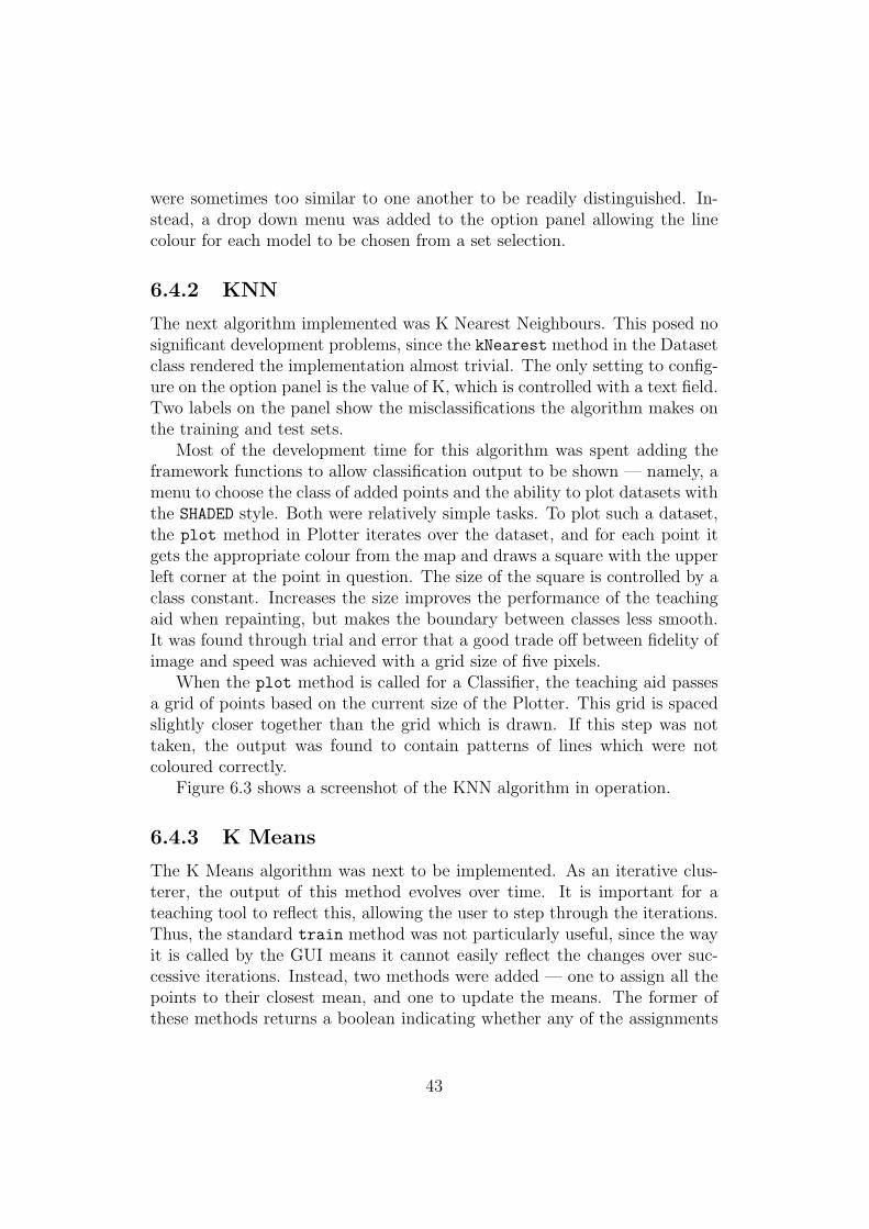
were sometimes too similar to one another to be readily distinguished. In-stead, a drop down menu was added to the option panel allowing the linecolour for each model to be chosen from a set selection.
6.4.2 KNN
The next algorithm implemented was K Nearest Neighbours. This posed nosignificant development problems, since the kNearest method in the Datasetclass rendered the implementation almost trivial. The only setting to config-ure on the option panel is the value of K, which is controlled with a text field.Two labels on the panel show the misclassifications the algorithm makes onthe training and test sets.
Most of the development time for this algorithm was spent adding theframework functions to allow classification output to be shown — namely, amenu to choose the class of added points and the ability to plot datasets withthe SHADED style. Both were relatively simple tasks. To plot such a dataset,the plot method in Plotter iterates over the dataset, and for each point itgets the appropriate colour from the map and draws a square with the upperleft corner at the point in question. The size of the square is controlled by aclass constant. Increases the size improves the performance of the teachingaid when repainting, but makes the boundary between classes less smooth.It was found through trial and error that a good trade off between fidelity ofimage and speed was achieved with a grid size of five pixels.
When the plot method is called for a Classifier, the teaching aid passesa grid of points based on the current size of the Plotter. This grid is spacedslightly closer together than the grid which is drawn. If this step was nottaken, the output was found to contain patterns of lines which were notcoloured correctly.
Figure 6.3 shows a screenshot of the KNN algorithm in operation.
6.4.3 K Means
The K Means algorithm was next to be implemented. As an iterative clus-terer, the output of this method evolves over time. It is important for ateaching tool to reflect this, allowing the user to step through the iterations.Thus, the standard train method was not particularly useful, since the wayit is called by the GUI means it cannot easily reflect the changes over suc-cessive iterations. Instead, two methods were added — one to assign all thepoints to their closest mean, and one to update the means. The former ofthese methods returns a boolean indicating whether any of the assignments
43

Figure 6.3: The KNN algorithm — the output is the shading showing thepoints classified as red, blue or green
changed, which is used to check for convergence of the algorithm. The con-troller class, KMeansPanel, has a ‘Next Iteration’ button that calls each ofthese methods once when it is clicked. After some initial testing, the projectsupervisor suggested the addition of a second button to jump to the solutionat convergence. This allows users to quickly test a given value of K.
The colours for the clusters were initially assigned randomly each timethe algorithm started clustering. This worked reasonably well in some cases,but in others the colours were too similar and it was extremely difficult todistinguish between clusters. As a compromise measure, the first five clusterswere assigned fixed colours so they could always be easily distinguished. Anysubsequent clusters are coloured randomly.
As well as training differently from other algorithms, it was found thatKNN requires a different type of output. The algorithm communicates itsoutput primarily by colouring the training data. The getOutput method re-turns a dataset showing the means. This dataset has the style POINTWISE LARGE,so the means are drawn as circles three times larger than standard points.
44

This enables them to be clearly identified as separate from the data.The semantics of testing are not well defined for clustering in the teaching
aid. No obvious performance measure exists to evaluate on the test set, socurrently nothing is done. This is an area for future improvement to thesoftware.
Figure 6.4 shows the K Means algorithm in operation.
Figure 6.4: The K Means algorithm — the algorithm has found four clustersin the data, with the means represented as large points
6.4.4 SVM
With the three basic types of algorithm represented in the teaching aid, thedevelopment was free to choose any type of algorithm to add. The require-ments gathering exercise suggested that students on the machine learningcourse found SVM to be one of the most conceptually challenging algorithmson the syllabus, so it was a high priority for addition. If a viable quadratic
45

programming solver had been available, it would have been fairly straight-forward to implement an SVM, but without one the proposition was morechallenging. Thankfully, the project supervisor proposed the SMO algorithmas a strong alternative. Implementing this algorithm required a fair amountof work, but still less than an entirely new QP solver.
The full details of the SMO algorithm are beyond the scope of this report,but the basic concept is that pairs of Lagrange multipliers are optimizedanalytically, as opposed to the QP approach which solves numerically for allthe multipliers at once. The SMO approach thus scales much better withthe size of the training data, and in some cases has been shown to be severalorders of magnitude faster than competing algorithms. The modificationproposed by Keerthi et al [15] is what the class SVM actually implements— this improves on several small deficiencies of the SMO technique, furtherincreasing the speed of convergence.
Keerthi et al suggest that the implementation should maintain five sets,I0 to I4, which represent subsets of the αn that meet certain conditions.However, writing the code to add and remove values from these sets seemsoverly complex, particularly given that the conditions for membership ofany the sets amount to two equality tests on primitive types. Thus, theteaching aid implementation replaces these five sets with methods which testa given α to see if it meets the conditions for the corresponding set. Thiswas much simpler than implementing the sets explicitly, and would only besignificantly slower for huge datasets — much larger than the typical setsused in the teaching aid.
SVM was the first kernel algorithm implemented, so a framework forkernel functions was implemented alongside it. This takes the form of aninterface Kernel which specifies a method evaluate. This method takes twopoints x and y and returns the kernel function k(x,y). The teaching aidcurrently specifies three kernels, each represented by a class implementingthe Kernel interface. These are LinearKernel, with
k(x,y) = xTy,
GaussianKernel, with
k(x,y) = exp[−β(x− y)T(x− y)
],
and PolynomialKernel, with
k(x,y) = (1 + xTy)β.
In the Gaussian and polynomial kernels, the additional parameter β is con-trolled by a text field in the option panel.
46
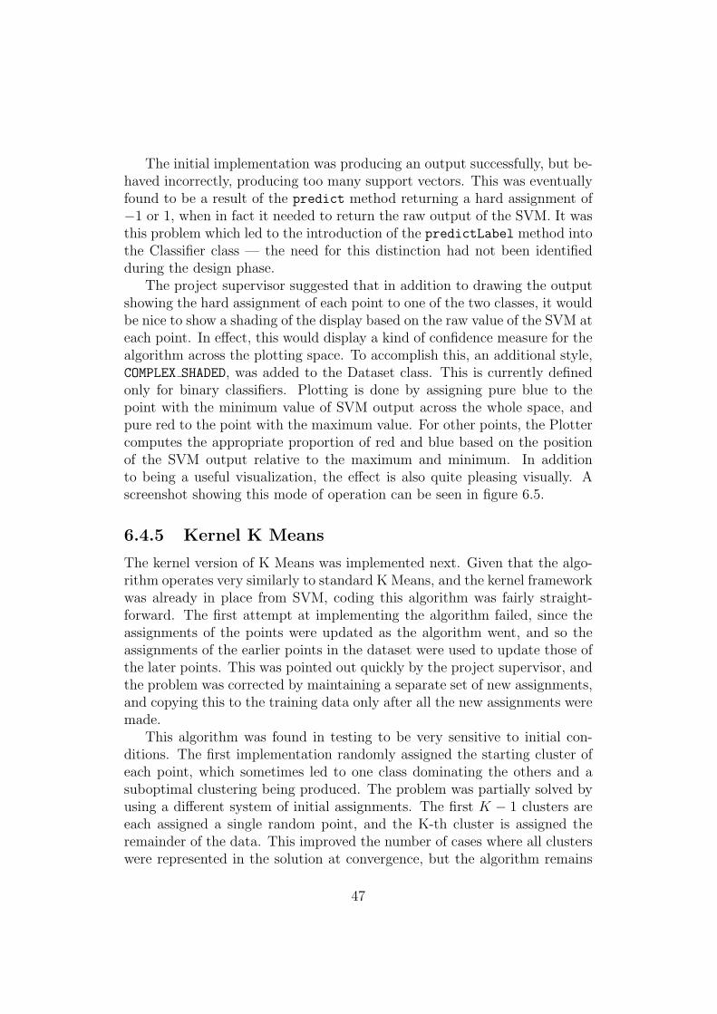
The initial implementation was producing an output successfully, but be-haved incorrectly, producing too many support vectors. This was eventuallyfound to be a result of the predict method returning a hard assignment of−1 or 1, when in fact it needed to return the raw output of the SVM. It wasthis problem which led to the introduction of the predictLabel method intothe Classifier class — the need for this distinction had not been identifiedduring the design phase.
The project supervisor suggested that in addition to drawing the outputshowing the hard assignment of each point to one of the two classes, it wouldbe nice to show a shading of the display based on the raw value of the SVM ateach point. In effect, this would display a kind of confidence measure for thealgorithm across the plotting space. To accomplish this, an additional style,COMPLEX SHADED, was added to the Dataset class. This is currently definedonly for binary classifiers. Plotting is done by assigning pure blue to thepoint with the minimum value of SVM output across the whole space, andpure red to the point with the maximum value. For other points, the Plottercomputes the appropriate proportion of red and blue based on the positionof the SVM output relative to the maximum and minimum. In additionto being a useful visualization, the effect is also quite pleasing visually. Ascreenshot showing this mode of operation can be seen in figure 6.5.
6.4.5 Kernel K Means
The kernel version of K Means was implemented next. Given that the algo-rithm operates very similarly to standard K Means, and the kernel frameworkwas already in place from SVM, coding this algorithm was fairly straight-forward. The first attempt at implementing the algorithm failed, since theassignments of the points were updated as the algorithm went, and so theassignments of the earlier points in the dataset were used to update those ofthe later points. This was pointed out quickly by the project supervisor, andthe problem was corrected by maintaining a separate set of new assignments,and copying this to the training data only after all the new assignments weremade.
This algorithm was found in testing to be very sensitive to initial con-ditions. The first implementation randomly assigned the starting cluster ofeach point, which sometimes led to one class dominating the others and asuboptimal clustering being produced. The problem was partially solved byusing a different system of initial assignments. The first K − 1 clusters areeach assigned a single random point, and the K-th cluster is assigned theremainder of the data. This improved the number of cases where all clusterswere represented in the solution at convergence, but the algorithm remains
47

Figure 6.5: The SVM algorithm — a Gaussian kernel has been used. Rawcolouring mode is shown, and the support vectors are highlighted in white.
sensitive to the random starting positions of the single point clusters. Thisseems to be a deficiency of the algorithm itself, rather than the implementa-tion.
6.4.6 Maximum Likelihood
The final algorithm which was implemented was the maximum likelihoodregression method. This was fairly simple, since much of the code is identicalto that for minimized loss. The optimal parameters are the same, and theoptimal variance is computed in the same way as the average training loss forminimized loss. Thus a lot of the code was reused from the earlier algorithm.However, there were two main differences.
First, the code for adding error bars. For points which errors had beenenabled, the MaxLikelihood version of getOutput sets the size of the error
48

equal to the predictive variance,
vnew = xTnew(cov w)xnew.
Error bars are drawn as vertical bars extending a distance vnew up and downfrom the point, along with two horizontal lines to mark the ends of the errorbar.
Secondly, to compute the likelihood of test sets, it is necessary to eval-uate Gaussians with given means and covariance. To facilitate this, a classGaussian was created that represents a one dimensional Gaussian distribu-tion. The class has methods to set the mean and variance, and to evaluatethe Gaussian for a given x. When computing the likelihood of a Dataset,one of these objects is created for each point, and the values returned bythe evaluate method at each point are multiplier together to produce thelikelihood.
6.5 Sampling Data
Alongside the algorithm implementations, a variety of techniques for generat-ing data were added to the teaching aid. These were added at various pointsduring the development, but the discussion on them is collected here forclarity. For each technique, a class extending the Sampler class was created,specifying an implementation of the nextPoint method.
All of these data generation techniques are controlled via the DataPanelclass. When an option is selected from the drop down menu, the paneldisplays the appropriate configuration options. This is accomplished using aCardLayout, which is similar in function to a tab pane, except that differentviews are selected by a mechanism other than tabs.
6.5.1 Polynomial Sampling
The first data generation technique was sampling from a polynomial. Thisis done by the PolySampler class, and is fairly straightforward. The userspecifies a polynomial order and a value for the noise. The coefficients of apolynomial of the appropriate order are randomly generated. A random xvalue in the range [−10, 10] is chosen, and the value of the polynomial at thatx is computed. The effect of noise is simulated by adding or substracting arandom value, multiplied by the noise value which was previously set. If theresulting t value has |t| > 10, the point is rejected and a new x value is triedto ensure that the sampled data is visible on the plot.
49

The difficulty in implementing this technique arises in scaling the coef-ficients appropriately so that the polynomial which is sampled from is ‘in-teresting.’ In particular, it should have clear turning points in the visibledata range, and should not be too steep. A heuristic that scales the co-efficients so that higher order terms have lower coefficients on average hasbeen implemented, which results in interesting polynomials a fair proportionof the time. There is still room for improvement, however, as some of thepolynomials generated are uninteresting in the plotted space.
Once the desired number of points have been sampled, the coefficientsof the polynomial are randomized again. Previously, a separate button wasincluded to randomize the coefficients, but user feedback suggested that mostusers would only want to sample from a given polynomial once anyway.
6.5.2 Gaussian Sampling
The class GaussianSampler implements sampling from a two dimensionalGaussian distribution. The mean vector and covariance matrix of this Gaus-sian are set by clicking and dragging on the display to draw an ellipse. Forsimplicity, only ellipses with axes orthogonal to the plot’s axes can be drawn.These correspond to Gaussians with diagonal covariance matrices. Once theuser finishes dragging, the mean is set to the center of the ellipse and thediagonal components of the covariance to the sizes of the semimajor andsemiminor axes.
The particular sampling algorithm implemented is taken from [10]. If zis a vector of independent normally distributed values, µ is the mean of theGaussian, and Σ is the covariance, then a vector d which is a sample fromthe Gaussian can be produced by
d = µ + Az.
Here, A is the lower triangular matrix produced by the Cholesky decompo-sition of Σ. Since Java’s Random class provides a method nextGaussian,it is trivial to create z. The Jama matrix library is able to do a Choleskydecomposition, and so this sampling algorithm was easy to implement.
6.5.3 Polygon Sampling
The project supervisor expressed an interest in being able to generate datafrom inside a user specified polygon. It was unclear how feasible this was,but on inspection of Java’s graphics API, the class Polygon was found. Thisrepresents a set of points joined in order to create a polygon. It includes
50

a method to test if a given point is inside the polygon or not, which is thedifficult part of sampling from a polygon. Additionally, the Graphics classhas a method to draw a polygon, so no additional code is needed for that.
The teaching aid implements this function by allowing users to click onthe display to define the vertices of the polygon. When the user clicks thebutton to generate data, the application simply samples random points inthe plotting space, keeping those which fall inside the polygon and rejectingothers, until the requisite number of points is generated. This rejection sam-pling technique is fairly inefficient, but given the speed of modern computers,the process still takes a very short time. This technique is a very powerfulone, allowing data to be produced from very complex shapes with minimaleffort.
One main difficulty arose in implementing polygon data generation. Thiswas related to the fact that the Polygon class only accepts points with integercoordinates. The first implementation simply kept a direct reference to thepolygon, and so when the display was resized, the polygon did not resizewith it. To overcome this problem, the PolygonSampler class was altered toact as a ‘wrapper’ for the Polygon object. A list of points in the data spacewas maintained, and the integer vertices of the polygon were recomputedeach time the Plotter was resized. An unavoidable side effect of this wasthat PolygonSampler had to maintain a reference to the Plotter, so that datacould be transformed back and forward between integer and data coordinates.This introduced an undesirable coupling into the design, but was the onlyapparent way to add the functionality correctly.
6.6 Data storage
The final use cases to be implemented were those concerning the storage ofdata. The ability to save and reload datasets was added, along with theability to export an image of the plot. All of these functions are accessed inthe application through the File menu.
6.6.1 Saving/Loading Data
The ability to save and load data is a useful one. It allows users to keep arecord of interesting datasets they have found, and share them with otherusers if they wish. Datasets are saved to text files using the custom *.dsetextension. A specification of this format is given in appendix D.
Files are loaded and saved by the FileManager class in the io package.This class consists of several static methods — one for writing a dataset
51

to file, one for reading a dataset from file, and one for reading from anInputStream object. The last of these is used to ensure that it is possible toload files located inside a JAR file. The implementation details are relativelyuninteresting — saving involves iterating over the Dataset and writing thedetails of each point to the file, and loading parses the file and extracts therelevant details, creating a Datapoint for each line of the file.
6.6.2 Example Datasets
As well as allowing the user to save and load their own files, this functionalityis used to package a number of interesting datasets directly into the teachingaid. These are accessed through the data generation panel, and include var-ious cases where the algorithms ‘break’. This allows useful examples to be acore part of the application rather than requiring users to obtain the examplefiles themselves. The example datasets are simply .dset files located insidethe JAR files for the program. These are accessed using the FileManagerclass, just as for standard files.
6.6.3 Exporting Images
Finally, a facility for exporting images of the current state of the Plotter wasadded. This was added as a “would like to have” requirement, as it was un-clear how easy or difficult the task would be. Fortunately, it proved very easyas Java as a number of built in features supporting the creation of images.The method is as follows: create an object of the BufferedImage class, getits Graphics object, call Plotter’s paintComponent method on that Graphicsobject. Finally, using the static ImageIO.write method, the BufferedImagecan be written to one of a number of file formats. This process is also carriedout by a static method in the FileManager class. Currently, the teachingaid only supports saving the display in the PNG format. This decision wastaken because PNG is a lossless format, and produces a good representationof the plot. Other formats could easily be added in the future, however.
52

Chapter 7
Testing and Evaluation
An important part of any software development exercise is testing. For thisproject, the testing took two main forms. First, continuous system testingthroughout the development. This was used to ensure that individual codeentities were functioning as intended. Secondly, at the end of the implemen-tation phase a user evaluation took place. The purpose of this was twofold— to assess the performance of the teaching aid against the original require-ments, and to allow a representative sample of end users to try the finalprogram and obtain their feedback. A discussion of both types of testing ispresented below.
7.1 System Testing
One of the main goals of testing is to expose and remove as many defects aspossible from the program. The value of testing is particularly emphasisedin agile software development methods. Since the project was developedusing an agile, incremental model, regular integration and testing was donethroughout the implementation process. After each new piece of functionalitywas written and added to the GUI, it was tested as fully as possible beforemoving on to the next feature.
For the machine learning algorithms, the project proposal called for unittests to be written to check that each algorithm produced the correct out-put. To do this, a test set must be produced and the algorithm’s on the setcomputed externally — either by hand or using another software implemen-tation which is known to be correct. A Java framework, JUnit, exists forwriting unit tests and making assertions about the state of a program aftera specific series of method calls. The initial test plan involved writing a suiteof JUnit tests for each algorithm, and ensuring that it passed all its tests
53

before moving to a new phase of the development.The problem with this is that creating good test sets and evaluating the
output externally to the teaching aid is very time consuming. For regressionmodels, this was manageable. It is reasonably simple to generate data from aknown polynomial, then train a regression algorithm on those data and checkthat the parameters match those of the original polynomial. Indeed, this wasdone for the minimized loss algorithm, and the implementation proved to becorrect.
However, with other algorithms the process of creating validation sets ismuch more difficult. Hand executing an SVM, for example, is a dauntingprospect. Even using a program such as MATLAB to generate the datatakes time, since processing must be done to get the data into a format theteaching aid will recognise. Given more development time, this would bepossible and algorithm correctness could be checked formally, but for thepurposes of the project it was decided unit testing was infeasible.
Instead, system testing took the form of regular user tests by the author.After each change, the program was run and time was spent trying out thenew feature. Additionally, the program was demonstated to the project su-pervisor on a weekly basis, and he also tested it. In this way, the variousconfiguration options for each algorithm were tested using a number of dif-ferent settings. This relied on the expert knowledge of the testers to assesswhether an algorithm was working or not. This is one of the biggest potentialweaknesses of the project as a whole — there is no definitive evidence thatany one implementation is correct. However, given that the algorithms allappear visually to be performing as they should, and respond to parameterchanges in the expected fashion, the risk posed by this less formal testingprocedure appears to have been avoided.
In addition to testing the logic of individual features, testing was carriedout to ensure the program is robust against malformed input — in eachinstance where the user is asked to provide input though a text field, the valuesupplied is checked to ensure that errors are identified and communicated tothe user in a useful fashion. Each text field has been tested with a variety ofinputs, both correct and incorrect, and the program has passed all of thesetests.
The system testing as a whole was successful, in that no major bugs orfaulty logic is exhibited in the final software deliverable. All of the originaluse cases can be performed without incident in the teaching aid, so therequirements are validated.
54

7.2 User Evaluation
The development of the teaching aid concluded with a user evaluation. Theprimary aims of this were:
• To investigate how easily users were able to perform a selection of tasksin the application
• To identify any bugs which had been missed during the implementation
• To gain general feedback about any aspects of the program which weredifficult to understand.
A total of eight users took part in the evaluation. Of these, three were for-mer Machine Learning (M) students, three indicated other previous machinelearning experience, and two had no machine learning experience at all. Thelast group were included in the evaluation to provide an indication of thesystem’s usability from the perspective of a novice. Additionally, having noprior experience of the concepts of the subject, they were able to provide un-biased commentary on the quality of the help files built into the application.
7.2.1 Methodology
The evaluation gathered information in a number of ways, each of which isdiscussed below.
Task List
Participants were first given a document introducing the layout of the teach-ing aid and explaining the basic steps to run an algorithm. With this in-formation, evaluators are then presented with a task list to work through.The tasks include generating data using each of the available methods, andtrying each of the implemented algorithms using a variety of settings. Usersare also asked to read some of the help files, and to use the file handlingcapabilities of the teaching aid to ensure they work.
The tasks on the list are kept fairly general in their wording — this wasto assess how obvious it was to each user which control related to each partof the functionality.
Direct Observation
In conjunction with the task list, the participants were observed as theyused the application and notes were taken on any occasions where they were
55

unsure how to proceed, and on any bugs they encountered. If they wereunsure, participants were encouraged to “think aloud” about the process ofnavigating over the GUI to find the correct option. This provided insightinto a number of usability issues. If they were unable to find the correct wayto proceed, participants were directed to the help files.
Questionnaire
After working through the task list, participants were asked to fill out a shortquestionnaire. The questions were not designed to be analysed in great sta-tistical detail. Rather, their purpose was to gain a sense of the participant’soverall impressions of the teaching aid and to prompt further discussion. Thequestions posed and the responses collected are discussed in the next section.The task and an unfilled questionnaire can be seen in appendix C.
Interview
The evaluation ended with an informal interview. No set questions wereasked. Instead, participants were invited to discuss their questionnaire re-sponses to gain a more detailed understanding of any issues they faced. Fur-ther, during the interviews a number of comments were raised which did notfit into any other part of the evaluation. Brief notes were taken summarisingthe salient points of these interviews.
7.2.2 Results
Questionnaire Responses
The questionnaire contained two Likert style questions, asking evaluatorsto rate the overall design somewhere between excellent and very poor, andto rate the usefulness of the help files between useless and very useful. Allrespondents rated the design either very good or excellent, indicating thatthe majority of tasks were simple and intuitive to perform but that somerequired additional help. The help files were primarily deemed useful, with afew participants opting for very useful. The general consensus is that the helpfiles provide a good accompaniment to the main application. One evaluatorexplicitly noted in the questionnaire that although they did not understandthe mathematical content of the machine learning material, the help filesstill provided them with a better understanding of what the algorithms weredoing.
Another question asked if users were able to complete all tasks on thelist — encouragingly, all evaluators indicated that they were. Additionally,
56

all users who had previous machine learning experience indicated that theythought the application was a good introduction to the basic concepts itcovers. All the MLM students who took part in the evaluation indicatedthat the teaching aid would have been beneficial to them during the course.
However, not all users completed the task list without encountering atleast one unexpected error. A description of some of the issues encounteredfollows.
Bugs
A number of bugs were encountered by the evaluators. These included:
• If a regression model was trained, and the points cleared, it becameimpossible to plot the vertices of a polygon. Erroneous error messageswere displayed after each mouse click.
• When dragging to define a Gaussian, dragging up and to the rightor down and to the left did not work correctly. A straight line wasproduced instead of an ellipse.
• If the radio button for choosing the active dataset is set to ‘Test points’when a new algorithm is set, the setting is not changed back to ‘Trainingpoints’ correctly. This leads to algorithms appearing to break.
• If the user attempts to sample from a polygon without first definingthe shape, the program crashes.
• When changing to a new data generation technique, if there is alreadyan ellipse or polygon drawn on the screen, it does not clear until thedisplay is clicked.
• When adding a new regression model, the new tab is not automaticallyfocused.
• The labels showing the misclassification data for KNN and SVM didnot update from 0/0.
The majority of these bugs were due to small errors in the logic of the pro-gram. These have all been fixed in the delivered version of the teaching aid.The only exception is the last item, regarding the misclassification labels.This error seems to be specific to the machines in the MSc lab where most ofthe evaluations were carried out. It was not possible to reproduce the erroron either of the machines primarily used for development, and the error did
57

not occurs in evaluations conducted in locations other than the lab. The ex-act cause of the problem remains unclear, as insufficient time was availablein the lab to debug the issue.
Comments and Observations
In addition to highlighting defects in the program, the evaluations raised anumber of interesting comments about the design and suggestions for im-provement. These are summarised below.
The single most common design issue raised was that users expectedthe plotted polygon or ellipse to clear after data was generated. The ini-tial design left the objects in place, in case users decided they wanted morepoints from the previous distribution. In practice, none of the evaluatorsused the functionality in this way, and many encountered confusion whenthey attempted to draw a new polygon only to have the existing one ex-tended instead. The feedback with regard to this was so overwhelming thatthe implementation was changed to match the user suggestion. One evalu-ator additionally suggested that on a related point, there was no need forthe polynomial data generator to have a separate button to randomize thecoefficients. Users would only sample from a given polynomial once, so thecoefficients should randomize automatically after generation. This changewas also implemented.
It was suggested that the help files should be rewritten to show a clearerdelineation between the theoretical aspects of an algorithm and the detailsof its implementation in the teaching aid. This is a valid concern. The helpfiles were written in HTML, since Java offers the ability to parse and displayHTML files natively. However, this made it difficult to include mathematicalnotation, since the default implementation is unable to parse MathML. Thus,the files were kept to plain text as far as possible, which led to some intermin-gling of the two details. No changes were made as a result of this comment,but an improvement of the help files would be a useful future extension ofthe project.
On a related note, some users felt that having the help files displayed ina separate window was not optimal, and they would have preferred to havethe help shown in one of the free parts of the layout. This is another possiblecandidate for future work.
A general observation made by a number of evaluators was that the datageneration aspects of the GUI were harder to use than the algorithmic parts.In particular, several were unclear about the exact purpose of the train/testdataset selector, and others did not realise immediately how to change theclass of new points. The common expectation was that all options related
58
to data would be in one panel, and so users were unclear as to the reasonfor the ‘Points’ subpanel. Enough people raised these concerns to warranta possible redesign of the interface in the future, perhaps merging the twosubpanels into one larger structure.
Several users highlighted the known issue that polynomial data are some-times sampled from ‘uninteresting’ functions. This reinforces the need toimprove this feature in the future.
One evaluator expressed an interest in an option to turn off the automaticretraining after new points are added, and instead have retraining done onlywhen the appropriate button is pushed. This is one of the few points raisedby the evaluation that I actively disagree with. One of the primary ideasbehind the teaching aid is that it allows users to explore changes to modelsin real time. If retraining could be turned off, the state of the model wouldbecome out of alignment with what the user might expect given the data.This feature would likely be visually confusing, and this should be avoided.
It was suggested that functionality be added for saving the settings of analgorithm alongside a dataset so that the two could be loaded together asa complete worked example. This is an excellent suggestion, which had notpreviously been considered. There was insufficient time to add such a featurebefore the deadline, but adding this would be an excellent future addition tothe teaching aid.
The final suggestion for improvement that came from the evaluations wasa request for a session history function. This would allow users to move backthrough the history of algorithms and datasets they have used during thecurrent session, in case they wish to recover an interesting case but forgot tosave the data or cannot remember what settings were used for the algorithm.This would take a significant investment of time to implement, but could beuseful.
Not all the comments received were criticisms or suggestions for improve-ment. Encouragingly, a number of users praised the visual design of theteaching aid and expressed a strong belief in its usefulness. In particular,one person commented that the use of shading to show classification outputwas very instructive, and was much clearer than other diagrams they hadseen previously. This is a good indicator that this particular design choicewas the right one.
59

Chapter 8
Conclusion
8.1 Project Status
From the outset, this project had a clear aim: to implement a program toteach basic machine learning concepts. This goal has been achieved. The finalversion of the teaching aid is a robust, well implemented piece of software,and it meets all of its original requirements. User evaluation has indicatedthat the program is simple to use, and has substantial merit as a didactictool.
The project proposal called for a modular, extensible design, which hasbeen achieved through the use of inheritance structures to define the requiredfunctionality for algorithms. The logic of implementing an algorithm is sep-arate from the user interface, which means the GUI can easily be upgradedwithout extensive changes to the domain model. The interface classes ex-hibit a degree of coupling, but this is very hard to avoid in a graphical userinterface. Aside from this, the design makes good use of object orientation todefine focused, cohesive classes which are organized in a clear, logical packagestructure.
While a number of challenges arose during the development, none of theseproved insurmountable, and the final product is free from ‘deep’ errors. Thereis certainly room for the teaching aid to expand and improve in the future,but as it stands the software offers a solid introduction to a variety of machinelearning techniques, and the project can be deemed a success.
8.2 Outstanding Issues
There is one major outstanding issue in the teaching aid as it stands —the look and feel. It was decided that the program would be set to use the
60

system look and feel, which is different across different operating systems,rather than the consistent but unappealing Java look and feel. The evaluationhas highlighted that while the program runs fine on all platforms it has beentested against, there are a number of visual deficiencies on OSX. The Appleimplementation of Java uses larger fonts by default than other platforms, soadditional scroll bars appear in undesirable places and some labels are cutoff because Swing classes do not wrap text automatically. Since a Mac wasnot available for regular testing, it was impossible to identify and correct allof these issues.
To allow for this, two versions of the executable JAR file for the teachingaid have been submitted. One uses the system look and feel, which works fineon Windows and Linux. The other uses the Java look and feel. While thisis not particularly attractive, it at least renders in the same way across allplatforms and allows all the information to be seen. Given more developmenttime and access to a Mac, it would be good to correct these GUI errors.
8.3 Areas for Further Work
There are a number of potential areas for further work on the teaching aid.Some of these have already been discussed, but the suggestions are collectedhere for easy reference.
First, and most obviously, more algorithms could be added. Indeed, one ofthe reasons care was taken to produce a modular design was so that someoneelse could extend the project in the future to increase the range of algorithmsit covers. There are a huge number of available machine learning techniques,many of which can benefit from visualization, so there is no shortage ofpotential work in this area.
As well as new algorithms, the data generation capabilities of the teachingaid could also be extended. While the polygon sampling is very flexible andcan be used to approximate other sampling techniques, there are potentiallyother distributions which could be implemented. Also, there is scope for theimprovement of the polynomial generator. A better method of scaling thecoefficients so that interesting data are produced could be found, for exam-ple. Additionally, it could be possible to add nonlinear terms in additionto the polynomial itself. Since the teaching aid can fit sine curves and ex-ponentials, it seems reasonable that it would also be able to generate dataaccording to such a model. This would require some redesign of the interfacefor polynomial sampling.
The fact that the display is constrained to show a particular interval issomething of a limiting factor. A useful extension would be to implement
61

zooming on the plotting space, so that data can be plotted over a wider rangeof values. It would also allow more of a given regression model to be seen, sothat users can gain an intuition of how the predictive performance extendsoutside the range of the data.
The help subsystem is still fairly basic. The quality of the files couldbe improved by adding a MathML or LATEXparser, to allow easy typesettingof mathematics in the files. Also, a redesign of the interface placing thehelp for an algorithm on screen whenever the algorithm is loaded could beuseful. It is currently slightly unwieldy to switch back and forth between theteaching aid and the help window when additional information is required.Indeed, an overhaul of the interface in general could be beneficial. Thecurrent structure of DataPanel, in particular, caused problems for some usersduring evaluations, so a review of that is in order.
Finally, some evaluators had novel ideas for improving the application inthe future. A history feature, though it would probably take a lot of work,would be an excellent enhancement and offer a lot of useful functionalityfor end users. Similarly, the ability to save algorithm settings together withdatasets and load them as worked examples would be a good improvement.
62

Appendix A
Statement of Requirements
A.1 Functional Requirements
Data generation:
• It must be possible to plot a single data point.
• It must be possible to generate a number of points from a given poly-nomial or distribution.
• It must be possible to remove individual points.
• It must be possible to assign the label on a point, for algorithms whichrequire labels.
• It must be possible to distinguish between training and testing pointswhen plotting.
Algorithms
• It must be possible to select an algorithm to run on the plotted data.
• It must be possible to configure any options for the selected algorithm.
• It must be possible to run an algorithm and plot the resulting model.
• It should be possible to view multiple models over the same data setsimultaneously for regression algorithms.
Cross Validation
• It must be possible to compute the performance of an algorithm usingcross validation over the training set (where appropriate performancemeasures exist).
63

• It could be possible to compare the performance of different modelsusing cross validation.
Data storage
• It should be possible to save the training and test sets so they can berecovered later.
• It would be useful to be able to export an image of the current plot.
A.2 Non-functional Requirements
• The system should be developed in Java.
• The interface should be designed assuming a basic knowledge of ma-chine learning
• The interface should be designed to be intuitive and easily usable.
• Algorithm implementations should be as efficient as possible — no al-gorithm should take longer than a few seconds to train on a set of lessthan 1000 points.
A.3 Use Cases
From the requirements above, a number of candidate use cases were ex-tracted. A diagram showing these is included below.
64

Figure A.1: Use Case Diagram
65

Appendix B
Design Documents
This section contains a package diagram showing the overall structure of theteaching aid, followed by a collection of class diagrams showing the individualcontents of the packages. For clarity, instance variables and methods are notshown on these diagrams. To obtain this information, see the Javadoc onthe accompanying CD.
66

Figure B.1: The overall package structure of the teaching aid
67

Figure B.2: The algorithms package
Figure B.3: The data package
68

Figure B.4: The functions package
69

Figure B.5: The gui package
70

Figure B.6: The help and io packages
71

Appendix C
Evaluation Documents
This appendix contains the documents which were presented to participantsof the user evaluation for the teaching aid. These include a basic informa-tion document detailing the operation of the teaching aid, a task list, and aquestionnaire. The original documents were created using Microsoft Word,but for this document have been rewritten in LATEX.
72

C.1 Basic Information Document
The basic layout of the teaching aid application is shown below, with notesshowing the purpose of each section of the interface.
The basic steps to use the program are as follows:
1. Choose an algorithm in the left hand panel
2. Generate some data — either click on the plot or use the options in thebottom panel
3. Configure the options for your chosen algorithm in the right hand panel,then click ‘Train Model’
4. Individual points can be clicked on to remove them. Add or removepoints to see how the output of an algorithm changes
Use these basic instructions to work through the task list on the followingpages. If you need more information about an algorithm or feature, try thehelp files. These are available through the menu by choosing Help -> ShowHelp.
73

C.2 Task List
Minimized Loss
• Plot some data by clicking on the display
• Choose some terms at the right hand side and train a model
• Run cross validation on your model
Maximum Likelihood
• Choose the maximum likelihood algorithm, then generate some datafrom a polynomial
• Choose some terms and train a model
• Add a second model, and change its line colour
• Click the Partition Data button a few times and observe the effect
KNN
• Generate data from a few Gaussians use several different classes forthe points.
• Train a model with K (Number of neighbours) = 1
• Try changing the value of K to see the effect
SVM
• Use the polygon option to generate some data make sure to add bothred and blue points.
• Train the model using a linear kernel
• Change to Raw colouring mode
• Try adjusting the value of C
• Change to a different kernel
• Change the value of the kernel parameter
• Run cross validation
74

K Means
• Plot some data using any method you want
• Click the Start Clustering / Next Iteration button until the algorithmconverges
• Reset the algorithm, then change the value of K and start again.
Kernel K Means
• Load the Concentric Rings example dataset
• Use a linear kernel to cluster the data note that it fails to capture thestructure
• Use a different kernel to cluster the data change the parameters untilyou are able to capture the structure
Other Features
• If you have not used the help system up to this point, please read a fewof the entries now.
• After training a model, try exporting an image of the plot.
• Try saving and reloading a dataset.
C.3 Questionnaire
1. How clear was the design of the teaching aid?
• Excellent — all tasks were easy and intuitive to perform
• Very good — most tasks were easy, but some required additionalyhelp
• Okay — some tasks were easy, some were difficult
• Poor — many tasks were hard to perform
• Very poor — the application was extremely difficult to use
Specific comments on the design, if any?
2. Were you able to complete all the tasks?
75

• Yes
• No
(a) If no, which tasks were you unable to complete?
3. How useful were the help files?
• Very useful — the help text aided my understanding of one ormore features
• Useful
• Not useful
• Useless — the help text failed to clarify one or more problems
Specific comments on the help files, if any?
4. Did you encounter any unexpected errors while using the program?
• Yes
• No
(a) If yes, please describe these errors.
5. Did you take the Machine Learning (M) course as part of your studies,or did you have experience of machine learning before undertaking thisevaluation?
• Yes — MLM student
• Yes — other previous experience
• No
(a) If yes, do you think the teaching aid offers a useful introductionto the concepts it covers?
• Yes
• No
(b) If you took the course, would the teaching aid have been useful toyou in lectures and lab sessions?
• Yes
• No
6. Suggestions for improvement / Any other comments
76

Appendix D
Dataset file format
Datasets are saved to file with the .dset extension. The file format is plaintext, with a very basic format.The first line of the file contains ‘#Dataset’ and nothing else.The second line of the file contains ‘#size:’ followed by the number of pointsin the dataset.The third line of the file contains ‘#Num classes:’ followed by the numberof distinct labels on the points of the dataset.Each subsequent line of the file represents 1 datapoint. Each line has threedouble values, separated by spaces. In order, these are the x coordinate, they coordinate, and the label of the point.
77

Appendix E
Contents of Accompanying CD
The CD accompanying this dissertation contains a number of folders. Asummary of the contents of these is presented below.
Reports:This folder holds a PDF copy of this dissertation, along with a copy ofthe original project proposal.
Documentation:This folder contains the Javadoc output generated from the teachingaid code.
Source Code:This folder contains the Java source code for the teaching aid applica-tion.
Executables:This folder contains two JAR files. teachingaidfinal.jar is an exe-cutable for the teaching aid, using the system look and feel.teachingaidfinalJ.jar is the same executable, but using the Javalook and feel.
Diagrams:This folder contains full size versions of all the diagrams included inthis report.
78

Bibliography
[1] T. Abeel, Y.V. de Peer and Y. Saeys, Java-ML: A Machine LearningLibrary, Journal of Machine Learning Research, 2009, 10, 931-934
[2] Apache Software Foundation, Apache Commons Math, Available at:http://commons.apache.org/math/
[3] CERN, Colt Project, Available at: http://acs.lbl.gov/~hoschek/
colt/
[4] Chih-Chung Chang and Chih-Jen Lin, LIBSVM : a library for supportvector machines, 2001, Available at: http://www.csie.ntu.edu.tw/
~cjlin/libsvm
[5] Dai Clegg and Richard Barker, Case Method Fast-Track: A RAD Ap-proach, Addision-Wesley, 1994
[6] Jeff De Luca, Feature Driven Development, Available at: http://www.
nebulon.com/fdd/index.html
[7] Donald W. Denbo, Scientific Graphics Toolkit, NOAA/PMEL/EPICGroup, Available at: http://www.epic.noaa.gov/java/sgt/
[8] End of the World Productions, Machine Learning Applets, Available at:www.theparticle.com/applets/ml/index.html
[9] Andreas Geiger, Gaussian Processes for Machine Learning Java Applet,Available at: www.rainsoft.de/projects/gausspro.html
[10] Andrew Gelman, John B. Carlin, Hal S. Stern, and Donald B. Rubin,Bayesian Data Analysis, CRC Press, 2003
[11] Donald Goldfarb and Ashok Udhawdas Idnani, A Numerically StableDual Method for Solving Strictly Convex Quadratic Programs, Mathe-matical Programming, 1983, Vol. 27, pp. 1-33
79

[12] Mark Hall, Eibe Frank, Geoffrey Holmes, Bernhard Pfahringer, PeterReutemann, and Ian H. Witten, The WEKA Data Mining Software:An Update, SIGKDD Explorations, 2009, Volume 11, Issue 1
[13] Kim Hansen, JavaOctave, Available at: http://kenai.com/projects/javaoctave/pages/Home
[14] Hang Tong Lau, A Java Library of Graph Algorithms and Optimization,CRC Press, 2007
[15] S. S. Keerthi, S. K. Shevade, C. Bhattacharyya, and K. R. K. Murthy,Improvements to Platts SMO algorithm for SVM classifier design, Tech-nical Report CD-99-14, National University of Singapore, Available at:http://guppy.mpe.nus.edu.sg/~mpessk
[16] The Mathworks Inc., MATLAB, Natick, Massachusetts, 1984-2010
[17] The Mathworks Inc. and the National Institute of Standards and Tech-nology, JAMA, Available at: http://math.nist.gov/javanumerics/
jama/
[18] Object Refinery Limited, JFreeChart, Available at: http://www.
jfree.org/jfreechart/
[19] Octave Development Community, GNU Octave, Available at: www.
octave.org
[20] John C. Platt, Fast training of support vector machines using sequentialminimal optimization, Advances in Kernel Methods: Support VectorMachines, MIT Press, December 1998
[21] Trygve Reenskaug, Thing-Model-View Editor: An Example From aPlanning System, Xerox PARC Technical Note, May 1979
[22] Simon Rogers and Mark Girolami, A First Course in Machine Learning,CRC Press, 2010
[23] Junjie Sun and Leigh Tesfatsion, QuadProgJ, 2006, Available at: http://econ2.econ.iastate.edu/tesfatsi/DCOPFJHome.htm
80