a low cost localization solution using a kalman filter for data fusion
TRANSCRIPT

A Low Cost Localization Solution Using a KalmanFilter for Data Fusion
Peter Haywood King
Thesis submitted to the faculty of the Virginia Polytechnic Institute and StateUniversity in partial fulfillment of the requirements for the degree of
Master of Sciencein
Mechanical Engineering
Dr. Alfred L. WicksAssociate Professor of Mechanical Engineering
Virginia Tech
Dr. Charles F. ReinholtzAlumni Distinguished Professor, Virginia Tech
Chair, Mechanical Engineering, Embry-Riddle Aeronautical University
Dr. Dennis W. HongAssistant Professor of Mechanical Engineering
Virginia Tech
December 8, 2006Blacksburg, Virginia

A Low Cost Localization Solution Using a Kalman Filter for Data
Fusion
Peter Haywood King
ABSTRACT
Position in the environment is essential in any autonomous system. There are many ways tolocalize and many sensors that provide the data. This paper presents a simple way to systemati-cally integrate sensory data to provide a drivable and accurate position solution. The data fusion ishandled by a Kalman filter tracking five states and an undetermined number of asynchronous mea-surements. This approach takes advantage of the short-term accuracy of odometry measurementsand the long-term fix of a GPS unit. The filter is tested using a suite of inexpensive sensors andthen compared to a differential GPS position. The output of the filter is indeed a drivable solutionthat tracks the reference position remarkably well.

AcknowledgmentsI would like to first thank my parents for their support over the years. The quarter-century of
blind faith has been a gift and is truly appreciated.I would also like to thank my advisors here at Virginia Tech: Dr. Wicks, Dr. Hong, and
especially Dr. Reinholtz. Without the mentorship of these men my academic journey would havebeen unexciting and short-lived.
inally I would like to thank my colleagues here at Virginia Tech past and present for all thefun amidst the toil. I would specifically like to thank Andrew Bacha, Sean Baity, Brett Gombar,and Mike Avitable for their inspiration and advice as I began my work with unmanned systems.Thanks to Jesse Farmer and Jon Weekley who worked along side me, kept me honest, and did notlet me work too hard.
iii

Contents
Chapter 1: Introduction 11.1 Thesis Overview . . . . . . . . . . . . . . . . . . . . . . . . . . . . . . . . . . . 11.2 Motivation . . . . . . . . . . . . . . . . . . . . . . . . . . . . . . . . . . . . . . . 2
Chapter 2: Base Vehicle 42.1 Intelligent Ground Vehicle Competition (IGVC) . . . . . . . . . . . . . . . . . . . 42.2 Virginia Tech Vehicle - Johnny-5 . . . . . . . . . . . . . . . . . . . . . . . . . . . 6
Chapter 3: Background 93.1 Positioning . . . . . . . . . . . . . . . . . . . . . . . . . . . . . . . . . . . . . . 9
3.1.1 Dead Reckoning . . . . . . . . . . . . . . . . . . . . . . . . . . . . . . . 103.1.2 Global Positioning System . . . . . . . . . . . . . . . . . . . . . . . . . . 12
3.2 Kalman Filter . . . . . . . . . . . . . . . . . . . . . . . . . . . . . . . . . . . . . 143.2.1 Background . . . . . . . . . . . . . . . . . . . . . . . . . . . . . . . . . . 143.2.2 Linear Kalman Filter . . . . . . . . . . . . . . . . . . . . . . . . . . . . . 173.2.3 Extended Kalman Filter . . . . . . . . . . . . . . . . . . . . . . . . . . . 183.2.4 Error Modeling . . . . . . . . . . . . . . . . . . . . . . . . . . . . . . . . 193.2.5 Redundant & Asynchronous Inputs . . . . . . . . . . . . . . . . . . . . . 203.2.6 Uses of the Filter . . . . . . . . . . . . . . . . . . . . . . . . . . . . . . . 20
Chapter 4: Filter Design 214.1 Filter Construction . . . . . . . . . . . . . . . . . . . . . . . . . . . . . . . . . . 21
4.1.1 Assumptions & Effects . . . . . . . . . . . . . . . . . . . . . . . . . . . . 224.1.2 State Formulation . . . . . . . . . . . . . . . . . . . . . . . . . . . . . . . 234.1.3 Model - Predict Stage . . . . . . . . . . . . . . . . . . . . . . . . . . . . . 244.1.4 Measurement - Update Stage . . . . . . . . . . . . . . . . . . . . . . . . . 274.1.5 Structure . . . . . . . . . . . . . . . . . . . . . . . . . . . . . . . . . . . 30
4.2 Filter Features . . . . . . . . . . . . . . . . . . . . . . . . . . . . . . . . . . . . . 32
iv

4.2.1 Self-Control . . . . . . . . . . . . . . . . . . . . . . . . . . . . . . . . . 324.2.2 Dynamic Error Adjustment . . . . . . . . . . . . . . . . . . . . . . . . . . 334.2.3 Interface . . . . . . . . . . . . . . . . . . . . . . . . . . . . . . . . . . . 34
Chapter 5: Results 375.1 Straight Line . . . . . . . . . . . . . . . . . . . . . . . . . . . . . . . . . . . . . 385.2 Curve & Return . . . . . . . . . . . . . . . . . . . . . . . . . . . . . . . . . . . . 405.3 Long & Complex . . . . . . . . . . . . . . . . . . . . . . . . . . . . . . . . . . . 425.4 Dynamic Error Adjustment . . . . . . . . . . . . . . . . . . . . . . . . . . . . . . 44
Chapter 6: Conclusion 466.1 Summary of Results . . . . . . . . . . . . . . . . . . . . . . . . . . . . . . . . . . 476.2 Future Work . . . . . . . . . . . . . . . . . . . . . . . . . . . . . . . . . . . . . . 47
6.2.1 Additional Sensors . . . . . . . . . . . . . . . . . . . . . . . . . . . . . . 476.2.2 GPS Bias Correction . . . . . . . . . . . . . . . . . . . . . . . . . . . . . 486.2.3 Zero-Velocity Update . . . . . . . . . . . . . . . . . . . . . . . . . . . . . 486.2.4 Additional Suggestions . . . . . . . . . . . . . . . . . . . . . . . . . . . . 49
References 50
Appendix A: Position-Velocity Example 52A.1 Filter Formulation . . . . . . . . . . . . . . . . . . . . . . . . . . . . . . . . . . . 52A.2 Filter Steps . . . . . . . . . . . . . . . . . . . . . . . . . . . . . . . . . . . . . . 53A.3 Tabulated Position-Velocity Outputs . . . . . . . . . . . . . . . . . . . . . . . . . 61
A.3.1 Q=R, Error = 0 . . . . . . . . . . . . . . . . . . . . . . . . . . . . . . . . 61A.3.2 Q>R, Error = 0 . . . . . . . . . . . . . . . . . . . . . . . . . . . . . . . . 63A.3.3 Q<R, Error = 0 . . . . . . . . . . . . . . . . . . . . . . . . . . . . . . . . 65A.3.4 Q=R, Error = 0.1 . . . . . . . . . . . . . . . . . . . . . . . . . . . . . . . 67A.3.5 Q>R, Error = 0.1 . . . . . . . . . . . . . . . . . . . . . . . . . . . . . . . 69A.3.6 Q<R, Error = 0.1 . . . . . . . . . . . . . . . . . . . . . . . . . . . . . . . 71A.3.7 Modeled Q, Modeled R, Error = 0.5 . . . . . . . . . . . . . . . . . . . . . 73
v

List of Figures
2.1 IGVC Logo. . . . . . . . . . . . . . . . . . . . . . . . . . . . . . . . . . . . . . . 52.2 Johnny-5 on the hillside. . . . . . . . . . . . . . . . . . . . . . . . . . . . . . . . 6
3.1 Differentially driven kinematics . . . . . . . . . . . . . . . . . . . . . . . . . . . 113.2 Ackerman Steered kinematics . . . . . . . . . . . . . . . . . . . . . . . . . . . . 123.3 Kalman Filter process flow . . . . . . . . . . . . . . . . . . . . . . . . . . . . . . 16
4.1 Filter output . . . . . . . . . . . . . . . . . . . . . . . . . . . . . . . . . . . . . . 344.2 Input to filter . . . . . . . . . . . . . . . . . . . . . . . . . . . . . . . . . . . . . 354.3 Error modification . . . . . . . . . . . . . . . . . . . . . . . . . . . . . . . . . . . 35
5.1 Straight line data with no starting point . . . . . . . . . . . . . . . . . . . . . . . . 385.2 Straight line data with starting point . . . . . . . . . . . . . . . . . . . . . . . . . 395.3 Straight line errors . . . . . . . . . . . . . . . . . . . . . . . . . . . . . . . . . . 405.4 Curve & return . . . . . . . . . . . . . . . . . . . . . . . . . . . . . . . . . . . . 415.5 Curve & return error . . . . . . . . . . . . . . . . . . . . . . . . . . . . . . . . . 415.6 Complex path . . . . . . . . . . . . . . . . . . . . . . . . . . . . . . . . . . . . . 425.7 Complex path error . . . . . . . . . . . . . . . . . . . . . . . . . . . . . . . . . . 435.8 Path with no pop protection . . . . . . . . . . . . . . . . . . . . . . . . . . . . . . 445.9 Path with pop protection . . . . . . . . . . . . . . . . . . . . . . . . . . . . . . . 45
A.1 P-V Example: Step 0 . . . . . . . . . . . . . . . . . . . . . . . . . . . . . . . . . 54A.2 P-V Example: Step 1 . . . . . . . . . . . . . . . . . . . . . . . . . . . . . . . . . 57A.3 P-V Example: Step 2 . . . . . . . . . . . . . . . . . . . . . . . . . . . . . . . . . 59A.4 P-V Example: Step 3 . . . . . . . . . . . . . . . . . . . . . . . . . . . . . . . . . 59A.5 P-V Example: Step 4 . . . . . . . . . . . . . . . . . . . . . . . . . . . . . . . . . 60A.6 P-V Example: Step 5 . . . . . . . . . . . . . . . . . . . . . . . . . . . . . . . . . 60A.7 Error: Inputs perfectly known, Q=R . . . . . . . . . . . . . . . . . . . . . . . . . 61A.8 Error: Inputs perfectly known, Q>R . . . . . . . . . . . . . . . . . . . . . . . . . 63A.9 Error: Inputs perfectly known, Q<R . . . . . . . . . . . . . . . . . . . . . . . . . 65
vi

A.10 Error: Inputs ± 10%, Q=R . . . . . . . . . . . . . . . . . . . . . . . . . . . . . . 67A.11 Error: Inputs ± 10%, Q>R . . . . . . . . . . . . . . . . . . . . . . . . . . . . . . 69A.12 Error: Inputs ± 10%, Q<R . . . . . . . . . . . . . . . . . . . . . . . . . . . . . . 71A.13 Error: Inputs ± 50%, Q,R Modeled . . . . . . . . . . . . . . . . . . . . . . . . . 73
vii

List of Tables
2.1 Sensor suite on Johnny-5 . . . . . . . . . . . . . . . . . . . . . . . . . . . . . . . 8
3.1 GPS Solution Comparison . . . . . . . . . . . . . . . . . . . . . . . . . . . . . . 14
A.1 Filter Summary - Inputs perfectly known, Q=R . . . . . . . . . . . . . . . . . . . 62A.2 Filter Summary - Inputs perfectly known, Q>R . . . . . . . . . . . . . . . . . . . 64A.3 Filter Summary - Inputs perfectly known, Q<R . . . . . . . . . . . . . . . . . . . 66A.4 Filter Summary - Inputs ± 10%, Q=R . . . . . . . . . . . . . . . . . . . . . . . . 68A.5 Filter Summary - Inputs ± 10%, Q>R . . . . . . . . . . . . . . . . . . . . . . . . 70A.6 Filter Summary - Inputs ± 10%, Q<R . . . . . . . . . . . . . . . . . . . . . . . . 72A.7 Filter Summary - Inputs ± 50%, Q,R Modeled . . . . . . . . . . . . . . . . . . . . 74
viii

Chapter 1
Introduction
In any unmanned system application, localization is paramount. In any engineering application,
cost is a factor. The balance of these two statements is not trivial. This thesis presents a simple
implementation of a Kalman filter to provide a drivable localization signal at a low cost. Originally
intended for a small autonomous vehicle, the approach was designed to be easily ported to other
platforms.
1.1 Thesis Overview
This thesis presents a way to provide a drivable and accurate position solution using inexpensive
sensors. A Kalman filter is used to fuse that data from these sensors to produce an output that is
better than that of any single sensor. The goal is to provide a cost-effective solution accurate enough
to replace a system that is twenty times the cost. This is another feat for value engineering where
smart software design can replace expensive hardware with little degradation in performance.
This thesis will cover the basics of the Kalman filter along with positioning solutions, present
1

the test platform, describe the formulation of the filter presented, and discuss the results. The
remainder of this chapter will set up the problem and outline the solution. Chapter 2 will then
discuss the specific application of this technology as well as describe the test platform.
Chapter 3 will cover the existing solutions. This includes the relative positioning provided
by the system of Dead Reckoning. The chapter will also present the basics of GPS and some of
the commercially available systems. Finally it will present the Kalman filter, a way to combine
multiple sources of data in an optimal way.
Chapter 4 will cover the topic of the actual design of the filter. The structure, system model,
and measurement scheme will be first. This filter was designed to be robust and for ease of use, so
the interface and additional features will be presented in this section, as well. The resulting output
will be discussed in Chapter 5. The output will be compared to a top-of-the-line system to give
perspective to the overall performance.
1.2 Motivation
The first step in achieving any goal is to assess the current position. While this adage has a broad
reach, it is also applicable to the unmanned arena. When trying to navigate through the world, a
frame of reference must be established. When the frame is outside of the vehicle, there must be a
way of locating that vehicle in this frame. There are many different ways to perceive position and
many ways to measure displacement; the trouble lies in deciphering the massive amounts of data.
To use all of the information properly, there needs to be a way to combine the perceived states
into a single best estimate. Fortunately, the Kalman filter has been around for half a century and is
still one of the best ways to incorporate several inputs regarding a system. This should provide an
excellent shell for a localization solution for an autonomous system.
Many unmanned systems are small and operate in environments that can fall into a simple
model. One such application is in the Intelligent Ground Vehicle Competition (IGVC). In this
competition, mobile robots are asked to perform tasks autonomously and the entries are judged
2

on performance as well as design. Recent advances in robotics have brought control schemes to
the forefront of investigation. In this aspect of the competition, Virginia Tech has excelled, but
engineering is based on many design parameters, not only performance. There is still the problem
of describing the world and making use of the information optimally. This information can come
from many sources and encompass many descriptions. The data can have varying degrees of
accuracy and wide range of cost associated with it.
The filter presented in this work is a method of combining data from several sources to produce
a single estimate of position. To fuse the data, this scheme will use a Kalman filter and exploit the
inherent advantages. The final filter will use the asynchronous input and the optimal estimation
provided by Kalman’s approach to produce a drivable position solution. This is all in the attempt
to use software to eliminate expensive hardware, making an autonomous vehicle even more of an
astonishing feat of engineering.
3

Chapter 2
Base Vehicle
Virginia Tech’s success at the Intelligent Ground Vehicle Competition has put the university in the
fortunate position of pursuing research to achieve the same standard of performance by alternative
means. The effort described here is to replace the expensive GPS unit with a lower cost unit and
resolve the loss of accuracy through the use of data fusion.
The test platform is Johnny-5, an autonomous ground vehicle developed previously by Vir-
ginia Tech for the Intelligent Ground Vehicle Competition (IGVC). Johnny-5 is a three-wheeled,
differentially driven robot with a full compliment of sensors to perform in the IGVC. The rugged
construction, simple dynamics, and integrated sensor suite make it a perfect vehicle for research.
2.1 Intelligent Ground Vehicle Competition (IGVC)
The IGVC is an annual competition for students at the university level. To compete, teams must
design, build, and program an autonomous vehicle to compete in three events: The Autonomous
Challenge, the Navigation Challenge, and the Design Competition[8]. These events are staffed by
4

the sponsoring companies and programs, and judged by professionals from industry. Here the need
for an accurate but inexpensive position solution is brought by the competition parameters and by
the judges’ drive for engineering application.
Figure 2.1: IGVC Logo.
Autonomous Challenge
The Autonomous Challenge is an outdoor obstacle course. Vehicles must stay between lines that
are painted on grass. These lines can colored white or yellow and may be solid, dashed, or missing
altogether. Inside the lines there are obstacles to avoid. These obstacles take the form of traffic
barrels and cones, construction sawhorses, colored garbage bins, ramps, potholes, sand pits, and
trees. Obstacles may be moved between runs and the direction of travel around the course may also
be changed. The event is judged on adjusted time to complete the course. If no one has completed
the course, the furthest adjusted distance traveled wins. The times and distances are adjusted for
traffic violations such as leaving the course, grazing obstacles, etc.
Navigation Challenge
The Navigation Challenge requires the vehicle to visit GPS waypoints. The only information
given is the coordinates of the waypoints. There are many different obstacles that are in the way
including barrels, barriers, fences to name a few. Vehicles must autonomously make it through the
5

field, getting within 1 or 2 meters (depending on the difficulty) of the waypoint. Judging of the
competition is based on the number of waypoints hit and the time it took to reach them.
Design Competition
The Design Competition is the judging of the design process and innovations brought to competi-
tion. The three parts of this competition are an oral presentation, a written report, and an inspection
of the vehicle. The Judges come from various industries and are concerned with the product pro-
duced regardless of dynamic results.
2.2 Virginia Tech Vehicle - Johnny-5
Johnny-5 is an autonomous vehicle created to compete in the Intelligent Ground Vehicle Competi-
tion. In fact, Johnny-5 (shown in figure 2.2) has had a long line of successes at the IGVC. The first
year it was entered (2004), it received the first place overall. In subsequent years it received third
(2005), second (2006), and finally first again in 2007.
Figure 2.2: Johnny-5 on the hillside.
6

Mechanical System
Johnny-5 (J5) is a differentially steered, three wheeled vehicle [7]. The rugged frame is crafted
of aluminum and is a single body housing the electrical, computing and sensing components. The
two drive wheels are independently driven by two brushless DC motors produced by Quicksilver
Control. The output of the motor is reduced by a 10:1 gear head to spin the 15” composite wheels.
Electrical/Computing System
Johnny-5 has a hybrid power system connected in series. A 1000 Watt portable generator powers
the battery charger which, charges the batteries that run the vehicle. All of the sensors and com-
ponents run off either 12 or 24 volts. The compass, Novatel GPS, and the camera all run on the
regulated 12v line, while the SICK Laser Range Finder (LRF) runs on a regulated 24v. The motors
run on an unregulated 24v power line. The computer can also be plugged into the generator to use
the standard AC power supply that comes with the laptop.
The computing on the vehicle is done by a Sager NP8890 laptop. While currently slightly
antiquated, it has proved to be more than adequate to control the vehicle. The laptop processes
all of the data coming in from the sensors by way of serial RS-232 connections. The interface
and navigation is all programmed in LabVIEW by National Instruments. This is a programming
language that is a graphical interface that is instrumental in rapid development of sensors and
control. The data can be ordered graphically and structured in a way that is user friendly. This will
also be the native language for the filter presented later.
Sensor Suite
Onboard, J5 has the necessary components to compete in the IGVC. For line detection as well as
obstacle avoidance, there is a Unibrain R©Fire-i camera mounted on the mast. The primary obstacle
avoidance is the LRF on the front. There is also a Novatel Propak LB that receives Onmistar
HP corrections to determine the position and a PNI 3-axis compass to determine orientation. In
7

addition, the Quicksilver motors are equipped with a relative quadrature encoder. The sensors are
summarized in table 2.1. For this work, Johnny-5 will also be equipped with a Ublox Antaris 4
GPS evaluation unit. This will be used as the position input to the developed filter.
Table 2.1: Sensor suite on Johnny-5
Sensor Measurement ResolutionUnibrain Fire-i camera Vision 640 x 480 pixelsSICK LMS 291 Range 180 degrees, cm accuracyQuicksilver Motor Encoders Motor Rotation 16000 ticks/revPNI Compass Orientation 0.8 degrees accuracyNovatel Propak + OmniStar Position CEP of 10 cmUBlox Antaris 4 Position CEP of 5 m
8

Chapter 3
Background
When designing a position solution, an understanding of the dominant techniques of positioning
and their inherent errors is required. This chapter will discuss positioning and also give some
background into the Kalman filter. This foundation is what will drive the fusion of data into a
position solution that is more accurate and more drivable than any of the inputs by itself.
3.1 Positioning
The question ”Where am I?” has several answers. Likewise with autonomous systems, there are
many ways of positioning a vehicle within an environment. An increasingly common solution is
the Global Positioning System (GPS). This solution will give an absolute position measurement in
reference to the earth. There are also ways of finding a relative position by using Dead Reckoning
(DR). Both techniques have advantages and disadvantages, the goal is to combine them in an
intelligent way to utilize their advantages. This section will cover the basics of positioning as they
are generally applied to autonomous systems.
9

3.1.1 Dead Reckoning
Dead Reckoning is the estimation of the current position based on a previous position, rate of
travel, direction, and time. The model of the motion comes down to the vehicle kinematics. The
method of advancement is the integration over time, thus errors tend to accumulate in the position
solution [3]. This means that the solution is good in the short term, but estimations will probably
diverge over time. This error can come from a number of sources. The vehicle parameters can
be inaccurate (wheel base, wheel diameter, etc.), the measuring technique could be measuring the
wrong thing (wheel slip), or the environment may not be conducive to simplified models (uneven
terrain).
Measurement usually uses some form of odometry. Generally wheel encoders are used, but
there are other methods as well including vision [1]. Wheel encoders are excellent choices for
DR because they are inexpensive and offer high sampling rates. This is desirable because if the
information is going to be combined with other measurements, DR would provide the short-term
accuracy component. The faster the samples, the less room for error.
The velocities can be broken up into two components, forward and rotational. Finding these
components of the velocities is a matter of modelling the motion with respect to the known com-
ponents. For wheel encoders, the wheel speeds are known but the vehicle velocity components are
desired. With different vehicles the way to arrive at these values differ, but there are a few useful
models to understand.
Differential Drive
In a differentially driven vehicle the velocity is rather simple to derive from the wheel speeds using
the instant centers. The concept of an instant center is that at any moment in time, there is a point
around which a rigid body appears to be rotating. The entire system is attached to the rigid body.
Since angular velocity must be conserved, the distance to the instant center from the wheels is used
to determine the angular rate of the rigid body, and then projected to the vehicle’s center of mass.
10

This can be simplified to the equation presented in figure 3.1.
Figure 3.1: Kinematics of a differentially driven vehicle.
The remaining component of wheel velocities is the rotational component. The difference of
the wheel velocities with respect to the average velocity will be the rotating component, but to get
it into the angular rate of the vehicle, divide by half of the track width. This can be simplified into
the form showed in figure 3.1. These are the equations for the velocities of a differentially steered
vehicle given the wheel velocities and the track width of the vehicle.
Bicycle Model
In vehicles that have three driven wheels, or an Ackerman steered vehicle, the model of choice is
the bicycle model. In Ackerman steered vehicles, it is assumed that the front wheels are turned
slightly differently so that the instant centers of each wheel coincide. From this instant center,
an equivalent kinematic model can be produced with one wheel in front and one wheel in back,
mimicking a bicycle. From here, the forward velocity is determined the same as the differential
case. The angular velocity is still a function of the curvature being driven, but it is derived a little
differently [11]. Figure 3.2 shows the formulation of this model.
11

Figure 3.2: Kinematics of an Ackerman steered vehicle.
3.1.2 Global Positioning System
The Global Positioning System (GPS) is a system of 24 satellites orbiting earth in six orbital planes
[9]. This has become the most popular way of positioning with respect to the Earth because of its
ease of use, inexpensive implementation, and wide range of availability. Each satellite broadcasts s
signal from its known position in the sky. The GPS receiver needs four of these signals to be able to
discern the location through time-of-flight calculations. Four signals are needed because accurate,
synchronized clocks are prohibitively expensive so the time is solved for as a fourth variable along
with the three-dimensional position.
The output from a GPS receiver is the solution to the pseudorange equations (from the four
satellites) translated into the output the user can utilize, generally latitude and longitude measure-
ments. Another useful positioning scheme is the Universal Transverse Mercator (UTM) coordinate
system. In this system, the globe is broken up into small zones that are then represented as an x−y
plane, measured in meters. The output of the GPS receiver is prone to errors, but the majority of
these errors are transient effects of the atmosphere. For this reason, GPS is more accurate when
averaged over longer periods of time.
12

Corrections
GPS measurements are subject to a number of sources of error. Disturbances in the atmosphere,
internal clock error, and ephemeris error are all part of the system. There are errors on the user
end as well. Multipath effects and RF interference can also cause distortion or loss of the signal.
Anything that effects the direct line of sight with the satellite will cause position error.
Use of differential corrections can reduce many of the system-level errors. These corrections
are measured by base stations around the world and transmitted back over satellites to be used by
enabled receivers. In the western hemisphere, the Wide Area Augmentation System (WAAS) is
used in this capacity. Designed for aircraft landing at airports, the system’s accuracy is not meant
to be a global solution. OmniStar is another correction signal that is available by subscription. This
is a worldwide correction that offers highly accurate returns.
Products
There are a number of commercially available GPS solutions on the market today. These all range
in price and accuracy as well as the intended application. Handheld receivers can cost anywhere
from $100 up to $600 and can include mapping functions as well as location information. The
error reported by these products is the Circular Error Probable (CEP). This is the radius of the
circle (based at the true value) that contains the measurement 50% of the time.
The Novatel Propak is a commercially available unit intended for high accuracy and built in
communication with an Inertial Measurement Unit (IMU). These features come with a hefty price
tag but, when coupled with the OmniStar correction, render a solution that is accurate with a CEP
of 10 centimeters. Another commercially available unit is the U-Blox receiver. It is an integrated
microchip receiver designed to be integrated into systems, but can be purchased with supporting
circuitry or as complete unit ready for testing. Table 3.1 below lists some products available with
the associated cost and error. The accuracy increases with the price, as would be expected.
13
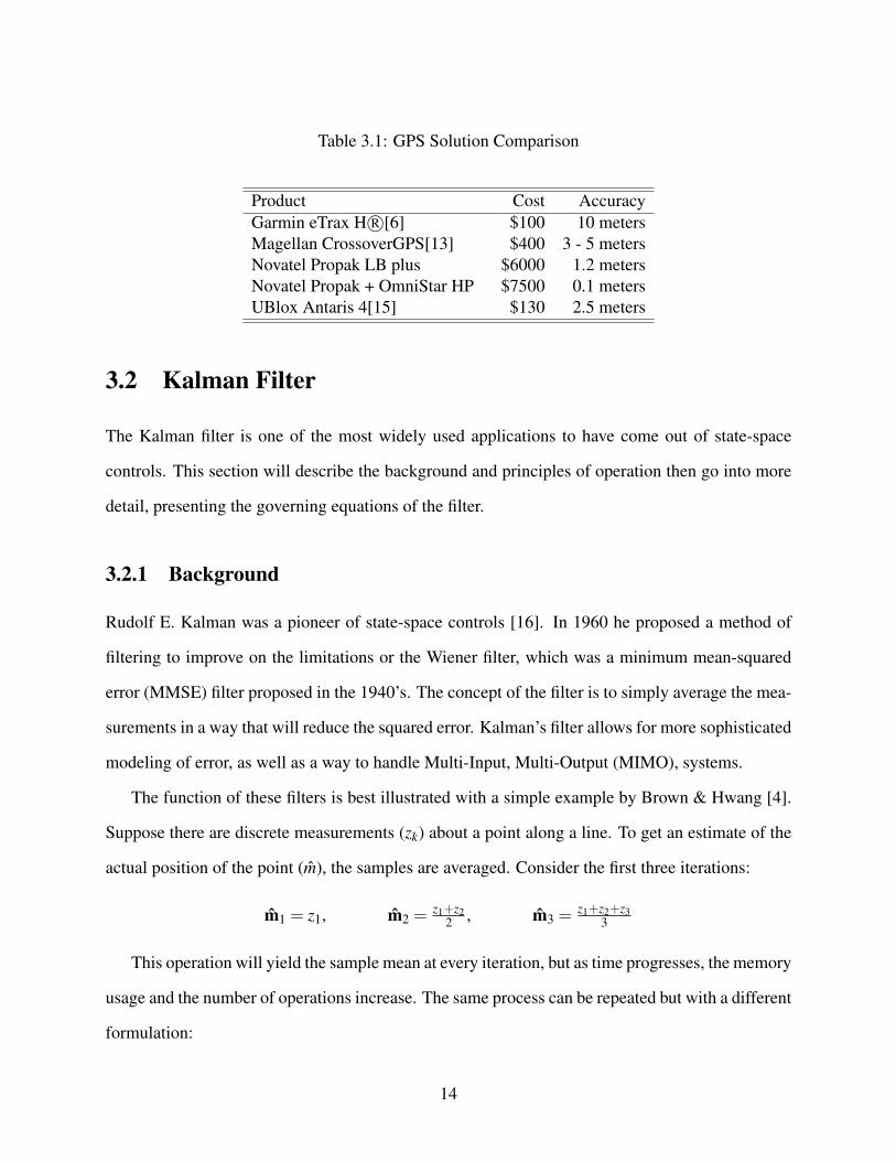
Table 3.1: GPS Solution Comparison
Product Cost AccuracyGarmin eTrax H R©[6] $100 10 metersMagellan CrossoverGPS[13] $400 3 - 5 metersNovatel Propak LB plus $6000 1.2 metersNovatel Propak + OmniStar HP $7500 0.1 metersUBlox Antaris 4[15] $130 2.5 meters
3.2 Kalman Filter
The Kalman filter is one of the most widely used applications to have come out of state-space
controls. This section will describe the background and principles of operation then go into more
detail, presenting the governing equations of the filter.
3.2.1 Background
Rudolf E. Kalman was a pioneer of state-space controls [16]. In 1960 he proposed a method of
filtering to improve on the limitations or the Wiener filter, which was a minimum mean-squared
error (MMSE) filter proposed in the 1940’s. The concept of the filter is to simply average the mea-
surements in a way that will reduce the squared error. Kalman’s filter allows for more sophisticated
modeling of error, as well as a way to handle Multi-Input, Multi-Output (MIMO), systems.
The function of these filters is best illustrated with a simple example by Brown & Hwang [4].
Suppose there are discrete measurements (zk) about a point along a line. To get an estimate of the
actual position of the point (m), the samples are averaged. Consider the first three iterations:
m1 = z1, m2 = z1+z22 , m3 = z1+z2+z3
3
This operation will yield the sample mean at every iteration, but as time progresses, the memory
usage and the number of operations increase. The same process can be repeated but with a different
formulation:
14

m1 = z1, m2 = 12m1 + 1
2z2, m3 = 23m2 + 1
3z3
Here, each iteration is treated as a weighted sum. The estimate is weighted such that the output
is mathematically identical to the arithmetic mean; but between the iterations, the individual mea-
surements are discarded and only the previous estimates are saved for use in future iterations. The
end result is that the current estimate is based on the current measurement and the prior estimate.
To produce an optimal estimate instead of the average, the weighting based off of the iterations
could be replaced with weights assigned by relative uncertainty. In fact, this is what the Kalman
filter does.
The Kalman filter carries the estimate and the weighting to be assigned to the estimate in ma-
trices called the State Matrix and the Covariance Matrix, respectively. The State Matrix contains
the states, or pertinent descriptions of the system. This would be the estimate of position in the
averaging example, but it can also contain information on velocity, heading, anything that is being
monitored, or anything that may be related to what is being monitored. The Covariance Matrix
contains information about how the states vary with respect to each other. The diagonal of the co-
variance matrix is the variance for each state, which is a statistical indicator of the error associated
with that state.
The information follows the flow depicted in figure 3.3. There are two major stages in the
Kalman filter: the update stage and the prediction stage. The output of the filter will be the optimal
combination of the current measurements and the system model based on the prior estimate. This
optimal estimate should not be confused with a more accurate estimate. The filter only has the
information of the system model and the sensory input; garbage in will still be garbage out.
Prediction Stage
In the prediction stage, the states are advanced through time according to a system model. This
model may contain any equation to describe the states. This model is put into its state space
formulation in order to be incorporated into the Kalman filter via the Transition Matrix.
15

Figure 3.3: Data flow of the Kalman filter.
The error produced by the model advancing the states is added to the covariance. This means
that the cost of prediction is more error in the estimate of the state. If there were to be no correction
provided to the model, the error would simply grow. This is the same sort of expectation when a
control system is run open-loop. With no feedback, the states are not perfectly known and the error
continues to accrue until the output is unusable.
Update Stage
The update stage, also called the correction stage, is responsible for updating the predictions with
the measurements that have been acquired. This is the process that will rein in the error and correct
the output states. This correction will be weighted as discussed in the averaging example. This
weight, called the Kalman gain, is based on the uncertainties of the prediction (model-based state)
and the measurements available.
The covariance is then reduced according to the how much the prediction had to be corrected.
As the filter progresses, the measurement and the prediction should reach a point where the reduc-
tion in the covariance in the update step matches the error added by the prediction. At this point
16

the filter is considered converged.
Often times, an example helps understand how the filter operates. Appendix A examines a
simple case of a point along a line.
3.2.2 Linear Kalman Filter
The simplest implementation of Kalman’s work is in the Linear Kalman Filter. This model makes
the assumption that the governing equations are functions of the tracked states. These functions
may be time varying, but the transition matrix, the error model, and the measurement matrix are
all linear functions of the states. This approach can be applied to nonlinear systems, but the mea-
surement matrix and the error propagation will be less accurate.
The prediction stage for the linear phase is a simple matter of stepping the states forward
through time using the Transition Matrix, Φk. This matrix has the equations that make up the
linear model. The covariance is then projected forward by adding the system covariance, Qk,
transformed by the Gamma Matrix, Γ.
X−k = ΦkXk−1 (3.1)
P−k = ΦkPk−1ΦTk +ΓkQkΓ
Tk (3.2)
The update stage is accomplished by Computing the Kalman Gain, correcting the state es-
timate, and then updating the covariance. The Kalman gain (equation 3.3 is a function of the
estimated errors, P−k , the Measurement Matrix, Hk, and the Measurement Uncertainty, Rk. This
forms the ratio of how certain the measurement is in comparison to the prediction. The Kalman
17

gain is then used to correct the state estimate and reduce the state covariance.
Kk = P−k HTk[HkP−k HT
k +Rk]−1
(3.3)
Xk = X−k +Kk[Zk−HkX−k
](3.4)
Pk = [I−KkHk]P−k (3.5)
3.2.3 Extended Kalman Filter
To handle a nonlinear plant, the Extended Kalman Filter (EKF) is used. In reality, it is an extension
of the linear form of the filter. The equations are similar to the Linear Kalman Filter, but in order
to account for the nonlinearities, the Transition Matrix and the Measurement Matrix are linearized
by using the Jacobian of the time derivative. The structure of the filter is going to be comparable to
the Linear Filter, but this linearization allows for nonlinear effects to be properly carried through
the propagation of the filter.
Hk =∂h∂x
(x−k ) (3.6)
Fk =∂ f∂x
(x−k ) (3.7)
where h is now the Measurement Matrix and f is the time derivative of the system model. In the
extended scheme, the covariance will now be modified by this linearized form of the model and
measurement transformations.
In the prediction stage, the state is advanced in the same fashion. The Transition Matrix is
now a nonlinear expression of the model. This is usually written by inspection. The covariance is
projected forward similarly as well, keeping in mind that the transformation has been linearized.
X−k = ΦkXk−1 (3.8)
P−k = FkPk−1KTk +ΓkQkΓ
Tk (3.9)
18

Likewise, the update stage is similar, differing from the linear case by use of the linearization.
Kk = P−k HTk[HkP−k HT
k +Rk]−1
(3.10)
Xk = X−k +Kk[Zk−hX−k
](3.11)
Pk = [I−KkHk]P−k (3.12)
3.2.4 Error Modeling
In both formulations of the filter the error matrices Qk and Rk are functions of the uncertainty. As
the names imply, the state uncertainty matrix, Qk, is a measure of the error in the model and the
measurement uncertainty matrix, Rk, is the uncertainty associated with the measurements. The
uncertainty is described as the expected value of the correlation of the error in the model or the
measurements. In order for the filter to remain consistent, the expected values of the correlation
must be the covariance of the errors. This implies that the errors need to have a normal distribution.
This is the mode of error that will maintain the relationship
E(εi · εT
j)
= σi ∗σ j (3.13)
where i and j represent the indices of the measurement state or system state depending on which
matrix is being formulated. Taking this across the state space forms the covariance. A general
assumption is that the uncertainty across states is uncorrelated, driving the off-diagonal terms of
the covariance matrix to zero. What is left is a matrix where the diagonal elements are the variance
of the state.
The uncertainty matrices are essentially the weights that are applied to the filter that determines
the behavior[10]. The Qk matrix is a description of the error if the system prediction is run open-
loop. As time moves forward, small errors in the model will propagate and increase unbounded.
The Rk matrix is associated with the error in the measurements and is used as in the gain of the
19

corrections.
3.2.5 Redundant & Asynchronous Inputs
Because the Kalman filter is set up as a state space representation, the individual states are kept
separate despite having an effect on one another. This affects the update stage in that the states
that have measurements can be singled out and updated. There is also the benefit of updating a
single state with multiple measurements. The gain function will assign appropriate weights to the
corrections and the filter will automatically select the minimum error between the measurements
and the predicted state.
The problem of asynchrony and redundancy open the problem of data timing. There is latency
from the sensor to the filter. There is latency from the prediction to the update stage. The update
may not happen fast enough. These all effect when data is assumed to be valid. Careful thought
should be applied to the data structure of the platform if data is to be fused together.
3.2.6 Uses of the Filter
The Kalman filter has been in wide use for half of a century. Agrawal and Konolige [1] present
the Kalman filter as a way to fuse visual odometry and an inexpensive GPS in order to provide a
position. Their work seemed like more of a way to validate visual odometry than provide a position
solution, but it is an excellent application of the Kalman filter. Aufrere, et al. [5] effectively used
the Kalman filter in order to localize within a road. The prediction was traveling down the road
and this was updated with measurements of the extent of the road.
The Kalman filter can also be used to provide localization in other schemes as well. By clever
use of the Measurement Matrix, Leaonard and Durrant-Whyte [12] were able to use geometric
beacons and an a priori map to position a mobile robot within a room. The IGVC team from
Bluefield State College used a Kalman filter to combine two different position solutions together
[14].
20

Chapter 4
Filter Design
The filter is designed to be flexible enough to be used in any situation. It keeps track of five states
and allows measurements of these states to describe motion in a two-dimensional plane. This
simple approach produces a remarkably solid result. This chapter will discuss the formulation of
the filter, the features of this implementation, and the inputs and controls from the user end.
4.1 Filter Construction
The filter developed for this thesis takes advantage of the linear Kalman filter. It requires a little
bit of effort from the end user, but the returns are a robust filter that can be applied to many
environments. The linear Kalman filter takes the form described in section 3.2.2, reproduced below.
21

X−k = ΦkXk−1
P−k = ΦkPk−1ΦTk +ΓkQkΓ
Tk
Kk = P−k HTk[HkP−k HT
k +Rk]−1
Xk = X−k +Kk[Zk−HkX−k
]Pk = [I−KkHk]P−k
4.1.1 Assumptions & Effects
In order for this to remain simple, some assumptions have been made. First, in order for the filter
to remain in five measurement states, the assumption that the vehicle operates on a flat surface
has been made. This assumption simplifies the governing model so that the computation and
measurement of the states becomes simple and cost effective. Next the assumption that the data
being brought in has been corrected to fit the filter parameters: The states are being measured and
the error associated has a normal distribution.
The assumptions may not always be valid. When the assumptions are violated, how does this
effect the output of the filter? If the flat plane assumption is violated, a pure dead reckoning system
would not perform very well. Fortunately, the filter inoperates the position from the GPS. By doing
this, the position is corrected to the actual location. The filter will then be able to gain the updates
in order to compensate for some of this additional error.
The second assumption is a little harder to handle. The data needs to be in a form that matches
the filter. A little bit of preprocessing and conversion makes the filter more universal and easier to
use. The error distribution is inherent with the sensing device. The filter works on the assumption
that the error is normally distributed, zero-mean with a standard deviation. For most cases this is
22

a valid assumption. Unfortunately, GPS error can not be characterized as normal. There is often
a bias and this bias drifts with what satellites are visible and their location on the sky. The filter
cannot compensate for this sort of error. The ultimate effect is that the filter will minimize the
effect of the random content of the data, but the drift is unaccounted for and will be apparent in the
output.
4.1.2 State Formulation
As previously mentioned, there are five states that the filter will carry between the predict and
update phases. These states are the position in Easting and Northing (UTM measurements), the
forward velocity, orientation, and rotational velocity, or symbolically in equation 4.1. These states
were chosen because they line up with the most general sensing environments. The position is
measured with respect to a global known, as is the orientation. This definition is congruous with
most sensing platforms (eg. GPS, compass). The velocities are measured with respect to the
vehicle. It is a simple task to get these velocities with most odometry methods, not requiting
conversion into a globally-referenced frame.
x =
PEasting
PNorthing
V
ψ
Ω
(4.1)
The filter will operate on the states in accordance with the associated covariance. The model
will advance the position by using a linear estimate of the velocity. The measurements will update
the states to correct the model.
23

4.1.3 Model - Predict Stage
The model is simple and based off of the assumption of a constant velocity. This assumption is, of
course, not accurate. In terms of the performance, this error is not a problem because the updating
of the filter will align the velocity state with the measured velocity. In addition, this gives an
excellent way to describe the error of the model. Clearly, any acceleration will change the velocity,
so the error term should be a function of the acceleration of the vehicle.
State
To start, we use the identity discussed above to fill one of the states.
Vk = Vk−1 (4.2)
This will be used to describe the velocity in the forward direction. This will give rise to the position
by integrating with respect to time. This produces the equation
Pk = Vk−1∆t +Pk−1 (4.3)
where P is the position at timestep t and ∆t is the time between steps. This is the vector equa-
tion, but the states that will be filled are the position in an XY plane and not the position vector.
Rewriting the equation,
Px,k = Vk−1∆tcos(ψk−1)+Px,k−1 (4.4)
Py,k = Vk−1∆tsin(ψk−1)+Py,k−1 (4.5)
Here, ψ is the orientation of the vehicle. In order for the equations to be correct, the orientation
must be measured counterclockwise from the X-axis.
The rotational orientation is derived in a similar manner. First, there is the rotational velocity,
24

subject to the same assumptions as the linear velocity.
Ωk = Ωk−1 (4.6)
Integrating with respect to time, the orientation is determined to be
ψk = Ωk−1∆t +ψk−1 (4.7)
Again, the orientation, as far as the filter is concerned, is measured from the X-axis, counterclock-
wise. It is easy to see that the range of the orientation is [0,2π), outside of this range it circles
around. The filter does not allow for circular ranges such as this. The Structure section below will
cover a way to fix this.
The equations need to fit into a transition matrix, Φk, so that it can be incorporated into the
prediction phase of the Kalman filter as set up in equation 3.1. This can be done by inspection:
Φk =
1 0 ∆tcos(ψk−1) 0 0
0 1 ∆tsin(ψk−1) 0 0
0 0 1 0 0
0 0 0 1 ∆t
0 0 0 0 1
(4.8)
While this is truly not a linear equation, it is being modeled as a linear system for one instant of
time at the current heading. The linear Kalman filter can be used provided that this holds true and
if the measurements are linear relationships to the states.
Covariance
To predict the covariance as stated in equation 3.2, the only additional information needed is the
error associated with the states. In this formulation of the filter, the Gamma matrix, responsible for
25

the transformation of error frames, is identity because all of the errors are measured in the same
frame that the states are measuring. These errors are to be used as the relative weights for the filter
to use. If there is a lot of error in the model, then the filter will tend to trust the measurements
more. The reverse is also true. The error can never be modeled as zero because this will result in
the state never updating. There needs to be some error in the model for the filter to be able to judge
the new measurements, or advance the state prediction that is based on the old information.
The error in the model is incorporated into the state uncertainty matrix, Qk. This matrix will
be a diagonal matrix with the errors associated with the states in the diagonal elements. This is an
assumption that the errors in the model are not associated with each other. While this may not hold
true, if there are any relationships, these will be be in the transition matrix, Φk. This matrix will
bring the relationships out and the filter will automatically account for the propagation of error.
The state uncertainty will take the form
Qk = Diagonal[
σ2Px σ2
Py σ2Vel σ2
ψ σ2Ω
](4.9)
Equation 4.10 gives a more complete model for the state. Comparing this to equation 4.2, the
difference is the addition of the acceleration terms and the error in the model, ε . This error is not
random error. This is error in the model and can come from wheel slip, violation of the flat plane
assumption, or influence of any other type.
Vk = Vk−1 +∆ta+ ε (4.10)
Given that this is a time-tested model, the additional error should be low in relation to the other
terms in the model. For this reason, the error in the velocity state will be primarily a function of
the acceleration. The best way to model this error would be to have a measurement of acceleration
to control the error, but this requires a measurement that could be included in the model if it were
present. Therefore, the maximum acceleration is used as the basis for the error, giving the most
26

error possible. Given that there are other sources of error, they could be included by artificially
increasing the acceleration, thus the error in the model.
σVel = ∆tamax (4.11)
By integrating once more, the position error can be defined. The position can be described as
Pk = P− k−1+Vk−1 +∆t2
2a+ ε (4.12)
where again, the acceleration, a, is the maximum acceleration that should be increased to compen-
sate for other potential errors, ε . Experimental results agree with Kelly that a g of acceleration is
a good value for the amax[10]. This may seem excessive, but it gives the right amount of error for
the Kalman filter to use in the fusion of data.
σPx =∆t2amax
2(4.13)
σPy =∆t2amax
2(4.14)
The angular states are governed by similar physics, so the angular error will be very similar.
σψ =∆t2αmax
2(4.15)
σΩ = ∆tαmax (4.16)
4.1.4 Measurement - Update Stage
To perform the operations delineated by the equations for the Kalman gain (equation 3.3), the state
update (equation 3.4), and the covariance update (equation 3.5), three more relationships need to be
formed. These are the measurement model, zk, the measurement matrix, Hk, and the measurement
uncertainty, Rk. In the case of asynchronous use, these matrices need to be constructed every time
27

in order to update only the proper stages.
Measurement Model
The measurement model is made up of the measurements that are available at the time. The order
is not important if the measurement matrix and the measurement uncertainty are made to match.
For instance:
zk =
XGPS
YGPS
VEncoder
ψCompass
ΩEncoder
(4.17)
These measurements could be provided by any number of sources, but the ones tested for the
thesis were a GPS unit, digital compass, and wheel encoders. This filter can handle input from any
sources, as long as they are measurements of the state. The rest of this section will assume that
these are the sensors used, but the methodology can be extended to others as well.
Measurement Uncertainty
The measurement uncertainty is similar the the state uncertainty discussed earlier. It will provide
the relative weights that the filter will use in order to determine which measurements to trust and
whether to trust the model over these measurements. Like the measurement model, this matrix
needs to be built every iteration based on the information available. The order of the entries should
match the order in the measurement model. The measurement uncertainty will take the form
Rk = Diagonal[
σ2GPSx σ2
GPSy σ2Encoder σ2
Compass σ2Encoder
](4.18)
These error values are functions of the sensors themselves, so there is no specific formula. For
28

instance, most GPS units put a standard deviation in the position message. This would be the
error given to the filter. The error for the compass is given by the manufacturer on the data sheet.
The encoders are the only ones that need a little work. Generally, encoder error is modeled as a
percentage of the measurement. In other words, the more the encoder has traveled, the greater the
error. In this case, the error reported is 5% of the measurement.
Measurement Matrix
The measurement matrix, Hk is the keystone to the matrices involved in updating the estimate. This
is what will transform the measurements into states. Each row will correspond to a measurement
present in the measurement model and will relate this measurement to a state. This is how the
filter handles data in any order, as well as how redundant data is controlled. The fundamental
relationship is that
zk = Hkx (4.19)
For each measurement, the individual transfer function can be made and then they can be ap-
pended together to form the measurement matrix. In the presence of a GPS measurement (assumed
to take the form [Easting,Northing]), the specific transform would be
HGPS =
1 0 0 0 0
0 1 0 0 0
(4.20)
This would assign the first GPS measurement to the first state, which is the x-axis position. The
second GPS measurement would be aligned with the second state, or the y-axis measurement.
Following this logic, the compass measurement [heading] can be written as equation 4.21 and the
29

encoder [V,Ω]can be written as equation 4.22.
HCompass =[
0 0 0 1 0
](4.21)
HEncoder =
0 0 1 0 0
0 0 0 0 1
(4.22)
Following the measurement matrix through the equations it is clear that this is the crux of the
asynchronous operation. Because of Hk, the gain and state update are only computed for the current
measurements. Likewise, the covariance is only updated for the current measured states. This will
allow the covariance to grow in the absence of measurements. This means that the prediction will
add to the error until there is a measurement to update it. At this time, the covariance is updated to
reflect the trust or distrust of the measurements.
4.1.5 Structure
Each cycle through the filter started with the prediction stage. This makes it less of a prediction
and more of a way to advance the states to the current time step. This could be done at the end
of the previous iteration, but at the current iteration, the time elapsed is known. The time interval
is present in the transition matrix, so a more accurate time step can give a better estimation of the
current state to begin the data fusion.
Speaking of the transition matrix, the matrix formulated in equation 4.8 is rather sparse. Rather
than using the matrix multiplication, the state can be projected forward using the equations used
to derive the matrix. This will use fewer operations and equate to a faster running of the filter.
Similarly, since the covariance is only increasing along the diagonals, these values can be added
and replaced rather than spending the time adding several zeros.
With the states brought to the current time, the update stage is performed. As stated previously,
the measurement matrix, the measurement model, and the measurement uncertainty needs to be
30

constructed each cycle. This will update only the states that have measurement available at this
time. The actual cycle time should be carefully considered with this in mind. If the cycle rate is too
fast with respect to the measurements, the model will continually increase the covariance so that
when a measurement is available, the error seems relatively low, even if it is highly inaccurate. On
the other hand, if the cycle time is too slow with respect to the measurements, the data available
may be describing the state at an old time. Balancing the cycle time is something that is left to
the user, but it should not be faster than the fastest measurement and should not be slower than the
slowest measurement.
More so than the cycle time, the errors also effect performance of the filter. The tuning of the
errors is an important part of using the Kalman filter. Just as the distinction was made between the
optimal and accurate estimate, there needs to be a distinction between optimal and desired output.
The goal of this filter is to provide an accurate and drivable estimate of position. This may not be
the statistically optimal estimation. In order to control the output, modifications may need to be
made to the input to deliver a desirable estimate. This filter provides the user with a simple and
functional way to control the inputs to achieve the desired behavior.
Finally, there is an issue with the heading. In real life, three rights can make a left. The Kalman
filter is not prepared to handle this looping behavior. In order to take a left turn from a heading of
10 degrees (on a compass) to 300 degrees, the filter has to travel down the number line, effectively
taking three rights. This may not be congruous with the rotational velocity information and can
cause erratic behavior. For this reason, every operation that involves the heading should be checked
to make sure it is in the proper domain. With this in place, as the encoders are making a left turn,
the filter is predicting a heading that is looped over to the beginning and when the update stage
comes around, the measured heading reinforces the predicted heading that otherwise would appear
as a jump.
31

4.2 Filter Features
This filter offers a few features in addition to those inherent with the Kalman filter. Those are also
applicable, so this filter handles redundant, asynchronous data very well. There are a couple other
perks programmed into the filter to make it easier for the user to plug in and go.
4.2.1 Self-Control
The filter monitors its own status and acts accordingly. At startup, the filter waits for all of the
sensors before operating. This gives two advantages. If the user does not specify an initial position,
the first reading is used to fill the states for initialization. Second, it makes sure that the sensors
the users are expecting are present. The filter could continue without the input and the covariance
would simply diverge. If the user is not monitoring this, the output would be treated as credible
when in reality, there is no measurement to correct the state.
During operation, if there are no inputs available, it alerts the user. If there are no inputs for a
length of time, it pauses the filter. This prevents the divergence that would cause a loss of solution.
If there is a long pause, it returns to its initialization state to start over. A reset will also be triggered
if the covariance diverges. This would come about if one of the sensors failed and did not restart
itself. If the measurement is redundant, then the divergence would not happen, but the covariance
would change to the new, presumably larger, error.
The filter also has a biasing functionality. If there is a suspected bias, the user can flag the sensor
as biased and at startup, the sensor will be read to determine the bias. This bias is determined by
averaging the sensor readouts and comparing this to the known state. If the state is not known, there
can be no bias calculation. The bias calculation is complete when the average ceases to deviate (by
a threshold percentage) with new measurements.
32

4.2.2 Dynamic Error Adjustment
The Dynamic Error Adjustment (DEA) is a function that monitors the state and the measurement
and alters the measurement error if there is a significant difference. Used primarily as “Pop pro-
tection,” it can sense when one of the sensors is off base and make it so that the filter sees it as a
spurious point. Normally, the filter would handle data movement just fine, provided it is within the
error reported to the filter. When the sensor and the state disagree by more than the errors allow,
large jumps, or “pops,” can occur.
When the difference between a measurement and the state prediction is outside of a user-
defined threshold, the DEA is triggered. At this point the error associated with the measurement is
changed following the function
σAd justed = Ae−τ∆t ∗σreported (4.23)
where A is the magnitude of adjustment, τ is the time constant of the error modification decay,
and ∆t is the time since the pop was detected. The threshold, magnitude, and time constant are all
user controlled. When the magnitude is greater than unity, the error is increased. This will cause
the filter to regard the input as an inaccurate input. The measurement is still incorporated into the
output, but its weight is relatively low. If the magnitude is less than unity, then the error will be
decreased. This will have the opposite effect. Instead of acting as pop protection, it will promote
a pop. The output will trust the measurement more than it would otherwise, bringing the output of
the filter closer to that measurement, often creating a discontinuity in the output.
The user inputs to this feature, along with the option to turn it on or off, can be saved to a con-
figuration file that holds the filter parameters. Also included in the file are static error gains, sensor
identification, and bias information. These can be written and loaded from the filter interface.
33

4.2.3 Interface
This filter is meant to be easy to use, so the interfacing was streamlined to contain all the pertinent
information. The data input, the error modifications, and the filter output are handled in LabVIEW
as arrays of clusters. The filter will operate on these arrays to arrive at the final output.
The output of the filter is an array of clusters containing: the measurement, a description of
the measurement, the error associated (via the standard deviation output from the covariance), if
the measurement was corrected (updated) this cycle, and weather the value has popped. Figure 4.1
shows an example output.
Figure 4.1: Filter output is in a LabVIEW array.
Measurement Input
To bring data to the filter, implementation is simple. Each measurement needs to have a cluster
like the one depicted in figure 4.2. The first field is the type of measurement. These measurements
34

are direct measurements of the states, so the options are the same as the states listed above. The
second field is a flag for new measurements. If it is valid, then it is a new measurement and passes
any other checks the user may have to validate the data. The third field is the measurement itself
and is in Standard units. The fourth field is the error. This should be the standard deviation of the
measurement and is a function of the sensor. The fifth field is the source of the measurement. This
designation is for the error modification discussed in the next section.
Figure 4.2: Input cluster for filter in LabVIEW.
Error Control
The control for the Dynamic Error Adjustment is handled similarly to the measurement input. The
cluster for the error modification is shown in figure 4.3. This will control the passive error gain in
addition to the active error system. This gives one place for the user to tweak in order to get the
desired performance.
Figure 4.3: Error modification control cluster.
The first field is the sensor name. This is the reference that will link the error modifications to
the proper measurement. The field to the right of that is the flag for a biased measurement. If the
bias calculator is selected for the startup, only the measurements marked as biased will be adjusted
35

with the converged bias found in the beginning. Below that is the field for the error gain. This
is a multiplicative gain applied to the error reported by the sensor. The right side of the cluster is
devoted to the controls of the Dynamic Error Adjustment. This enables the function and sets the
mathematical parameters for the decaying of the error gain. In addition, the threshold to trigger the
adjustment can be altered to define what classifies as a measurement pop. All of this information
can be read from or saved to a configuration file for later use.
Other Inputs
In addition, there are other inputs that can be used to control the performance of the filter. These
are the inputs for the initial state and the system errors. If the initial state is unknown, the filter will
automatically assign a high error to the prediction so that the subsequent updates strongly influence
the filter output. If a bias is to be computed, the initial state must be known.
The other input is the system errors. The user can input the maximum acceleration of the
vehicle to be included in the model errors. If this does not result in the desired performance, there
are error gains that adjust each of the states individually. For each vehicle, these will have different
values. These could also change if the operating conditions change. For best performance, these
should be adjusted whenever the model of the system may have different error than the nominal
case.
36

Chapter 5
Results
In order to gage the effectiveness of the filter, a comparison needs to be made to the true position
of the vehicle. This section presents a graphical representation of the results and a discussion of
the performance of the filter. In order for the results to be significant, the filter should improve
upon both the positioning solution and the odometry provided. In short, the combination should
be a better solution that the individual parts.
Because the true position may never be known, the reference that will be used is the Novatel
position solution with the OmniStar HP corrections. This solution can yield results that have a CEP
of 10 cm. This highly accurate position will be regarded as the true position. The filter has been
assembled as discussed in chapter 4. The control parameters that were used were all the same as
discussed in that chapter and all of the individual gains were set to unity, save the U-Blox, which
was set to a gain of 7.
In all of the plots presented, there will be several lines representing the different solutions. In
each presentation, the green line will be the Novatel solution which is treated as the reference.
37

The data provided to the filter is shown by the red and blue lines, signifying the U-Blox and the
Encoder input respectively. The encoder input is actually in velocities so there is not a good way to
display this clearly. Instead, the Blue line is the Dead Reckoning solution run open loop. Finally
the filter output is shown in white.
5.1 Straight Line
To begin, the simple case of traveling a straight line is considered. With no information, the filter
is forced to start with an estimate provided by the initial measurements, but this initialization is
regarded as highly suspect and is assigned a lot of error. Running the filter in this manner generates
the output depicted in figure 5.1.
Figure 5.1: Straight line data with no known starting point. Filter is forced to trust U-Blox positioninformation hence the drift and non-returning path.
38

Notice how the output of the filter drifts to the U-Blox position. If the initial position is known,
the filter has something to trust and base the output on. Figure 5.2 is the output of the same data
with a known initial position. The fact that the position is known lowers the error and allows the
filter to weight the U-Blox information less.
Figure 5.2: Straight line data with a known starting point. Filter is able to converge on the knownposition so the U-Blox position data is used less and the path closely resembles the actual path.
Figure 5.3 shows a graph of the errors of the sensors and the filter over the length of the run.
Error is defined by the distance from the reported position to the actual position given by the
Novatel Propak. In this trial, the Dead Reckoning is a fairly accurate estimate of the true position.
This is to be expected for short, simple paths. The filter does not deviate from the odometry inputs,
correctly weighting the model (DR) advancement as more reliable than the measurement (U-Blox).
39

Figure 5.3: Straight line path errors. The red line is the U-Blox error, the blue line is the DR error,the white is the filter error. The filter and the DR error are fairly close and always within a meterof the true position.
5.2 Curve & Return
To test the filter a little further, a turn is thrown in to highlight some of the fusion advantages.
The path this time is still an up and back motion, but there is a right turn involved to increase the
complexity. The path and resulting output is shown in figure 5.4. The odometry appears to drift off
course, but in the return path, the drift is equal, so the blue path returns to where it started, as does
the true path. While the Dead Reckoning drifts on the curve, the GPS seems to bring the filter in
line with the true path for a near overlay of the driven path. It should be noted, that the GPS signal
by itself has the same trend as the true path, but the actual values are nearly unusable for any sort
of navigation algorithm.
The errors in figure 5.5 tell the same story. Both the Dead Reckoning and the filter show low
errors over the course of the driven path. The U-Blox is clearly in error, but corrects the filter
position to be along the true path.
40

Figure 5.4: Curve & return path. The filter is able to fuse the odometry and the GPS to produce anoutput that is close to the actual path throughout the run.
Figure 5.5: Curve & return error. The errors are low for the odometry and the filter again, but thecurved portion is more closely tracked by the filter.
41

5.3 Long & Complex
To investigate the effects of the GPS correcting the filter further, a longer, more complex route is
needed. Figure 5.6 is the output from a two minute run of nearly 100 meters. In this trial, longer
distances and sharp turns wreack havoc on the accuracy of the Dead Reckoning. The U-Blox is
outputting a signal that is related to the reference path, but is not nearly as distinguishable with the
limited resolution and refresh rate. The filter combines these two pieces of information together to
produce an output that corresponds closely to the Novatel output.
Figure 5.6: Complex path. Drift in the DR output is clearly a problem. The filter is able to fuse theodometry and the U-Blox into a path that follows the true path closely.
The errors, figure 5.7, seem to describe the same thing. It should be noted that the reference
path was within the error ellipse produced by the filter (the ellipse formed by the standard deviation
in the Easting and Northing output). This error ellipse changes in size depending on the inputs to
42

the filter, but generally it was circular with a two meter radius. The large error in the beginning of
the operation is due to the Novatel acquiring a position fix. While the fix was being acquired, the
last position read was still in the register, so these initial errors are not in reference to the current
position.
Figure 5.7: Complex path error. The filter has the lowest error, with a maximum deviation fromtrue of two meters.
43

5.4 Dynamic Error Adjustment
To explain the use and to demonstrate the effects of the Dynamic Error Adjustment (DEA), con-
sider the output in figure 5.8. This shows the output for another long and curvy path. This time,
however the GPS positions provided by the U-Blox are significantly off from the true path. The
error reported by the U-Blox does not account for the large discrepancy. As a result, the filter tries
to minimize the error between the prediction and the U-Blox data and it results in a discontinuity
in the path.
Figure 5.8: Path with no pop protection. Notice the jagged curves and the discontinuity at Easting:495312 m, Northing: 3229002 m.
These discontinuities are undesirable when relying on a consistent, drivable position solution.
In figure 5.8 these discontinuities, or “pops,” can be seen where the path is broken or in the turns,
where it appears that the path is displaced segments as opposed to a continuous curve. The DEA
44

will monitor the input in reference to the prediction. If the input is outside of a threshold, in this
case two meters, a pop is triggered and the error is inflated, as discussed in chapter 4.
Figure 5.9 Shows the path with the DEA enabled and used as pop-protection. The U-Blox input
is not ignored, so the correction is still being used, but the error is inflated so that when the filter
tries to resolve the difference, the prediction is weighted heavier, resulting in a more continuous
output. The drifting effects if the encoder input will have a greater effect, so the accuracy may
be reduced. This reduction in accuracy is not nearly as much if the pops are taken as credible
information. As time progresses, the error augmentation factor decays, so that the U-Blox will be
given the standard weight again.
Figure 5.9: Path with pop protection. Path is smooth and does not have the large discontinuity.
45

Chapter 6
Conclusion
This thesis has presented a filter that can take in common measurements associated with a naviga-
tion algorithm and output a drivable and reliable position solution. This solution is a combination
of the available measurements in a way that minimizes the mean square error by use of the Kalman
filter. The net result is an approach that is more accurate over long distances and higher refresh
rates than the individual components alone.
Furthermore, the filter was designed to be a modular piece of software applicable to any un-
manned system. The input states are common measurements that are used in navigation and oper-
ation of autonomous systems, so the additional requirements for a system to use this filter are low.
The advantage of using the filter would be to achieve higher refresh rates and a more consistent
output that could be achieved by the sensors alone. The user has only a few inputs to tweak in
order to have complete control of the filter output behavior.
46

6.1 Summary of Results
Experiments were conducted using a test platform developed by Virginia Tech for an autonomous
vehicle competition, Johnny-5. Using the on board sensors and an inexpensive GPS unit for input,
Kalman filtering fused the data in an optimal way that improved the output of the sensory data.
The data behaved was expected. The velocities integrated over time with no correction proved
accurate over the short term, but as the paths got longer and more complex, the error accrued
and the output was unusable as a position solution. The GPS was also typical. An instantaneous
solution from the GPS is not regarded as highly accurate, but over time, the average is a credible
representation of the position.
The Kalman filter was able to combine the data in a way that took advantage of both of these
inputs. The encoders were used to predict the position forward and this was corrected by the
GPS position fix. This produced a result that was updated faster than the GPS provides position
information and was accurate within a standard deviation of the filter; about two meters.
6.2 Future Work
The work presented here could be easily expanded to include other sensors and further work in
data fusion could be accomplished. In addition there may be a better way of accounting for non-
gausian error in the model and measurement inputs. There are also additional features that could
be explored to improve the performance of the filter.
6.2.1 Additional Sensors
The Kalman filter is adept at incorporating redundant information and resolving the errors to output
a single estimate. For this reason, additional sensors could prove a useful tool in establishing a
position if another sensor has failed or even to improve the accuracy of the available output.
Accelerometers and gyroscopes are excellent ways of gathering rotation and acceleration infor-
47

mation. They offer the benefit of vehicle-centered measurements that integrate to get data for the
sensor. The technology to fabricate these sensors inexpensively has made great strides in recent
years and they are a valid option for velocity inputs.
Vision has been explored as a way of finding landmarks and deriving a position from these
perceived landmarks by comparing them to an a priori map. This could be another position solu-
tion that would not be biased with the atmospheric condition. Other methods of localizing through
mapping (Simultaneous Localization and Mapping - SLAM) can be incorporated as well.
Optical flow, or motion derived from sequential video frames, can be used as a way to detect
velocities. The cost of accelerometers and gyroscopes are decreasing rapidly. As they become
more common and accessible, there could be other sources of accurate speed and acceleration
information.
6.2.2 GPS Bias Correction
GPS solutions have the problem of drifting around in the short term. This drift is not a constant
factor, so a constant bias would not be useful here. This is why the differential corrections are so
popular and required for accurate returns. There may be a way of establishing a bias detection
while in motion. This could effectively be a differential correction applied to the GPS measure-
ment. This could not be done with respect to the filter, because then the GPS data would simply
reinforce the filter and offer no new correction. Instead it would need some other reference.
6.2.3 Zero-Velocity Update
When the vehicle is at rest, the position should not move. This could be a time to recover some error
in the filter due to drift or reevaluate the errors assigned to the measurements. This process runs
into a similar problem as the bias correction in that it needs an absolute reference. If the vehicle
has stopped over a known location, this location could be provided with a low error associated to
it. This would cause the filter to drift toward the new accurate measurement. The filter could be
48

reset with this known position as the starting point. Whatever the approach, the goal would be to
use the zero velocity state to trigger an update to the position and the reduction of the error.
6.2.4 Additional Suggestions
This filter was designed to be generic. If a non-generic filter is desired, the filter could be refor-
mulated in part or whole. For instance, instead of the velocities, the actual encoder measurements
could be taken into the filter as measurement states. The measurement matrix would need to be
changed, but this would allow the measurements to be compared to the velocity and information
about wheel slip could be deduced while the filter is operational.
This monitoring of states is not necessarily part of the Kalman filter, but the filter lends itself
very well to this idea. These derived errors, the difference between the measurement and the model,
could be used in the model. In the Dynamic Error Adjustment, the error of the measurement with
respect to the model was monitored and adjusted accordingly. A similar process can take place
with the system errors. The states can be monitored from step to step and this can be used in
determining the model uncertainties. This would give a dynamic change in the prediction states
that could improve performance over a wider range of operating parameters.
49

References
[1] M. Agrawal, K. Konolige. Real-time Localization in Outdoor Environments using Stereo Vi-sion and Inexpensive GPS. The 18th International Conference on Pattern Recognition. IEEE.2006.
[2] Stephen Bancroft. An Algebraic Solution of the GPS Equations. IEEE Transactions onAerospace and Electronic Systems, Vol AES-21, #7. Jan 1985.
[3] J. Borenstein, H. R. Everett, and L. Feng. “Where am I?: Sensors and Methods for MobileRobot Positioning.” University of Michigan, April 1996.
[4] R. G. Brown, P. Y. C. Hwang. Introduction to Random Signals and Applied Kalman Filtering:with MATLAB Exercises and Solutions, 3rd ed. John Wiley & Sons, Inc. 1997.
[5] R. Aufrere, R. Chapuis, F. Chausse. A Fast and Robust Vision Based Road Following Algo-rithm. IEEE Intelligent Vehicle Symposium, October 2000.
[6] Garmin, Ltd. Garmin eTrex H R©Handheld GPS. 2008. Available Online:http://www.garmin.com/
[7] B. Gombar, P. King, J. Farmer, et al. Johnny-5 Design Report. IGVC, 2007.
[8] Intelligent Ground Vehicle Competition Rules. 2008. Available Online: http://www.igvc.org/.
[9] E. D. Kaplan, C, J, Hegarty. Understanding GPS: Principles and Applications. 2nd ed. ArtechHouse, Inc. 2006
[10] A. Kelly. A 3D Space Formulation of a Navigation Kalman Filter for Autonomous Vehicles.The Robotics Institute, Carnegie Mellon University. 1994.
[11] A. Kelly. Essential Kinematics for Autonomous Vehicles. The Robotics Institute, CarnegieMellon University. 1994.
[12] J. Leaonard, H. Durrant-Whyte. Mobile Robot Localization by Tracking Geometric Beacons.IEEE Transactions on Robotics and Automation, vol. 7, no. 3, June 1991.
[13] Magellan Navigation, Inc. CrossoverGPS Series. 2008. Available Online:http://www.magellangps.com/.
[14] J. Snider, et al. Vasilius Design Report. IGVC, 2004.
50

[15] UBlox, AG. Technology: ANTARIS 4 GPS Positioning Engine. 2008. Available Online:http://www.u-blox.com/.
[16] R. L. Williams, D. A. Lawrence. Linear State-Space Control Systems. John Wiley & Sons,Inc. 2007.
[17] Wolfram Research, Inc. Circle-Circle Intersection. 2008. Available Online:http://www.mathworld.wolfram.com/.
51

Appendix A
Position-Velocity Example
To see the Kalman filter working, a simple example of a point along a line is considered.
A.1 Filter Formulation
The point will cove a long the line so that at ever time interval of one second (∆t = 1 sec.) it will beat the next unit of measure, giving it a velocity of 1 unit/second. In this example the measurementswill be exactly known, and the measurement matrix will be complete at every iteration. Whileit does not matter for this contrived example, it should be noted that the prediction stage will beperformed first as a way to bring the states to the current time (as discussed in Chapter 4). Theupdate stage will occur after to update the states in light of the new data available. This examplewill use the Linear Kalman Filter equations:
X−k = Φk−1Xk−1
P−k = ΦkPk−1ΦTk +ΓkQkΓ
Tk
Kk = P−k HTk[HkP−k HT
k +Rk]−1
Xk = X−k +Kk[Zk−HkX−k
]Pk = [I−KkHk]P−k
52

The first step in any state space model is to define the states. In this simple example, thedefinition is simple enough; there will be two states. Also, the states will be the same as themeasurements, defined as
X = Z =
[Position
Velocity
]The model of the system can be represented by the equations
Xk+1 = Xk +∆tVk
Vk+1 = V
where X is the position and V is the velocity. The position is simply the displacement due tovelocity added to the current position. Because there is no better model for the velocity, the velocityis assumed constant. This model can be written into the transition matrix by inspection:
Φk =
[1 ∆t
0 1
]
Each step through the filter, the position and velocity will be perfectly known. This meansthat the measurement matrix is the identity matrix. In addition for this example, the state andmeasurement error will be the same. Lastly, because these are direct measurements, the Gammamatrix (used to bring the errors into a common frame) is also identity.
Γk =
[1 00 1
], Qk =
[1 00 1
], Rk =
[1 00 1
], Hk =
[1 00 1
]For additional trials on the same system, see Appendix A.3. These are tables of the output for
varying Q and R as well as introducing error into the measurements.
A.2 Filter Steps
Step 0
The first thing to do is to initialize the filter. It can be seen that the only thing that is carried in thefilter from step to step is the state and covariance matrix. These are what need to be initialized.Figure A.1 shows the actual initial position. We can establish the initial conditions at a state fairlyarbitrarily. Because we are just guessing on the initial state, we will indicate that we are notconfident with this estimate by also giving it a high variance in the covariance matrix.
53

X0 =
[00
], P0 =
[100 00 100
]
Figure A.1: Plant at initial conditions.
Step 1
One second has passed and the measurements have been made. First thing to do is to use the modelto bring the state to the current time. This is done with the first two equations of the Linear KalmanFilter.
X−k = ΦkXk−1
=
[1 ∆t
0 1
][X0
V0
]
=
[1 10 1
][00
]
X−1 =
[00
]
54

This appears to be a trivial step, but is needed to bring the prediction in line with the current step.Next, Updating the covariance matrix:
P−k = ΦkPk−1ΦTk +ΓkQkΓ
Tk
=
[1 10 1
][100 00 100
][1 01 1
]+
[1 00 1
][1 00 1
][1 00 1
]
P−1 =
[201 100100 101
]
It seems that the variance has only gotten worse! This is to be expected. There have been nomeasurements to correct the prediction. Remember, the covariance was initialized with a highcovariance so that the filter will naturally trust the first measurement. Here you can also see theoff-diagonal terms of the covariance matrix propagating. This is happening because the state modelindicates that the two states are in fact related. The effect is that the variance of the velocity is goingto have an effect on the position state calculations, and vice-versa.
The update stage will take the current measurements and incorporate them into the filter output.First, the measurements in the matrix form are:
Z1 =
[Position
Velocity
]=
[11
]
The Kalman gain is computed based on the predicted covariance, P−k ; the measurement matrix,Hk; and the measurement error, Rk.
Kk = P−k HTk[HkP−k HT
k +Rk]−1
=
[201 100100 101
][1 00 1
][[1 00 1
][201 100100 101
][1 00 1
]+
[1 00 1
]]−1
=
[201 100100 101
][0.0066 −0.0032−0.0032 0.0066
]
K1 =
[0.9903 0.00940.0094 0.9809
]
Notice that with the large covariance, the Kalman Gain is close to unity along the diagonals.This will have the effect that the filter elects to trust the incoming data (with a lower uncertainty)over the existing prediction of the state. Now, with the Kalman Gain computed, we can update the
55

state with the measurements
Xk = X−k +Kk[Zk−HkX−k
]=
[00
]+
[0.9903 0.00940.0094 0.9809
][[11
]−
[1 00 1
][00
]]
X1 =
[0.99980.9903
]
The Kalman Gain is also integral to the computation of the covariance update.
Pk = [I−KkHk]P−k
=
[[1 00 1
]−
[0.9903 0.00940.0094 0.9809
][1 00 1
]][201 100100 101
]
P1 =
[0.9903 0.00940.0094 0.9809
]
This highlights an interesting feature, that if Q = R = I, then the covariance matrix is thesame as the Kalman Gain. This is indicative of how error modeling directly effects the size of thecovariance and the overall behavior of the filter. Q dictates the rate at which the covariance willdiverge (or the error expands) and R controlls how strongly the measurement is used in the updateand how the covariance is reduced. Both Q and R are in units of the measured parameter, whichis important because it is the relative magnitude with respect to the covariance that determines theeffect.
The states and error can be seen in figure A.2. The actual state is represented in black, thepredicted state in blue, and the updated state in red. The standard deviation of the respective stagesis shown as intervals on the number line.
56

Figure A.2: Time t = 1 sec.
Step 2
The steps through time do not effect the structure of the filter, so the process is the same as before:predict then update. First, advancing the state through time.
X−k = ΦkX1−1
=
[1 ∆t
0 1
][X1
V1
]
=
[1 10 1
][0.99980.9903
]
X−2 =
[c1.99020.9904
]
The next step is to predict the covariance.
P−k = ΦkPk−1ΦTk +ΓkQkΓ
Tk
=
[1 10 1
][0.9903 0.00940.0094 0.9809
][1 01 1
]+
[1 00 1
][1 00 1
][1 00 1
]
P−2 =
[2.9901 0.99030.9903 1.9809
]
With the predictions at the current time step, The measurements can correct the states. First is
57

the Kalman Gain:
Kk = P−k HTk[HkP−k HT
k +Rk]−1
=
[2.9901 0.99030.9903 1.9809
][1 00 1
][[1 00 1
][2.9901 0.99030.9903 1.9809
][1 00 1
]+
[1 00 1
]]−1
K2 =
[0.7268 0.09070.0907 0.6343
]
The state is corrected with the measurements.
Xk = X−k +Kk[Zk−HkX−k
]=
[00
]+
[0.7268 0.09070.0907 0.6343
][[21
]−
[1 00 1
][1.99020.9904
]]
X2 =
[1.99810.9973
]
Finally, the uncertainty is corrected as indicated by the covariance.
Pk = [I−KkHk]P−k
=
[[1 00 1
]−
[0.7268 0.09070.0907 0.6343
][1 00 1
]][2.9901 0.99030.9903 1.9809
]
P2 =
[0.7268 0.09070.0907 0.6343
]
The updated position has more error (with respect to the true position) than the last time step.This is has to do with the uncertainty assigned to the measurement and model. The model is basedoff of the current state estimate, so the errors in the state have propagated to the current estimate.This error will soon decrease as the filter is run through time. This settling through time is calledconvergence.
58

Figure A.3: Time t = 2 sec.
Step 3
The computations are exactly the same as the previous steps, using the corrected state and covari-ance from step 2 in the prediction. Numerical values are tabulated in table A.1 for the predictedand updated state and covariance, as well as the measurement and the gain.
Figure A.4: Time t = 3 sec.
Step 4
The iteration of the filter is carried on once more. Both the position and velocity are steadilyconverging on the measured values and the true state.
59

Figure A.5: Time t = 4 sec.
Step 5
The fifth step of the filter through time is the same process as before. Predict to advance thestate and correct the prediction with the measurements. After only five steps, the filter has nearlyconverged to the true state.
Figure A.6: Time t = 5 sec.
60

A.3 Tabulated Position-Velocity Outputs
These are the results from several trials of the Position - Velocity example under different condi-tions. They all follow the structure delineated in the preceding sections. The result are presentedin tabular form along with the parameters and a plot of the error produced by the filter. For theseexamples remember that the model is actually a perfect representation of the system. Any errorin the measurements is taken from the true value of the position and velocity and added randomerrors of the magnitude indicated.
A.3.1 Q=R, Error = 0
This trial has the same operating conditions as the example above. Notice the convergence to thetrue value in figure A.7. This happens because the there is no knowledge of the initial conditions.The deviation from the true value is small (the scale on the update stage shows a peak error lessthan 0.002) because of the assumption that the initial values are in error, but the filter still respondsto the change in states by minimizing the error, smoothly bringing the prediction in line with themeasurements.
Q =
[1 00 1
], R =
[1 00 1
], Error = 0%
(a) (b)
Figure A.7: Filter error. Prediction stage error (left) and update stage error (right). The filter erroris in black, the measurement error is in blue.
61

Table A.1: Filter Summary - Inputs perfectly known, Q=R
StepPredict Stage Update Stage
State Covariance Input Kalman Gain State Covariance
00.0000 100.00 0.00000.0000 0.0000 100.00
10.0000 201.00 100.00 1.0000 0.9903 0.0094 0.9998 0.9903 0.00940.0000 100.00 101.00 1.0000 0.0094 0.9809 0.9903 0.0094 0.9809
21.9901 2.9901 0.9903 2.0000 0.7268 0.0907 1.9981 0.7268 0.09070.9903 0.9903 1.9809 1.0000 0.0907 0.6343 0.9973 0.0907 0.6343
32.9955 2.5427 0.7251 3.0000 0.7008 0.0823 2.9988 0.7008 0.08230.9973 0.7251 1.6343 1.0000 0.0823 0.5977 0.9993 0.0823 0.5977
43.9981 2.4632 0.6800 4.0000 0.6956 0.0796 3.9995 0.6956 0.07960.9993 0.6800 1.5977 1.0000 0.0796 0.5941 0.9998 0.0796 0.5941
54.9993 2.4491 0.6738 5.0000 0.6945 0.0793 4.9998 0.6945 0.07930.9998 0.6738 1.5941 1.0000 0.0793 0.5939 0.9999 0.0793 0.5939
65.9998 2.4471 0.6732 6.0000 0.6944 0.0793 5.9999 0.6944 0.07930.9999 0.6732 1.5939 1.0000 0.0793 0.5938 1.0000 0.0793 0.5938
76.9999 2.4469 0.6732 7.0000 0.6943 0.0793 6.9999 0.6943 0.07931.0000 0.6732 1.5938 1.0000 0.0793 0.5938 1.0000 0.0793 0.5938
87.9999 2.4469 0.6732 8.0000 0.6943 0.0793 7.9999 0.6943 0.07931.0000 0.6732 1.5938 1.0000 0.0793 0.5938 1.0000 0.0793 0.5938
99.0000 2.4469 0.6732 9.0000 0.6943 0.0793 9.0000 0.6943 0.07931.0000 0.6732 1.5938 1.0000 0.0793 0.5938 1.0000 0.0793 0.5938
1010.000 2.4469 0.6732 10.000 0.6943 0.0793 10.000 0.6943 0.07931.0000 0.6732 1.5938 1.0000 0.0793 0.5938 1.0000 0.0793 0.5938
62

A.3.2 Q>R, Error = 0
In this trial, the model is given more uncertainty than the measurements. In this case, this makessense. The measurements are perfect, but the model is operating on the filtered state, which maybe in error if the initial conditions are not set. Notice how the error in the filter output convergesfaster than in the previous case and the peak error is less too. This is a direct result of modeling theerrors in a more correct manner.
Q =
[2 00 2
], R =
[1 00 1
], Error = 0%
(a) (b)
Figure A.8: Filter error. Prediction stage error (left) and update stage error (right). The filter erroris in black, the measurement error is in blue.
63
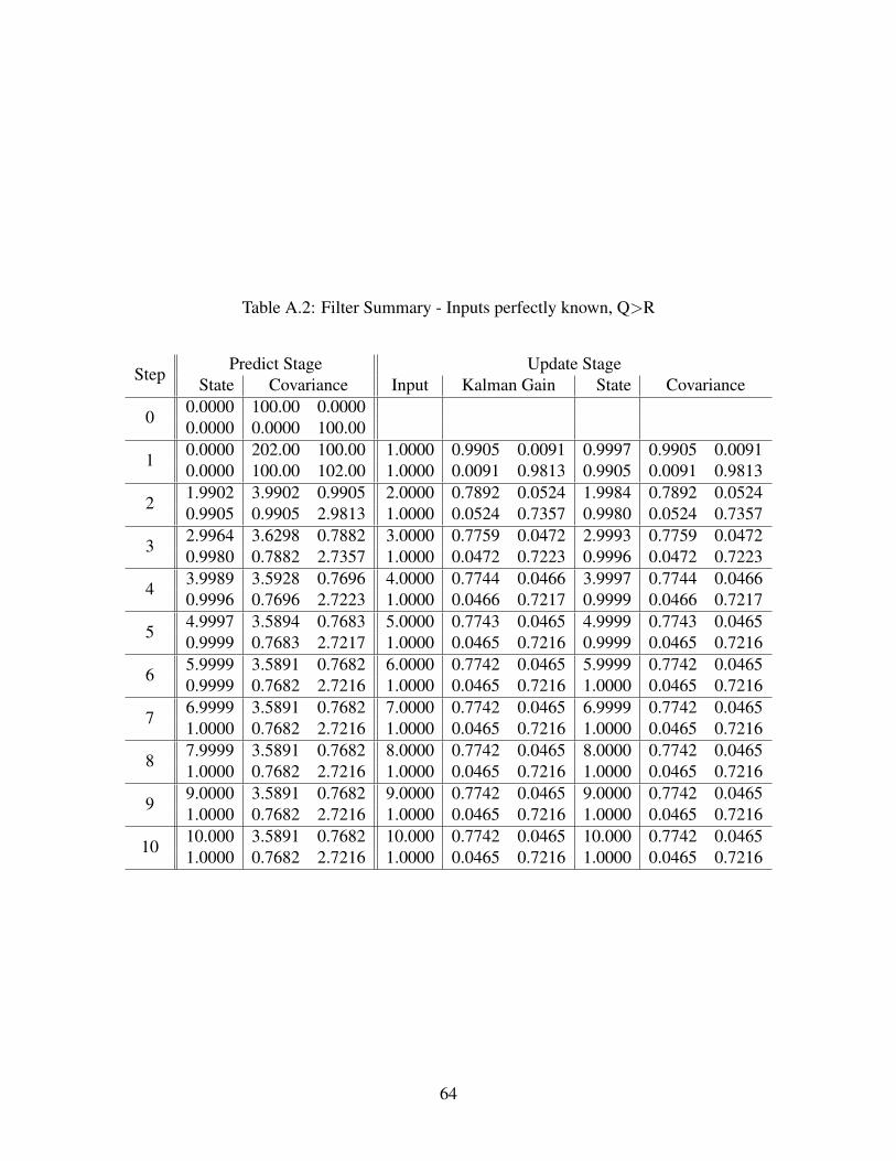
Table A.2: Filter Summary - Inputs perfectly known, Q>R
StepPredict Stage Update Stage
State Covariance Input Kalman Gain State Covariance
00.0000 100.00 0.00000.0000 0.0000 100.00
10.0000 202.00 100.00 1.0000 0.9905 0.0091 0.9997 0.9905 0.00910.0000 100.00 102.00 1.0000 0.0091 0.9813 0.9905 0.0091 0.9813
21.9902 3.9902 0.9905 2.0000 0.7892 0.0524 1.9984 0.7892 0.05240.9905 0.9905 2.9813 1.0000 0.0524 0.7357 0.9980 0.0524 0.7357
32.9964 3.6298 0.7882 3.0000 0.7759 0.0472 2.9993 0.7759 0.04720.9980 0.7882 2.7357 1.0000 0.0472 0.7223 0.9996 0.0472 0.7223
43.9989 3.5928 0.7696 4.0000 0.7744 0.0466 3.9997 0.7744 0.04660.9996 0.7696 2.7223 1.0000 0.0466 0.7217 0.9999 0.0466 0.7217
54.9997 3.5894 0.7683 5.0000 0.7743 0.0465 4.9999 0.7743 0.04650.9999 0.7683 2.7217 1.0000 0.0465 0.7216 0.9999 0.0465 0.7216
65.9999 3.5891 0.7682 6.0000 0.7742 0.0465 5.9999 0.7742 0.04650.9999 0.7682 2.7216 1.0000 0.0465 0.7216 1.0000 0.0465 0.7216
76.9999 3.5891 0.7682 7.0000 0.7742 0.0465 6.9999 0.7742 0.04651.0000 0.7682 2.7216 1.0000 0.0465 0.7216 1.0000 0.0465 0.7216
87.9999 3.5891 0.7682 8.0000 0.7742 0.0465 8.0000 0.7742 0.04651.0000 0.7682 2.7216 1.0000 0.0465 0.7216 1.0000 0.0465 0.7216
99.0000 3.5891 0.7682 9.0000 0.7742 0.0465 9.0000 0.7742 0.04651.0000 0.7682 2.7216 1.0000 0.0465 0.7216 1.0000 0.0465 0.7216
1010.000 3.5891 0.7682 10.000 0.7742 0.0465 10.000 0.7742 0.04651.0000 0.7682 2.7216 1.0000 0.0465 0.7216 1.0000 0.0465 0.7216
64

A.3.3 Q<R, Error = 0
This trial shows what happens when the error is modeled improperly. The measurements areperfect, but the filter sees less uncertainty in the model. For this reason it trusts the prediction overthe measurements and the error converges to zero more slowly.
Q =
[1 00 1
], R =
[3 00 2
], Error = 0%
(a) (b)
Figure A.9: Filter error. Prediction stage error (left) and update stage error (right). The filter erroris in black, the measurement error is in blue.
65

Table A.3: Filter Summary - Inputs perfectly known, Q<R
StepPredict Stage Update Stage
State Covariance Input Kalman Gain State Covariance
00.0000 100.00 0.0000 0.0000 0.0000 0.0000 0.0000 0.0000 0.00000.0000 0.0000 100.00 0.0000 0.0000 0.0000 0.0000 0.0000 0.0000
10.0000 201.00 100.00 1.0000 0.9719 0.0272 0.9991 2.9158 0.05440.0000 100.00 101.00 1.0000 0.0181 0.9629 0.9811 0.0544 1.9258
21.9802 5.9506 1.9803 2.0000 0.6321 0.1479 1.9955 1.8963 0.29580.9811 1.9803 2.9258 1.0000 0.0986 0.5543 0.9935 0.2958 1.1086
32.9890 4.5966 1.4044 3.0000 0.5784 0.1441 2.9963 1.7353 0.28820.9935 1.4044 2.1086 1.0000 0.0960 0.4803 0.9976 0.2882 0.9607
43.9940 4.2725 1.2489 4.0000 0.5638 0.1375 3.9977 1.6916 0.27500.9976 1.2489 1.9607 1.0000 0.0916 0.4661 0.9993 0.2750 0.9322
54.9970 4.1739 1.2073 5.0000 0.5590 0.1353 4.9987 1.6771 0.27070.9993 1.2073 1.9322 1.0000 0.0902 0.4636 0.9999 0.2707 0.9273
65.9986 4.1460 1.1981 6.0000 0.5575 0.1349 5.9994 1.6726 0.26990.9999 1.1981 1.9273 1.0000 0.0899 0.4632 1.0000 0.2699 0.9265
76.9994 4.1391 1.1965 7.0000 0.5571 0.1349 6.9997 1.6714 0.26981.0000 1.1965 1.9265 1.0000 0.0899 0.4632 1.0000 0.2698 0.9264
87.9998 4.1377 1.1963 8.0000 0.5570 0.1349 7.9999 1.6712 0.26991.0000 1.1963 1.9264 1.0000 0.0899 0.4632 1.0000 0.2699 0.9264
98.9999 4.1375 1.1963 9.0000 0.5570 0.1349 8.9999 1.6711 0.26991.0000 1.1963 1.9264 1.0000 0.0899 0.4632 1.0000 0.2699 0.9264
1010.000 4.1374 1.1963 10.000 0.5570 0.1349 10.000 1.6711 0.26991.0000 1.1963 1.9264 1.0000 0.0899 0.4632 1.0000 0.2699 0.9264
66
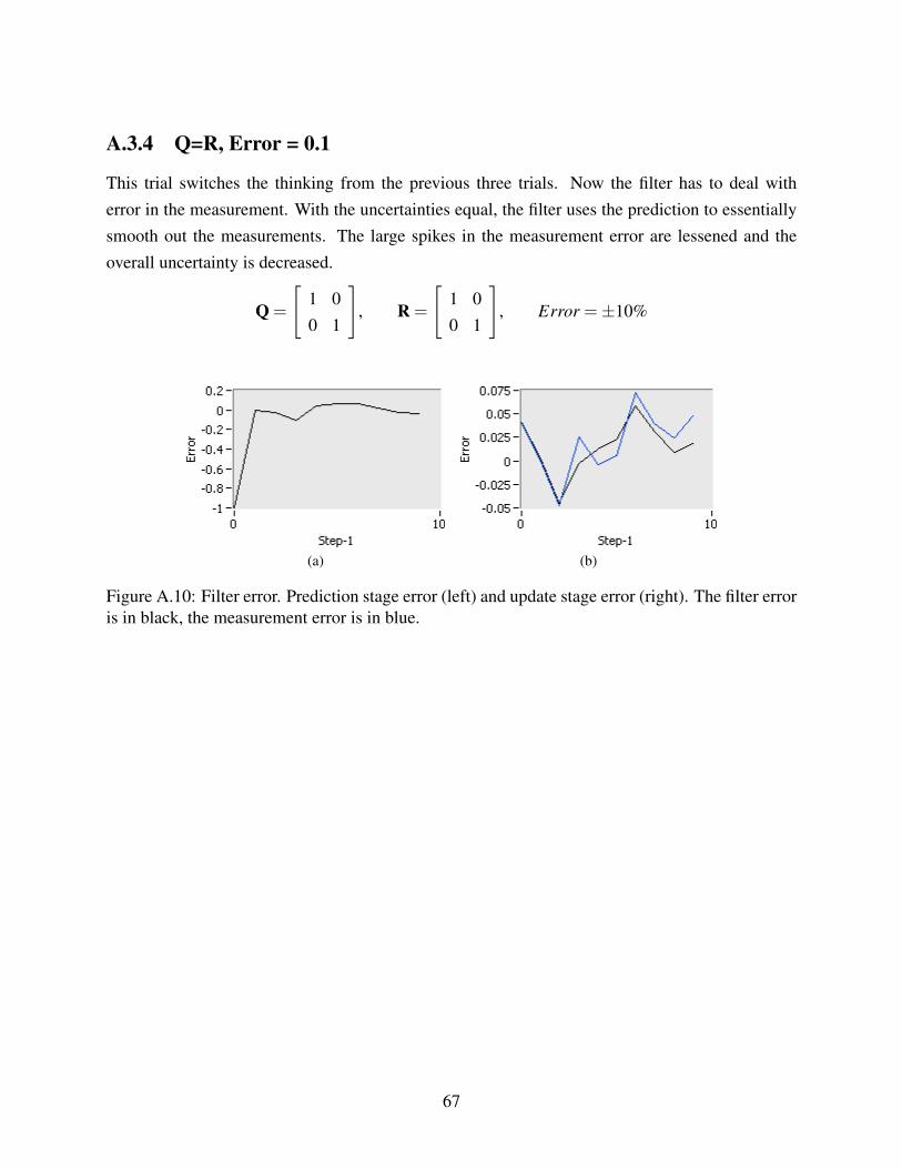
A.3.4 Q=R, Error = 0.1
This trial switches the thinking from the previous three trials. Now the filter has to deal witherror in the measurement. With the uncertainties equal, the filter uses the prediction to essentiallysmooth out the measurements. The large spikes in the measurement error are lessened and theoverall uncertainty is decreased.
Q =
[1 00 1
], R =
[1 00 1
], Error =±10%
(a) (b)
Figure A.10: Filter error. Prediction stage error (left) and update stage error (right). The filter erroris in black, the measurement error is in blue.
67

Table A.4: Filter Summary - Inputs ± 10%, Q=R
StepPredict Stage Update Stage
State Covariance Input Kalman Gain State Covariance
00.0000 100.00 0.0000 0.0000 0.0000 0.0000 0.0000 0.0000 0.00000.0000 0.0000 100.00 0.0000 0.0000 0.0000 0.0000 0.0000 0.0000
10.0000 201.00 100.00 1.0411 0.9903 0.0094 1.0402 0.9903 0.00940.0000 100.00 101.00 0.9701 0.0094 0.9809 0.9614 0.0094 0.9809
22.0017 2.9901 0.9903 2.0006 0.7268 0.0907 2.0027 0.7268 0.09070.9614 0.9903 1.9809 0.9812 0.0907 0.6343 0.9739 0.0907 0.6343
32.9766 2.5427 0.7251 2.9517 0.7008 0.0823 2.9546 0.7008 0.08230.9739 0.7251 1.6343 0.9179 0.0823 0.5977 0.9384 0.0823 0.5977
43.8930 2.4632 0.6800 4.0249 0.6956 0.0796 3.9975 0.6956 0.07960.9384 0.6800 1.5977 1.0983 0.0796 0.5941 1.0439 0.0796 0.5941
55.0415 2.4491 0.6738 4.9957 0.6945 0.0793 5.0119 0.6945 0.07931.0439 0.6738 1.5941 1.0720 0.0793 0.5939 1.0569 0.0793 0.5939
66.0689 2.4471 0.6732 6.0059 0.6944 0.0793 6.0234 0.6944 0.07931.0569 0.6732 1.5939 1.0345 0.0793 0.5938 1.0386 0.0793 0.5938
77.0620 2.4469 0.6732 7.0724 0.6943 0.0793 7.0590 0.6943 0.07931.0386 0.6732 1.5938 0.9093 0.0793 0.5938 0.9626 0.0793 0.5938
88.0217 2.4469 0.6732 8.0391 0.6943 0.0793 8.0307 0.6943 0.07930.9626 0.6732 1.5938 0.9240 0.0793 0.5938 0.9411 0.0793 0.5938
98.9718 2.4469 0.6732 9.0247 0.6943 0.0793 9.0093 0.6943 0.07930.9411 0.6732 1.5938 0.9505 0.0793 0.5938 0.9509 0.0793 0.5938
109.9602 2.4469 0.6732 10.047 0.6943 0.0793 10.018 0.6943 0.07930.9509 0.6732 1.5938 0.9216 0.0793 0.5938 0.9404 0.0793 0.5938
68

A.3.5 Q>R, Error = 0.1
This trial assigns a higher uncertainty to the model. Intuition says that if the predictor is uncertain,trust the measurements more. This is exactly what the filter does.
Q =
[2 00 4
], R =
[1 00 1
], Error =±10%
(a) (b)
Figure A.11: Filter error. Prediction stage error (left) and update stage error (right). The filter erroris in black, the measurement error is in blue.
69

Table A.5: Filter Summary - Inputs ± 10%, Q>R
StepPredict Stage Update Stage
State Covariance Input Kalman Gain State Covariance
00.0000 100.00 0.0000 0.0000 0.0000 0.0000 0.0000 0.0000 0.00000.0000 0.0000 100.00 0.0000 0.0000 0.0000 0.0000 0.0000 0.0000
10.0000 202.00 100.00 0.9290 0.9907 0.0088 0.9285 0.9907 0.00880.0000 100.00 104.00 0.9271 0.0088 0.9820 0.9186 0.0088 0.9820
21.8472 3.9904 0.9908 2.0770 0.7928 0.0343 2.0296 0.7928 0.03430.9186 0.9908 4.9820 0.9241 0.0343 0.8271 0.9310 0.0343 0.8271
32.9606 3.6885 0.8614 2.9668 0.7807 0.0324 2.9649 0.7807 0.03240.9310 0.8614 4.8271 0.9140 0.0324 0.8235 0.9172 0.0324 0.8235
43.8822 3.6691 0.8560 4.0655 0.7798 0.0323 4.0277 0.7798 0.03230.9172 0.8560 4.8235 0.9954 0.0323 0.8235 0.9875 0.0323 0.8235
55.0153 3.6681 0.8558 4.9722 0.7798 0.0323 4.9806 0.7798 0.03230.9875 0.8558 4.8235 0.9555 0.0323 0.8235 0.9598 0.0323 0.8235
65.9404 3.6680 0.8558 6.0084 0.7798 0.0323 5.9960 0.7798 0.03230.9598 0.8558 4.8235 1.0399 0.0323 0.8235 1.0279 0.0323 0.8235
77.0240 3.6680 0.8558 6.9181 0.7798 0.0323 6.9413 0.7798 0.03231.0279 0.8558 4.8235 1.0225 0.0323 0.8235 1.0200 0.0323 0.8235
87.9613 3.6680 0.8558 8.0385 0.7798 0.0323 8.0195 0.7798 0.03231.0200 0.8558 4.8235 0.9578 0.0323 0.8235 0.9713 0.0323 0.8235
98.9908 3.6680 0.8558 8.9455 0.7798 0.0323 8.9582 0.7798 0.03230.9713 0.8558 4.8235 1.0547 0.0323 0.8235 1.0385 0.0323 0.8235
109.9967 3.6680 0.8558 10.054 0.7798 0.0323 10.043 0.7798 0.03231.0385 0.8558 4.8235 1.0779 0.0323 0.8235 1.0728 0.0323 0.8235
70

A.3.6 Q<R, Error = 0.1
This trial would make more sense in the current scheme. The model is an accurate representationof the system, so the errors in the measurements should have more uncertainty associated withthem. With this information, the filter behaves more as would be desired. The relatively largeswings in the measurements are mitigated by the model and the error in the output is less than themeasurements alone.
Q =
[1 00 1
], R =
[5 00 5
], Error =±10%
(a) (b)
Figure A.12: Filter error. Prediction stage error (left) and update stage error (right). The filter erroris in black, the measurement error is in blue.
71

Table A.6: Filter Summary - Inputs ± 10%, Q<R
StepPredict Stage Update Stage
State Covariance Input Kalman Gain State Covariance
00.0000 100.00 0.0000 0.0000 0.0000 0.0000 0.0000 0.0000 0.00000.0000 0.0000 100.00 0.0000 0.0000 0.0000 0.0000 0.0000 0.0000
10.0000 201.00 100.00 1.0295 0.9552 0.0422 1.0232 4.7761 0.21120.0000 100.00 101.00 0.9432 0.0422 0.9129 0.9046 0.2112 4.5648
21.9279 10.763 4.7761 2.0102 0.6324 0.1661 1.9930 3.1623 0.83070.9046 4.7761 5.5648 0.9831 0.1661 0.4516 0.9538 0.8307 2.2581
32.9468 8.0819 3.0888 2.9829 0.5807 0.1568 2.9870 2.9038 0.78400.9538 3.0888 3.2581 1.0766 0.1568 0.3358 1.0007 0.7840 1.6794
43.9878 7.1513 2.4634 4.0811 0.5599 0.1411 4.0368 2.7995 0.70581.0007 2.4634 2.6794 0.9777 0.1411 0.3036 1.0069 0.7058 1.5181
55.0437 6.7293 2.2239 4.9047 0.5483 0.1335 4.9603 2.7419 0.66791.0069 2.2239 2.5181 0.9528 0.1335 0.2954 0.9723 0.6679 1.4770
65.9327 6.5549 2.1450 6.0197 0.5429 0.1311 5.9957 2.7147 0.65560.9723 2.1450 2.4770 1.0926 0.1311 0.2936 1.0191 0.6556 1.4683
77.0148 6.4943 2.1239 7.0786 0.5408 0.1305 7.0347 2.7043 0.65281.0191 2.1239 2.4683 0.9072 0.1305 0.2933 0.9946 0.6528 1.4668
88.0294 6.4769 2.1197 8.0465 0.5402 0.1305 8.0305 2.7011 0.65250.9946 2.1197 2.4668 0.9319 0.1305 0.2933 0.9784 0.6525 1.4666
99.0089 6.4730 2.1192 9.0159 0.5400 0.1305 9.0226 2.7004 0.65260.9784 2.1192 2.4666 1.0545 0.1305 0.2933 1.0017 0.6526 1.4665
1010.024 6.4722 2.1191 10.027 0.5400 0.1305 10.022 2.7002 0.65271.0017 2.1191 2.4665 0.9746 0.1305 0.2932 0.9942 0.6527 1.4664
72

A.3.7 Modeled Q, Modeled R, Error = 0.5
In the previous examples, the uncertainties have been randomly assigned values. These values havea direct effect on the measure of error in the filter, the covariance matrix. In order for this value tohave some useful meaning, the errors in the uncertainty matrices need to correspond to measuresof uncertainties. To test the filter further, the error will be increased to 50% of the measurementunit.
In this example, the model is considered accurate, albeit operating on a potentially inaccuratestate. The uncertainty should therefore be low, but in units that reflect the actual state. The mea-surement uncertainty is given by the sensor that is measuring the state. In this case the standarddeviation of the uncertainty will be assumed to be half of a measurement unit, the same as the errorreported by the sensor.
Q =
[0.1 00 0.1
], R =
[0.25 0
0 0.25
], Error =±50%
Despite the large errors in the measurement, the filter is able to use the model to eliminate someof the variation in the measurement. The standard deviation reported by the filter was less than thatof the sensor, at 0.39 units.
(a) (b)
Figure A.13: Filter error. Prediction stage error (left) and update stage error (right). The filter erroris in black, the measurement error is in blue.
73

Table A.7: Filter Summary - Inputs ± 50%, Q,R Modeled
StepPredict Stage Update Stage
State Covariance Input Kalman Gain State Covariance
00.0000 100.00 0.0000 0.0000 0.0000 0.0000 0.0000 0.0000 0.00000.0000 0.0000 100.00 0.0000 0.0000 0.0000 0.0000 0.0000 0.0000
10.0000 200.10 100.00 0.6472 0.9975 0.0024 0.6478 0.2493 0.00060.0000 100.00 100.10 0.8882 0.0024 0.9950 0.8854 0.0006 0.2487
21.5332 0.5993 0.2493 1.6998 0.6646 0.1396 1.6506 0.1661 0.03490.8854 0.2493 0.3487 0.9333 0.1396 0.5243 0.9338 0.0349 0.1310
32.5845 0.4670 0.1659 3.1963 0.6210 0.1307 3.0127 0.1552 0.03260.9338 0.1659 0.2310 1.3029 0.1307 0.4352 1.1744 0.0326 0.1088
44.1872 0.4294 0.1414 3.9523 0.6068 0.1212 3.9875 0.1517 0.03031.1744 0.1414 0.2088 0.7029 0.1212 0.4177 0.9490 0.0303 0.1044
54.9365 0.4167 0.1347 5.0469 0.6011 0.1182 4.9744 0.1502 0.02950.9490 0.1347 0.2044 0.7077 0.1182 0.4147 0.8619 0.0295 0.1036
65.8363 0.4131 0.1332 5.9560 0.5993 0.1176 5.8720 0.1498 0.02940.8619 0.1332 0.2036 0.5557 0.1176 0.4144 0.7491 0.0294 0.1036
76.6212 0.4122 0.1330 7.4171 0.5988 0.1176 7.1372 0.1497 0.02940.7491 0.1330 0.2036 1.0839 0.1176 0.4143 0.9814 0.0294 0.1035
88.1187 0.4121 0.1329 7.7467 0.5988 0.1176 7.8790 0.1497 0.02940.9814 0.1329 0.2035 0.8375 0.1176 0.4143 0.8780 0.0294 0.1035
98.7571 0.4121 0.1329 9.2871 0.5987 0.1176 9.0615 0.1496 0.02940.8780 0.1329 0.2035 0.7683 0.1176 0.4143 0.8949 0.0294 0.1035
109.9565 0.4121 0.1329 10.163 0.5987 0.1176 10.046 0.1496 0.02940.8949 0.1329 0.2035 0.6084 0.1176 0.4143 0.8005 0.0294 0.1035
74