Granular Matter manuscript No.(will be inserted by the editor)

A local constitutive model with anisotropy for ratchetingunder 2D axial-symmetric isobaric deformation

V. Magnanimo · S. Luding

Accepted: 23.02.2011, Revised: 28.03.2011

Abstract A local constitutive model for anisotropicgranular materials is introduced and applied to isobaric(homogeneous) axial-symmetric deformation. The sim-plified model (in the coordinate system of the bi-axialbox) involves only scalar values for hydrostatic andshear stresses, for the volumetric and shear strains aswell as for the new ingredient, the anisotropy modulus.

The non-linear constitutive evolution equations thatrelate stress and anisotropy to strain are inspired by ob-servations from Discrete Element Method (DEM) sim-ulations. For the sake of simplicity, parameters like thebulk and shear modulus are set to constants, while theshear stress ratio and the anisotropy evolve with differ-ent rates to their critical state limit values when sheardeformations become large.

When applied to isobaric deformation in the bi-axialgeometry, the model shows ratcheting under cyclic load-ing. Fast and slow evolution of anisotropy with strain(relative to the evolution of anisotropy in stress) leadto dilatancy and contractancy, respectively. Further-more, anisotropy acts such that it works “against” thestrain/stress, e.g., a compressive strain builds up anisotropythat creates additional stress acting against further com-pression.

1 Introduction

Dense granular materials show interesting behavior andspecial properties, different from classical fluids or solids[5, 9]. This involves dilatancy, yield stress, history de-

V. Magnanimo, S. Luding

Multi Scale Mechanics (MSM), CTW, UTwente,

POBox 217, 7500 AE Enschede, Netherlands;v.magnanimo@utwente.nl, s.luding@utwente.nl

pendence, as well as ratcheting [1, 2] and anisotropy[6, 13,22–24] – among many others.

If an isotropic granular packing is subject to isotropiccompression the shear stress remains close to zero andthe isotropic stress can be related to the volume fraction[8]. Under shear deformation, the shear stress buildsup until it reaches a yield-limit, as described by clas-sical and more recent models, e.g. [11, 13, 23, 24]. Alsothe anisotropy of the contact network varies, as relatedto the opening and closing of contacts, restructuring,and the creation and destruction of force-chains, as con-firmed by DEM simulations [15, 25]. This is at the ori-gin of the interesting behavior of granular media, butis neglected in many continuum models of particulatematter. Only few theories, see e.g. [2, 7, 15, 18–20, 22]and references therein, involve an anisotropy state vari-able. The influence of the micromechanics on the non-coaxiality of stress, strain and anisotropy of soils is de-scribed e.g. in [24]. This is an essential part of a con-stitutive model for granular matter because it containsthe information how the different modes of deformationhave affected the mechanical state of the system. In thissense, anisotropy is a history variable.

In the following, a recently proposed constitutivemodel [17] is briefly presented and then applied to iso-baric axial-symmetric deformation. The (classical) bulkand shear moduli are constants here, in order to be ableto focus on the effect of anisotropy and the anisotropymaterial parameters exclusively.

2 Model System

In order to keep the model as simple as possible, we re-strict ourselves to bi-axial deformations and the bi-axialorientation of the coordinate system. The bi-axial box

2

is shown schematically in Fig. 1, where the strain in the2−direction is prescribed. Due to the bi-axial geometry(assuming perfectly smooth walls), in the global coordi-nate system one has the strain and the stress with onlydiagonal components that, naturally, are the eigenval-ues of the two coaxial tensors:

[ε] =[ε11 00 ε22

], [σ] =

[σ11 00 σ22

]. (1)

The system is subjected to a constant (isotropic) hy-drostatic stress σ0, to confine the particles. The initialstrain and stress are:

[ε0] =[0 00 0

], [σ0] =

[σ0 00 σ0

]. (2)

Fig. 1 Illustration of the bi-axial model system with prescribed

vertical displacement ε22(t) < 0 and constant isotropic confiningstress σh = (σ11 + σ22)/2 = const. = σ0 < 0.

The sign convention for strain and stress of Ref.[17] is adopted: positive (+) for dilatation/extensionand negative (–) for compression/contraction. There-fore, compressive stresses like σ0 are negative. Whenthe top boundary is moved downwards, ε22 (the pre-scribed strain) will have a negative value whereas ε11,as moving outwards, will be positive.

In general, the strain can be decomposed into an(isotropic) volumetric and a (pure shear) deviatoric part,ε = εV + εD. The isotropic strain is

εV =ε11 + ε22

2

[1 00 1

]=

1D

tr(ε) I = εv I , (3)

with dimensionD = 2, unit tensor I, and volume changetr(ε) = 2εv, invariant with respect to the coordinatesystem chosen. Positive and negative εv correspond tovolume increase and decrease, respectively. Accordingly,the deviatoric strain is:

εD = ε− εV =ε11 − ε22

2

[1 00 −1

]= γ ID , (4)

where γ = ε11−ε222 is the scalar that describes the pure

shear deformation and ID is the traceless unit-deviatorin 2D: The unit-deviator has the eigenvalues, +1 and

–1, with the eigen-directions n(+1) = x1 and n(−1) =x2, where the hats denote unit vectors.

The same decomposition can be applied to the stresstensor σ = σH +σD, and leads to the hydrostatic stress

σH =σ11 + σ22

2

[1 00 1

]=

1D

tr(σ)I = σh I , (5)

and the (pure shear) deviatoric stress

σD = σ − σH =σ11 − σ22

2

[1 00 −1

]= τID , (6)

with the scalar (pure) shear stress τ . According to theirdefinition, both γ and τ can be positive or negative.

Finally, one additional tensor that describes the dif-ference of the material stiffnesses in 1− and 2−directions,can be introduced: the structural anisotropy aD (secondorder), related to the deviatoric fabric or stiffness/acoustictensor. Since in the bi-axial system the anisotropy ori-entation is known, the tensor is fully described by thescalar anisotropy modulus A:

aD = A ID . (7)

This leads to three elastic moduli, i.e., bulk-, shear-,and anisotropy-modulus, respectively,

B =12

[C1111 + C2222 + 2λ

2

],

G = B − λ , and

A =C1111 − C2222

2,

where C1111, C2222 and λ = C1122 are elements of the(rank four) stiffness/acoustic tensor of the system, whichin a general constitutive relation of anisotropic elastic-ity, relates stress and strain increments [17]:

δσ = C : δε+ δσs . (8)

The first term in Eq. (8) is reversible (elastic), whilethe second contains the stress response due to possiblyirreversible changes of structure. Using B, G, and A,one can directly relate isotropic and deviatoric stressand strain [17]:

δσh = 2Bδεv +Aδγ and δτ = Aδεv + 2Gδγ . (9)

In summary, for the bi-axial system, the tensors εD,σD, and aD can be represented by the scalars γ, τ ,and A, respectively, while the orientation is fixed to ID.Change of sign corresponds to reversal of deformation-,stress-, or anisotropy-direction.

As special case the model can describe isotropy, forwhich the equality C1111 = C2222 holds, so that A = 0.Then the second term in the isotropic stress and thefirst term in the deviatoric stress Eqs. (9) vanish.

3

In realistic systems, B will increase (decrease) dueto isotropic compression (extension) [8] and alsoG couldchange due to both isotropic or shear deformation [3].The constitutive models describing this dependence ofbulk and shear moduli on strain are in progress, but areneglected here for the sake of simplicity: Only constantB and G are considered, which is a reasonable assump-tion for isobaric deformations that do not much changethe volume, as will be shown below.

2.1 Model with evolution of anisotropy

When there is anisotropy in the system, a positive A inEqs. (9), in our convention, means that the horizontalstiffness is larger than the vertical (A < 0 implies theopposite).

Discrete Element Method simulations [14, 15] of aninitially isotropic system, with A0 = 0, show that dur-ing deformation anisotropy builds up to a limit Amax.It is also observed that the anisotropy varies only dueto shear strain and practically not due to volumetricstrain. Therefore, the evolution of A is described as:

∂A

∂γ= −βA sign(Amax) (Amax −A) ,

∂A

∂εv= 0 , (10)

with Amax = −Am γ/|γ| = −Am sign(γ), see Ref. [17],with positive maximal anisotropy, Am, i.e., the sign ofAmax is determined by the direction of shear.1 Therate of anisotropy evolution βA determines how fastthe anisotropy changes with strain and thus also itapproaches (exponentially) its maximum for large γ.Starting from an isotropic initial configuration, A0 = 0,the growth is linear for small deformations γ.

2.2 Non-linear stress evolution

It is observed from DEM simulations of (horizontal stresscontrolled) bi-axial deformations [14, 15], that the re-sponse of the system stress is not always linear. Forincreasing strain the stress increments decrease untilthe stress saturates in the critical state regime. In Refs.[14,15], the evolution equation that leads to saturationunder vertical compression, is similar to Eq. (10):

∂sd

∂γ= βs sign(γ) (smax

d − sd) , (11)

1 Assume horizontal compression, which corresponds to

γ/|γ| < 0, that leads to an increase of horizontal stiffness and

thus a positive Amax. Compression in vertical direction leads toa negative Amax – while tension in horizontal or vertical direction

lead to negative and positive Amax, respectively.

where sd is the stress deviator ratio:

sd =σ11 − σ22

(σ11 + σ22)=

τ

σh, (12)

and smaxd = −sm

d γ/|γ| = −smd sign(γ), with positive

maximum deviatoric stress ratio smd .

Starting from here, a phenomenological extension ofthe linear model, as described in Eqs. (9), was proposedin Ref. [17], leading to the non-linear, incremental con-stitutive relations:

δσh = 2Bδεv +ASδγ , (13)

δτ = Aδεv + 2GSδγ , and (14)

δA = βA sign(γ) (Amax −A) δγ , (15)

where the stress isotropy S = (1−sd/smaxd ) has been in-

troduced. This quantity characterizes the stress-aniso-tropy in the material, varying between 0 (maximallyanisotropic in strain direction), 1 (fully isotropic) up to2 (maximally anisotropic, perpendicular to the momen-tary strain increment).

Note that, the use of an evolution (or rate-type)equation for the stress, allows for irreversibility in theconstitutive model due to the terms with S only. Suchan approach is similar to hypoplasticity [13] or GSH [11]and differs from elasto-plastic models. In the formerboth elastic and plastic strains always coexist [2].

In summary, besides the five local field variables,σh, τ , εv, γ, and A, the model has only five materialparameters: the bulk and shear moduliB,G, the macro-scopic coefficient of friction, sm

d , the evolution rate ofanisotropy, βA, and the maximal anisotropy Am. Withinitial conditions σ0, S0 = 1−τ0/(σ0s

maxd ), and A0, the

model can be integrated from εv0 = 0 and γ0 = 0.

3 Results

In this section the proposed constitutive model will beused to describe the behavior of a granular materialwhen an isobaric axially symmetric compression (ex-tension) is applied (Sec. 3.1). Vertical compression andextension are then combined in Sec. 3.2 to analyze theresponse of the material to cyclic loading.

Due to the isobaric stress control, the first equationof the constitutive model, Eq. (13), simplifies to:

0 = 2Bδεv +ASδγ . (16)

Different parameters are varied with the goal to under-stand their meaning in the model. We chose the rangeof parameter values roughly referring to soil mechanicsand granular materials experiments [3,12]. In all exam-ples the confining pressure is set to σ0 = −100kPa, the

4

bulk modulus B = 200MPa is set constant, whereas forthe shear modulus four values are used, G = 25, 50, 75,and 100 MPa, corresponding to the dimensionless ratiosG/B = 1/8, 2/8, 3/8, and 4/8, respectively.

The samples are initially isotropic (in stress, S0 = 0,and structure, A0 = 0) and the maximal anisotropy de-pends on the bulk modulus such that Am = B/2. Thedependence of the model on the anisotropy evolutionrate parameter βA is tested. For βA = 0 one recoversthe special case of isotropy (A = A0 = 0). Anisotropicmaterials with different rate of evolution of anisotropy,display several important features of granular matterbehavior. The parameter, sm

d = 0.4 is also chosen fromnumerical simulations with a reasonable contact coeffi-cient of friction µ ≈ 0.5 [14,15].

3.1 Axially symmetric isobaric compression

We study the evolution of anisotropyA, deviatoric stressratio and volume, for vertical compression, (i.e., for pos-itive γ) with constant anisotropy evolution rate βA anddifferent shear moduli G. Since the evolution of A, seeEq. (15), is not affected by G, we do not show it here,but refer to Fig. 3(a) below. For the chosen set of pa-rameters, the anisotropy reaches its (negative) extremevalue within about 0.1% of strain, where the sign indi-cates the fact that the stiffness in vertical (compression)direction is larger than in horizontal (extension) direc-tion.

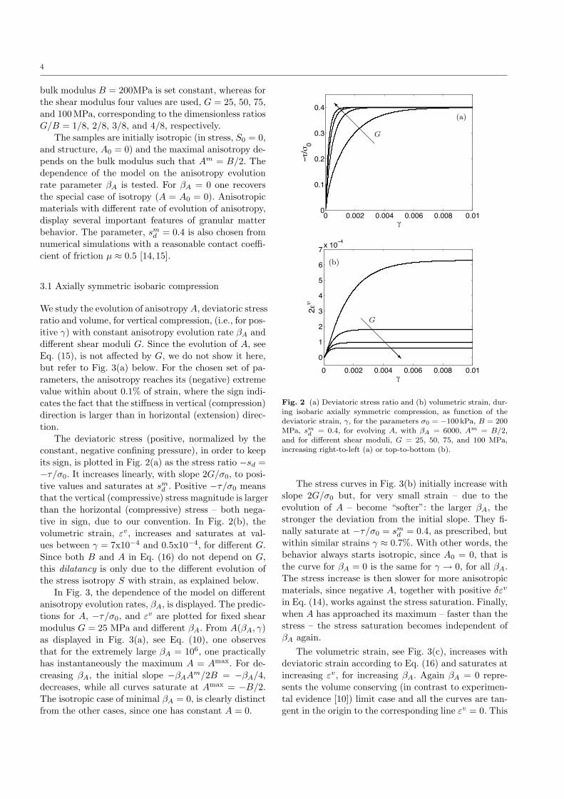
The deviatoric stress (positive, normalized by theconstant, negative confining pressure), in order to keepits sign, is plotted in Fig. 2(a) as the stress ratio −sd =−τ/σ0. It increases linearly, with slope 2G/σ0, to posi-tive values and saturates at sm

d . Positive −τ/σ0 meansthat the vertical (compressive) stress magnitude is largerthan the horizontal (compressive) stress – both nega-tive in sign, due to our convention. In Fig. 2(b), thevolumetric strain, εv, increases and saturates at val-ues between γ = 7x10−4 and 0.5x10−4, for different G.Since both B and A in Eq. (16) do not depend on G,this dilatancy is only due to the different evolution ofthe stress isotropy S with strain, as explained below.

In Fig. 3, the dependence of the model on differentanisotropy evolution rates, βA, is displayed. The predic-tions for A, −τ/σ0, and εv are plotted for fixed shearmodulus G = 25 MPa and different βA. From A(βA, γ)as displayed in Fig. 3(a), see Eq. (10), one observesthat for the extremely large βA = 106, one practicallyhas instantaneously the maximum A = Amax. For de-creasing βA, the initial slope −βAA

m/2B = −βA/4,decreases, while all curves saturate at Amax = −B/2.The isotropic case of minimal βA = 0, is clearly distinctfrom the other cases, since one has constant A = 0.

0 0.002 0.004 0.006 0.008 0.010

0.1

0.2

0.3

0.4

γ

−τ/σ0

(a)

@@

@@@I

G

0 0.002 0.004 0.006 0.008 0.01

0

1

2

3

4

5

6

7x 10

−4

γ

2ευ

(b)

@@@@@R

G

Fig. 2 (a) Deviatoric stress ratio and (b) volumetric strain, dur-

ing isobaric axially symmetric compression, as function of thedeviatoric strain, γ, for the parameters σ0 = −100 kPa, B = 200

MPa, smd = 0.4, for evolving A, with βA = 6000, Am = B/2,

and for different shear moduli, G = 25, 50, 75, and 100 MPa,increasing right-to-left (a) or top-to-bottom (b).

The stress curves in Fig. 3(b) initially increase withslope 2G/σ0 but, for very small strain – due to theevolution of A – become “softer”: the larger βA, thestronger the deviation from the initial slope. They fi-nally saturate at −τ/σ0 = sm

d = 0.4, as prescribed, butwithin similar strains γ ≈ 0.7%. With other words, thebehavior always starts isotropic, since A0 = 0, that isthe curve for βA = 0 is the same for γ → 0, for all βA.The stress increase is then slower for more anisotropicmaterials, since negative A, together with positive δεv

in Eq. (14), works against the stress saturation. Finally,when A has approached its maximum – faster than thestress – the stress saturation becomes independent ofβA again.

The volumetric strain, see Fig. 3(c), increases withdeviatoric strain according to Eq. (16) and saturates atincreasing εv, for increasing βA. Again βA = 0 repre-sents the volume conserving (in contrast to experimen-tal evidence [10]) limit case and all the curves are tan-gent in the origin to the corresponding line εv = 0. This

5

0 0.002 0.004 0.006 0.008 0.01

−0.25

−0.2

−0.15

−0.1

−0.05

0

γ

A/2B

(a)

βA = 0

βA = 106

0 0.002 0.004 0.006 0.008 0.010

0.1

0.2

0.3

0.4

γ

−τ/σ0

0 1 2 3 4

x 10−4

0

0.05

0.1

0.15

0.2

γ

−τ/σ

0

(b)βA = 0

βA = 106

0 0.002 0.004 0.006 0.008 0.01

0

2

4

6

8

x 10−4

γ

2ευ

(c)βA = 106

βA = 0

Fig. 3 (a) Anisotropy, (b) deviatoric stress ratio, and (c) volu-

metric strain during isobaric axially symmetric deformation, asfunction of deviatoric strain, γ, with σ0 = −100 kPa, B = 200MPa and G = 25 MPa, for evolving A, with Am = B/2 andvarying βA, increasing from 0 to 6000 in steps of 1000, from topto bottom in panels (a) and (b), and from bottom to top in panel

(c). The inset in (b) is a zoom into the small strain response. The

green-dashed and red-solid lines represent the extreme cases ofisotropy βA = 0, (A = 0) and constant, instantaneous maximal

anisotropy, βA = 106, (A = Amax), respectively.

is due to Eq. (16), where A = 0, for isobaric axially sym-metric compression, leads to δεv = −ASδγ/2B = 0.With purely deviatoric strain, volumetric strain cannot exist without anisotropy. Nevertheless, the isotropic

case A0 = 0 can be a proper description of the incre-mental response of an initially isotropic granular ma-terial, when very small strains are applied (consistentwith experimental observations).

Similar results (besides different signs) are obtainedwhen an axially symmetric vertical extension with con-stant pressure is applied.

3.2 Strain reversal

Now vertical compression and extension are combined,resembling cyclic loading. The path is strain-controlled,that is the strain increment is reversed after a certainshear strain is accumulated. We start with compression,until about 1% of vertical integrated strain, ε22 ' 0.01,is reached, ensuring the system to be in the well es-tablished critical state flow regime (for large βA). Af-ter reversal vertical extension is carried on until it alsoreaches 1%, relative to the original configuration. Atthis point the increment is reversed again and a newcompression-extension cycle starts.

In particular, we want to understand how the rate ofanisotropy evolution influences the cyclic loading path.For fixed shear (and bulk) modulus, we compare the be-havior for two different values of βA. Figs. 4(a,c,e,g) and4(b,d,f,h) show the system properties as functions ofthe deviatoric strain, γ, for anisotropy rates βA = 2000and 400, respectively. For both anisotropy (a,b) andstress-ratio (c,d), except for the first loading, this re-lation consists of hysteresis loops of constant width asconsecutive load-unload cycles are applied. This hys-teresis produces an accumulation of both isotropic anddeviatoric strain, positive for large βA and negative forsmall βA, see Figs. 4(e,f). Figures 4(c) and 4(d) showthat the deviatoric stress increases due to compression,until load reversal (extension) and decreases to nega-tive values until the next reversal. Under load rever-sal, the corresponding stress response is realized withidentical loading and un-loading stiffnesses. In agree-ment with Fig. 3(b), anisotropy decreases (increases)faster for larger βA, whereas the stress ratio τ/σ0 ap-proaches its maximum somewhat slower, due to the op-posite signs of the two terms on the r.h.s. in Eq. (14).

In Figs. 4(e) and 4(f), the accumulation of small per-manent deformations, after each cycle, both isotropicand deviatoric, are displayed. Overall, the ratchetingleads to an increase (decrease) of volume in each cy-cle for large (small) βA, respectively. The sign-reversalof the anisotropy modulus A during each half-cycle isresponsible for the sign of the volumetric strain. Thiscomes directly from the analysis of Eq. (16): the stressisotropy S can only be positive and A changes signwith increasing deviatoric strain γ, after each reversal.

6

−0.015 −0.01 −0.005 0 0.005 0.01 0.015

−0.2

−0.1

0

0.1

0.2

0.3

γ

A/2B

−0.015 −0.01 −0.005 0 0.005 0.01 0.015

−0.2

−0.1

0

0.1

0.2

0.3

γ

A/2B

(a) (b)

- �

−0.015 −0.01 −0.005 0 0.005 0.01

−0.4

−0.2

0

0.2

0.4

γ

−τ/σ0

−0.015 −0.01 −0.005 0 0.005 0.01

−0.4

−0.2

0

0.2

0.4

γ

−τ/σ0

(c) (d)

- �

−0.015 −0.01 −0.005 0 0.005 0.01 0.0150

1

2

3

4

5

6x 10

−3

γ

2ευ

−0.015 −0.01 −0.005 0 0.005 0.01 0.015−5

−4

−3

−2

−1

0

1x 10

−3

γ

2ευ

(e)

•01

3

5

7

9

(f)•

01

3

5

7

9

-

-

0 0.005 0.01 0.015

−0.5

−0.4

−0.3

−0.2

−0.1

0

0.1

0.2

γ

AS/2B

0 0.005 0.01 0.015

−0.5

−0.4

−0.3

−0.2

−0.1

0

0.1

0.2

γ

AS/2B

(g)

0

13579

(h)

0

13579

-

?

���

-

-

?

�

Fig. 4 Anisotropy, A/2B (a, b), deviatoric stress, −τ/σ0 (c, d), volumetric strain, 2εv (e, f), and the contractancy/dilatancy ratioAS/2B (g, h), during isobaric axially symmetric deformation and cyclic loading, with σ0 = −100 kPa, G = 25MPa and B = 200MPa,

for evolving A, Am = B/2, βA = 2000 (Left) and βA = 400 (Right).

7

The volumetric strain accumulates monotonically fol-lowing the behavior of A. Interestingly, βA, the rate ofchange of A, controls the net volume change. The orig-inal reason for this behavior becomes clear looking atFigs. 4(g) and 4(h), where the variation of the contrac-tancy/dilatancy ratio AS/2B (during initial loading (0)and the odd reversal points (1, 3, 5, 7, 9)) is shown forthe two different βA. At the beginning (0), the quantitybecomes always negative due to the initial decrease ofA: that is, the system always shows initial dilatancy,see path 0 − 1 in 4(e) and 4(f). Only after the firstreversal the influence of βA on dilatancy/compactancyshows up. This initial part of the cyclic loading corre-sponds to what is discussed in Fig. 2. The integrationof AS/2B over γ leads to increasing εv in the first case(g) and decreasing εv in the second (h). Rapid changesof the anisotropy modulus A, corresponding to largeβA, lead to dilation, whereas slow changes of A lead tocompaction.

Besides the trivial case of anisotropy rate βA = 0,the analysis leads to the existence of a second value ofβc

A such that there is no volume change in the material,as shown in Fig. 5(a). The second material parameterin Eq. (10), the maximal anisotropy Am, also influencesratcheting. For all Am studied, the volume change percycle rapidly drops and then increases with βA, reachinglarger values for larger Am. The critical βc

A, correspond-ing to no volume change, decreases with Am increasing.The amount of strain accumulation per cycle, ∆εv, andβc

A also depend on the shear modulus G, see Fig. 5(b).In fact, larger G leads to a faster increase of the stressdeviator ratio sd, that is a faster decrease of the stressisotropy S in Eq. (16). Moreover, the critical value βc

A

increases when the shear modulus increases.

The behavior reported in Figs. 4(e) and 4(f) is quali-tatively in agreement with physical experiments. Strainaccumulation appears, when a granular sample is sub-jected to simple-shear stress reversals in a triaxial cellwith constant radial stress [21] or in a torsional resonantcolumn with constant mean-stress [4]. Interestingly, thebehavior of the material is shown to be amplitude de-pendent [21]. The model is able to reproduce such a de-pendence and the strain accumulation vanishes for verysmall amplitude (data not shown). The un-physical con-stant accumulation per cycle, see Fig. 4(e) and (f), inour opinion, will disappear when evolution laws for Band G are considered. An accurate comparison withexperimental and numerical data is subject of a futurestudy.

102

103

104

−5

0

5

10

15x 10

−3

log(βA)

∆(2ευ

)

(a)

0 0.2 0.4 0.6 0.8 1

0

1

2

3

4 x 10 3

G/B

(2)

(b)

10 1 10010 7

10 6

10 5

10 4

10 3

10 2

slope= −2

Fig. 5 Strain accumulation per cycle ∆(2εv) with σ0 =−100 kPa and B = 200MPa for evolving A. In panel (a) ∆(2εv)

is plotted against log(βA) with Am = 2B/3 (red dashed line),

Am = B/2 (black solid line), Am = 2B/5 (green dotted line)and fixed G = 25MPa. In panel (b) ∆(2εv) is plotted against

G/B, with fixed βA = 6000; in the inset the same quantities are

plotted in logarithmic scale.

4 Summary and Conclusion

In the bi-axial system – where the eigen-vectors of alltensors are either horizontal or vertical – a new consti-tutive model, as inspired by DEM simulations in Ref.[14, 15], is presented in Eqs. (13), (14), and (15). Itinvolves incremental evolution equations for the hydro-static and deviatoric stresses and for the single (struc-tural) anisotropy modulus that varies differently fromthe stress-anisotropy during deviatoric deformations ofthe system and thus represents a history/memory pa-rameter [17]. The five local field variables are σh, τ , εv,γ, and A.

The model involves only three moduli: the classi-cal bulk modulus, B, the shear modulus, G, and theanisotropy modulus, A, whose sign indicates the direc-tion of anisotropy in the present formulation. Due to theanisotropy, A, the model involves a cross coupling of thetwo types of strains and stresses, namely isotropic andshear (deviatoric). As opposed to isotropic materials,shear strain can cause e.g. dilation and hence compres-

8

sive stresses. Similarly, a purely volumetric strain cancause shear stresses and thus shear deformation in thesystem. As main hypothesis, the anisotropy evolution iscontrolled by the anisotropy rate βA and by deviatoricstrain, γ, but not (directly) by stress.

The model also leads to a critical state regime, wherethe volume, the stresses, and the anisotropy modulus donot change anymore. The critical state is described bythe maximal anisotropy Am and the maximal deviatoricstress ratio sm

d , equivalent to a macroscopic friction co-efficient [16].

To better understand the model, a series of simu-lations has been performed for special cases. For verysmall strains, linear relations between stresses and strainsare observed, while for larger strains the non-linear be-havior sets in with a particular cross-coupling betweenisotropic and deviatoric components through both stress-ratio, sd, and structure-anisotropy, A – leading to non-linear response at load-reversal. Dilation or compactionafter large amplitude cyclic load reversal are related tofast or slow evolution of the anisotropy, A, respectively.

Comparison with DEM simulations is in progress.The next step is the formulation of the model for arbi-trary orientations of the stress-, strain- and anisotropy-tensors, but keeping the number of parameters fixed.This will eventually allow, e.g., a Finite Element Methodimplementation, in order to study arbitrary boundaryconditions other than homogeneous bi-axial systems.Furthermore, the model will be generalized to three di-mensions in the spirit of Ref. [17], where (at least) onemore additional anisotropy parameter (tensor) is ex-pected to be present in arbitrary deformation histories.

Acknowledgements This work is dedicated to late Prof. I. Var-

doulakis and his inspiring publications. Helpful discussions with

J. Goddard, D. Krijgsman, M. Liu, S. McNamara, E. S. Per-dahcıoglu, A. Singh, S. Srivastava, H. Steeb, J. Sun and S. Sun-

daresan are gratefully acknowledged. The work was financially

supported by an NWO-STW VICI grant.

References

1. F. Alonso-Marroquin and H. J. Herrmann. Ratcheting ofgranular materials. Phys. Rev. Lett., 92(5), 2004.

2. F. Alonso-Marroquin, S. Luding, H. J. Herrmann, and I. Var-

doulakis. Role of anisotropy in the elastoplastic response ofa polygonal packing. Phys. Rev. E, 71:051304–(1–18), 2005.

3. Y. Chen, I. Ishibashi, and J. Jenkins. Dynamic shear mod-

ulus and fabric: part I, depositional and induced anisotropy.Geotechnique, 1(38):25–32, 1988.

4. Y. Chen, I. Ishibashi, and J. Jenkins. Dynamic shear modulus

and fabric: part II, stress reversal. Geotechnique, 1(38):33–37, 1988.

5. P. G. de Gennes. Granular matter: a tentative view. Reviews

of Modern Physics, 71(2):374–382, 1999.

6. L. Geng, G. Reydellet, E. Clement, and R. P. Behringer.

Green’s function measurements in 2D granular materials.

Physica D, 182:274–303, 2003.7. J. Goddard. Granular hypoplasticity with Cosserat effects. In

J. Goddard, P. Giovine, and J. T. Jenkins, editors, IUTAM-

ISIMM Symposium on Mathematical Modeling and PhysicalInstances of Granular Flows, pages 323–332, Reggio Calabria

(Italy), 14-18 September 2009, 2010. AIP.

8. F. Goncu, O. Duran, and S. Luding. Constitutive rela-tions for the isotropic deformation of frictionless packings of

polydisperse spheres. C. R. Mecanique, 338(10-11):570–586,

2010.9. H. M. Jaeger, S. R. Nagel, and R. P. Behringer. Granular

solids, liquids, and gases. Rev. Mod. Phys., 68(4):1259–1273,1996.

10. J. Jenkins, P. Cundall, and I. Ishibashi. Micromechanical

modeling of granular materials with the assistance of exper-iments and numerical simulations. In Biarez and Gourves,

editors, Powders and Grains, pages 257– 264, Rotterdam,

1989. Balkema.11. Y. Jiang and M. Liu. Granular solid hydrodynamics. Gran-

ular Matter, 11(3):139–156, 2009.

12. Y. Khidas and X. Jia. Anisotropic nonlinear elasticity in aspherical-bead pack: Influence of the fabric anisotropy. Phys.

Rev. E, 81:21303, Feb 2010.

13. D. Kolymbas. An outline of hypoplasticity. Arch. App.Mech., 61:143–154, 1991.

14. S. Luding. Micro-macro models for anisotropic granular me-dia. In P. A. Vermeer, W. Ehlers, H. J. Herrmann, and

E. Ramm, editors, Modelling of Cohesive-Frictional Mate-

rials, pages 195–206, Leiden, Netherlands, 2004. Balkema.15. S. Luding. Anisotropy in cohesive, frictional granular media.

J. Phys.: Condens. Matter, 17:S2623–S2640, 2005.

16. S. Luding and F. Alonso-Marroquin. The critical-state yieldstress (termination locus) of adhesive powders from a single

numerical experimen. Granular Matter, 13(2):109–119, 2011.

17. S. Luding and S. Perdahcioglu. A local constitutive modelwith anisotropy for various homogeneous 2d biaxial deforma-

tion modes. CIT, DOI: 10.1002/cite.201000180, 2011.

18. H. Muhlhaus, L. Moresi, L. Gross, and J. Grotowski. The in-fluence of non-coaxiality on shear banding in viscous-plastic

materials. Granular Matter, 12:229–238, 2010.19. J. Sun and S. Sundaresan. A plasticity model with mi-

crostructure evolution for quasi-static granular flows. In

J. Goddard, P. Giovine, and J. T. Jenkins, editors, IUTAM-ISIMM Symposium on Mathematical Modeling and Physical

Instances of Granular Flows, pages 280–289, Reggio Calabria

(Italy), 14-18 September 2009, 2010. AIP.20. J. Sun and S. Sundaresan. A plasticity model with mi-

crostructure evolution for quasi-static granular flows. J.

Fluid Mech., submitted, 2010.21. F. Tatsuoka and K. Ishihara. Drained deformation of sand

under cyclic stresses reversing direction. Soils and founda-

tion, 3(14):51–65, 1974.22. J. Tejchman, E. Bauer, and W. Wu. Effect of fabric

anisotropy on shear localization in sand during plane straincompression. Acta Mechanica, 189:23–51, 2007.

23. I. Vardoulakis and G. Frantziskonis. Micro-structure inkinematic-hardening plasticity. European Journal of Me-chanics A-Solids, 11(4):467, 1992.

24. I. Vardoulakis and J. Sulem. Bifurcation analysis in geome-

chanics. Chapman & Hall, London, 1995.25. J. Zhang, T. S. Majmudar, A. Tordesillas, and R. P.

Behringer. Statistical properties of a 2D granular material

subjected to cyclic shear. Granular Matter, 12:159–172, 2010.