A Linear Logic Model of State

Uday S. Reddy

Department of Computer ScienceUniversity of Illinois at Urbana-Champaign

Urbana, IL 61801Net: reddy@cs.uiuc.edu

Janurary 8, 1993

Abstract

We propose an abstract formal model of state manipulation in the framework ofGirard’s linear logic. Two issues motivate this work: how to describe the semantics ofhigher-order imperative programming languages and how to incorporate state manipu-lation in functional programming languages. The central idea is that a state is linearand “regenerative”, where the latter is the property of a value that generates a new valueupon each use. Based on this, we define a type constructor for states and a “modality”type constructor for regenerative values. Just as Girard’s “of course” modality allowshim to express static values and intuitionistic logic within the framework of linear logic,our regenerative modality allows us to express dynamic values and imperative programswithin the same framework. We demonstrate the expressiveness of the model by showingthat a higher-order Algol-like language can be embedded in it.

1 Introduction

Programming in the real world typically involves state-manipulation. All the major pro-gramming languages widely in use, except for “pure functional” languages like Haskell,support variables and assignments. A large number of programming applications rangingfrom window managers to process control systems involve the manipulation of state. Unfor-tunately, there are relatively few mathematical tools available to the programmer to reasonabout such programs and applications. The object of this paper to propose a model ofstate inspired by linear logic, which can serve as the foundation for building mathematicaltheories of state manipulation.

Linear logic has, from the beginning, evoked ideas of state. Girard [Gir87b] and La-font [Laf88] give example applications for modelling state via linearity. Wadler has explicitlyproposed linearity as a means for representing state in functional languages [Wad90, Wad91].However, one finds that many aspects of state-manipulation are not modelled by theseproposals. How does one model the identity of a history-sensitive object which persists overa period of time and supports operations for its use? How does one model sequencing? Howdoes one model hierarchical abstractions where new objects are constructed from existingobjects?

1

To build a model of state using linear logic ideas, we found it necessary to make twoextensions to linear logic. One is a binary connective called “before” which was alreadyproposed by Girard, and studied extensively in Retore’s dissertation [Ret93b]. The secondis a “regenerative” storage operator (or modality) which stands in the same relation to“before” as the “of course” operator does to tensor. By extending intuitionistic linear logicwith these two constructions, we obtain a logical system dubbed the “linear logic model ofstate”.

While our own intuitions are derived from this logical system, for pedagogical clarity, wepresent its semantics first. In Section 2, we define the two constructions in the context ofcoherent spaces. Section 3 is a semantical study of the Kleisli category of the regenerativestorage operator. We show that the maps of this category correspond to identifiableclasses of functions. Next, we show that these constructions model state-manipulationby interpreting a fragment of Algol using them (Section 4). Finally, we present the logicalsystem itself in Section 5.

2 Two Constructions in Coherent Spaces

For modelling state and sequential computations, we need two constructions in addition tothose of linear logic. The first is a binary connective called “before” (written “>”) whichdenotes sequential composition of components. The second is a “regenerative” storageoperator (written “†”) which allows us to build sequentially reusable storage objects. Inthis section, we use the framework of Girard’s coherent spaces [GLT89, Gir87a] to giveconcrete semantic intuitions about these constructions.

We assume a general familiarity with coherent spaces. See [GLT89, Chaps. 8 and 12]for basic notions and [Gir87a, Sec. 3] for coherent semantics of linear logic. (We refer tothe “classical” features of this semantics for pedagogical reasons even though they are notessential for the model of state presented here. A reader is comfortable with intuitionisticlinear logic may consult Appendix A for a quick review of the classical features.) Wealso mention various categorical facts in the passing. See [Mac71, Laf88, See89, Jac92] fordefinitions. First, recall the basic definition of coherent spaces.

2.1 Definition A coherent space is a pair A = (|A|, _A) where• |A| is a set, whose members are called tokens, and• _

A is a binary reflexive relation on |A|, called coherence.We write α _

A α′ as α _ α′ [mod A] for convenience (or just α _ α′, depending oncontext). Define notations:

(strict coherence) α _ α′ [modA] ⇐⇒ α _ α′ [modA] ∧ α 6= α′

(strict incoherence) α ^ α′ [modA] ⇐⇒ ¬α _ α′ [modA](incoherence) α � α′ [modA] ⇐⇒ α ^ α′ [modA] ∨ α = α′

⇐⇒ ¬α _ α′ [modA]

A linear map F : A −◦ B is a subset of |A| × |B| such that, for all (α, β), (α′ , β′) ∈ F ,

α _ α′ ⇒ β _ β′ ∧ α _ α′ ⇒ β _ β′

2

Coherent spaces and linear maps form a category COHL.An element (or point) of A is a coherent set in A, i.e., a subset a ⊆ |A| such that, for all

α, α′ ∈ a, α _ α′ [modA]. The elements of A form an atomic Scott domain under inclusionorder.1 We denote this domain by D(A).2 A liner map F : A −◦ B determines a functionf : D(A) → D(B) given by f(a) = {β : ∃α ∈ a. (α, β) ∈ F }. The function f is stable, i.e.,preserves meets of pairs of compatible elements:

x ↑ y =⇒ f(x u y) = f(x) u f(y) (1)

and linear, i.e., preserves the lubs of bounded sets:

S ↑ =⇒ f(⊔S) =

⊔f(S) (2)

Henceforth, we will call linear, stable functions simply “linear functions”. Note that a linearfunction is continuous and strict. Conversely, given a linear function f : D(A) → D(B), wecan recover F (called the trace of f) by

F = { (α, β) : α ∈ |A|, β ∈ f({α}) }.

It can be shown that the category COHL is equivalent to the category of atomic Scottdomains and linear functions.

We call a linear map a linear injection if its underlying relation f ⊆ |A| × |B| is aninjection. Linear injections are monomorphisms in COHL (among others).

Before

2.2 Recall the connectives ⊗ and............................................................................................... :

|A⊗B| = |A| × |B|(α, β) _ (α′, β′) [modA⊗B] ⇐⇒ α _ α′ [modA] ∧ β _ β′ [modB]

|A............................................................................................... B| = |A| × |B|(α, β) _ (α′, β′) [modA

............................................................................................... B] ⇐⇒ α _ α′ [modA] ∨ β _ β ′ [modB]

Notice that

(α, β) _ (α′, β′) [modA⊗B] =⇒ (α, β) _ (α′, β′) [modA............................................................................................... B]

(α, β) _ (α′, β′) [modA⊗B] =⇒ (α, β) _ (α′, β′) [modA............................................................................................... B]

This implies a linear injection mix : A⊗B −◦ A............................................................................................... B.

2.3 We can now postulate another connective > (“before”) with linear injections:

A⊗B −◦ A >B −◦ A............................................................................................... B.

1An atom is an element x such that x′ v x implies x′ = ⊥∨x′ = x. A domain is atomic if every elementis the lub of the set of atoms below it.

2Girard [GLT89] calls D(A) a coherent space and calls A the web of the coherent space.

3

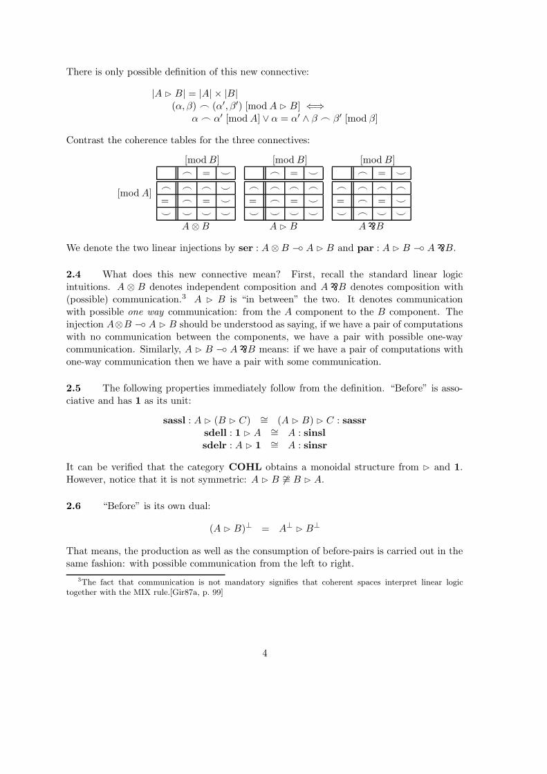
There is only possible definition of this new connective:

|A B B| = |A| × |B|(α, β) _ (α′, β′) [modA B B] ⇐⇒

α _ α′ [modA] ∨ α = α′ ∧ β _ β′ [mod β]

Contrast the coherence tables for the three connectives:

[modA]

[modB]

_ = ^

_ _ _ ^

= _ = ^

^ ^ ^ ^

[modB]

_ = ^

_ _ _ _

= _ = ^

^ ^ ^ ^

[modB]

_ = ^

_ _ _ _

= _ = ^

^ _ ^ ^

A⊗B A B B A............................................................................................... B

We denote the two linear injections by ser : A⊗B −◦ A B B and par : A B B −◦ A............................................................................................... B.

2.4 What does this new connective mean? First, recall the standard linear logicintuitions. A ⊗ B denotes independent composition and A

............................................................................................... B denotes composition with

(possible) communication.3 A B B is “in between” the two. It denotes communicationwith possible one way communication: from the A component to the B component. Theinjection A⊗B −◦ A B B should be understood as saying, if we have a pair of computationswith no communication between the components, we have a pair with possible one-waycommunication. Similarly, A B B −◦ A

............................................................................................... B means: if we have a pair of computations with

one-way communication then we have a pair with some communication.

2.5 The following properties immediately follow from the definition. “Before” is asso-ciative and has 1 as its unit:

sassl : A B (B B C) ∼= (A B B) B C : sassrsdell : 1 B A ∼= A : sinsl

sdelr : A B 1 ∼= A : sinsr

It can be verified that the category COHL obtains a monoidal structure from B and 1.However, notice that it is not symmetric: A B B 6∼= B B A.

2.6 “Before” is its own dual:

(A B B)⊥ = A⊥B B⊥

That means, the production as well as the consumption of before-pairs is carried out in thesame fashion: with possible communication from the left to right.

3The fact that communication is not mandatory signifies that coherent spaces interpret linear logictogether with the MIX rule.[Gir87a, p. 99]

4

2.7 Define a construction −. by A −. B = A⊥B B. Its coherence relation may be

stated as(α, β) _ (α′, β′) [modA −. B] ⇐⇒

α _ α′ [modA] ⇒ α = α′ ∧ β _ β′ [modB]

It is easily verified that there is a linear injection par : (A −. B) −◦ (A −◦ B). Consider theelements (coherent sets) of A −. B. These may be seen as certain kinds of functions fromelements of A to elements of B, called sequential functions.4 A sequential function extractsa single token from its input to produce a token of output. However, it cannot wait fora “demand” on the output to extract the input token. For example, the identity functionon int is a sequential function, but the identity function on A &B is not. ((0, α), (0, α))and ((1, β), (1, β)) are not coherent in A&B −. A&B. Two strictly coherent inputs suchas (0, α) and (1, β) cannot be handled in a sequential function because the choice betweenthem can only be made based on an external demand for the output.

Whenever A is a discrete coherent space (that is, α _ α′ ⇒ α = α′), every linearfunction A −◦ B is a sequential function. Note that discrete coherent spaces includeprimitive spaces like int and bool and are closed under ⊗ and ⊕. Discrete coherent spaceswith sequential functions form a category.

If D is a discrete coherent space, for every F : D B A −◦ B, we have

scurry F : A −◦ (D −◦ B) = { (α, (δ, β)) : ((δ, α), β) ∈ F }sapply : D B (D −◦ B) −◦ B = { ((δ, (δ, β)), β) : δ ∈ |D|, β ∈ |B| }

such that sapply ◦ (id B (scurry F )) = F and scurry F is unique.

2.8 The above features of B show that it has a curious hybrid behavior: it behaves alittle like ⊗ as well as

............................................................................................... . The fact that A⊥

B B is a function space is of much significance inour modelling of state. A computation of type A⊥

B B first computes the A⊥ component—extracting in the process some information about an A-typed value—and then potentiallyuses this information to produce the B component. This captures some of the behaviorof storage cells. For example, the sequential function id : int⊥ B int models two steps ofa “buffer” that stores an integer using the int⊥ component and retrieves it using the int

component. The recursive type:

C = 1&(int⊥ B int B C)

models buffers that repeat this process indefinitely.

2.9 The hybrid behavior of B gives rise to a number of curious properties. It distributesover both ⊕ and & in the first argument position:

(A⊕B) B C ∼= (A B C) ⊕ (B B C)(A&B) B C ∼= (A B C) &(B B C)

4These are not related to the notion of sequential functions in the sense of Kahn and Plotkin. We usethe term “sequential” to mean that subcomputations are sequenced rather than to mean the absence ofparallelism.

5

Contrast this with the fact that ⊗ only distributes over ⊕ and............................................................................................... only over &:

(A⊕B) ⊗ C ∼= (A⊗ C) ⊕ (B ⊗ C)∼= (C ⊗A) ⊕ (C ⊗B) ∼= C ⊗ (A⊕B)

(A&B)............................................................................................... C ∼= (A

............................................................................................... C) &(B

............................................................................................... C)

∼= (C............................................................................................... A) &(C

............................................................................................... B) ∼= C

............................................................................................... (A&B)

We also have various weak distributivity properties:

A⊗ (B B C) −◦ (A⊗B) B C(A B B) ⊗ C −◦ A B (B ⊗ C)(A

............................................................................................... B) B C −◦ A

............................................................................................... (B B C)

A B (B............................................................................................... C) −◦ (A B B)

............................................................................................... C

These properties are best understood in terms of allowed communication paths:

⊗ no communication

B communication left to right............................................................................................... communication in both directions

2.10 Let F (A1, . . . , An) be a construction involving ⊗ and B. We can define a partialorder ≤F on the set {1, . . . , n} such that i ≤ j iff F allows communication from Ai to Aj

(i.e., Ai and Aj occur to the left and right, respectively, of a B connective). Then, wehave a linear injection F (A1, . . . , An) −◦ G(A1, . . . , An) whenever ≤F is included in ≤G.This allows one to formulate a sequent calculus with sequents treated as partial orders ofproposition occurrences [Ret93b, Ret93a].

2.11 We briefly mention the categorical properties at play here, which seem necessaryfor building a model of state. We have a symmetric monoidal closed category (C,⊗,1,−◦)with an additional monoidal structure (B,1) such that the primary monoidal structure(⊗,1) is a “submonoidal structure” of (B,1), i.e., there is a natural monic ser : ⊗ →

B that preserves the associated structure (assl, dell and delr).Call an object D discrete if

Hom(D B A,B) ∼= Hom(A,D −◦ B)

The corresponding combinators are denoted scurry : Hom(D B A,B) → Hom(A,D −◦ B)and sapply : D B (D −◦ B) → B. It follows that the tensor unit 1 is discrete.

2.12 Acknowledgements The idea of a “before” connective is said to be originallydue to Girard. C. Retore has done an extensive study of linear logic extended with“before” [Ret93b, Ret93a]. I am indebted to S. Abramsky for pointing me to the earlierwork.

6

Regenerative storage

2.13 Next, we define a regenerative storage operator “†” in the same spirit of Girard’s“of course” operator:

|†A| = |A|∗ (finite sequences over |A|)s _ t [mod †A] ⇐⇒ s prefix t ∨

t prefix s ∨s = s0 · 〈α〉 · s

′ ∧ t = s0 · 〈β〉 · t′ ∧ α _ β

for some s0, s′, t′ ∈ |A|∗ and α, β ∈ |A|

A somewhat “cleaner” statement of the coherence condition is:

〈α1, . . . , αn〉 _ 〈α′1, . . . , α

′m〉 [mod †A] ⇐⇒

∀k ≤ min(n,m), (∀i < k, αi = α′i) =⇒ αk

_ α′k [modA]

Following Hoare [Hoa85], we call the tokens of †A “ traces”. A trace denotes the informationextracted from a storage object in one particular execution of a program. The object itselfis then modelled as the set of traces it supports. The coherence condition states that twotraces are coherent if, at the first point of divergence between them, if any, they differcoherently.

2.14 The elements of †A are coherent sets of traces. It is useful to focus attention onthe prefix-closed elements of †A, called trace sets. A trace set S can be represented as a(potentially infinite) tree T , with arcs labelled by tokens of A, such that

s is a path of T ⇐⇒ s ∈ S

The nodes of the tree may be interpreted as the “states” of a storage object and the arcsas possible “state transitions”. The coherence condition states that, in every state, the setof available transitions must be coherent.

2.15 Examples

(i) Consider an “integer stepper” object that successively steps through the integers. Itsbehavior is captured by the set of traces:

〈〉, 〈0〉, 〈0, 1〉, . . .

This set is an element of †int . Its tree representation is shown in Fig. 1(a).(ii) Consider a “counter” object that stores an integer value and supports operations

“fetch” and “increment”. It is modelled by an element of the coherent space †(int &1)where the two components int and 1 model the two operations. Note that the choicebetween the two operations is external. The tokens of int &1 are, as usual, (0, n) foreach integer n and (1, ∗). For readability, we write these tokens as fetch.n and inc.∗.The traces of the counter object include

〈〉〈fetch .0〉, 〈inc.∗〉〈fetch .0, inc.∗〉, 〈inc.∗, fetch.1〉, 〈fetch .0, fetch.0〉, 〈inc.∗, inc.∗〉〈fetch .0, inc.∗, fetch.1〉, . . .

7

�'

�

�'

�

�'

�

�'

�

�'

�

�'

�

h

h

h

h

h

h

h

h

h

h

h

h

hh

h

h

h h

JJJJJ

TTTTT

��

��

�

JJJJJ.

��

��

�

. ..

.

.

.

.

.

..

..

. .

......

..

..

.. .

......

JJ

JJ

JJ

TT

TT

TT

JJ

JJ

JJ

fetch.1

fetch.0

inc.∗

inc.∗

inc.∗

fetch.2

get.i1

get.i2 put.i3

put.i2

put.i1get.0

2

0

1

(a) stepper (c) cell(b) counter

Figure 1: Trace sets as trees

The behavior tree corresponding to this trace set is shown in Fig. 1(b). (The back arcis a meta-level notation to say that its source node has the same set of transitions asits target node.)

(iii) A storage cell for integers can be modelled as an element of †(int & int⊥). Write thetokens of int & int⊥ as get .i and put .j respectively. Then, an integer cell has thebehavior shown in Fig. 1(c). (The arcs with labels put .ik represent an infinite numberof outgoing arcs, one for each value of ik. The arcs labelled get .ik, however, representsingle arcs.) We denote the trace set of a cell with initial value i by cell i and use cell

for⋃

i∈ω cell i.It is natural to ask if we can have storage cells of any type A. Unfortunately, such cells

give rise to difficulties of the kind mentioned in 2.7. A cell that holds values of type int & int

has, among its traces,

〈put .(0, i), get .(0, i)〉 and 〈put .(1, j), get .(1, j)〉

The two put tokens are incoherent: (0, i) _ (1, j) [mod (int & int)] and, so, (0, i) ^(1, j) [mod (int & int)⊥]. Thus, our model allows only storage cells that hold values ofdiscrete types. We interpret this negative result as follows: Since a storage cell is limited toa sequential behavior, storing a value in it involves providing the entire information aboutthe value “in one shot”. Only discrete-typed values can be provided in this fashion.

It is possible that this is merely a limitation of the coherent space model which may becircumvented in a more sophisticated model. But, more likely, storing non-discrete-typedvalues in cells is an inherently complex operation and our understanding of such behavioris still very limited. Note also that, one could simulate the effect of storing complex objectsby storing “names” or “references” to such objects.

8

2.16 It may be verified that there are linear maps:

done : †A −◦ 1 = {(〈〉, ∗)}seq : †A −◦ †A B †A = { (s · t, (s, t)) : s, t ∈ |A|∗ }

and they make †A a comonoid in the monoidal structure 〈COHL,B,1〉.There are also linear maps:

sread : †A −◦ A = { (〈α〉, α) : α ∈ |A| }Seq : †A −◦ ††A = { (s1 · . . . · sn, 〈s1, . . . , sn〉) : s1, . . . , sn ∈ |A|∗ }

such that 〈†, sread,Seq〉 is a comonad.Intuitively, the map done closes the trace of an object. The map seq obtains two traces

from a given trace: one that can be used immediately and another that can be used infuture (after the first trace is closed). So, seq allows a storage object to be sequentiallyreused. The map sread extracts one component of a trace and closes it, while the map Seq

splits a trace into a trace of traces whose components can again be used only sequentially.

2.17 There is a monomorphism

Ser : !A −◦ †A = { (comp(s), s) : s ∈ |A|∗, comp(s) ∈ |!A| }

where !A is as defined in [GLT89, Gir87a] and comp(〈α1, . . . , αn〉) = {αi : 1 ≤ i ≤ n} is theset of “components” of a trace. This may seem surprising at first because for each coherentset a ∈ |!A|, there are many enumerations of its members forming tokens of |†A|. However,notice that all such enumerations are coherent in †A. In particular, for any down-closedfamily X of coherent sets,

SerA(X) = { s : comp(s) ∈ X } =⋃

a∈X

a∗

is a trace set. Such trace sets have the property that whenever s ∈ S, every trace t withthe same set of components as s is also in S. Viewed in terms of trees, they are seen tohave the same set of transitions at every node. For example, the counter and cell trace setsshown in Fig. 1 have this property when restricted to fetch and get transitions respectively.

Normally, such trace sets denotes sequences of “passive observations” of a storage objectwhich do not modify the internal state of the object. Since the state is not modified, thesequence in which the observations are made is insignificant. For this reason, we call thempassive trace sets.

2.18 Definition In general, given a category with the structure mentioned in 2.11, werequire two monoidal comonads ! and † with the former being a sub-comonad of the lattervia a comonad monomorphism Ser : ! → †. Further, !A must be a comonoid with respectto (⊗,1) and †A a comonoid with respect to (B,1). Since (⊗,1) is a submonoidal structureof (B,1), !A also becomes a comonoid with respect to (B,1), via the monic ser. Thiscomonoid must be a “subcomonoid” of †A via the natural monic Ser which must now be amorphism of comonoids as well.

9

It is easy to verify that the above definitions satisfy these requirements. The only detailnot covered previously is the fact that † is a “monoidal” comonad. This means, first, that† is a monoidal functor, with maps:

striv : 1 −◦ †1= { (∗, 〈∗〉n) : n ∈ ω }

sprom : †A⊗ †B −◦ †(A⊗B)= { ((〈α1, . . . , αn〉, 〈β1, . . . , βn〉), 〈(α1, β1), . . . , (αn, βn)〉)

: n ∈ ω, ∀i < n, αi ∈ |A|, βi ∈ |B| }

satisfying certain coherence conditions [Koc72, Jac92]. Further, the natural transformationssread and Seq are monoidal transformations.

To this, we add the usual requirements [See89] that the category have finite productsand coproducts, and that ! maps the the product monoidal structure (&,>) to (⊗,1). (Thisimplicitly makes ! a monoidal comonad.) The resulting structure is called an LLMS-category

(for Linear Logic Model of State).

3 Representation results

An important property of Girard’s “of course” storage operator is that its co-Kleisli categorygives stable functions, i.e., there is an order isomorphism

D(!A −◦ B) ∼= [D(A) →s D(B)]

where →s denotes the stable function space. In this section, we look at correspondingresults for the regenerative storage operator.

For a coherent space A, define its active domain A(A) to be the subdomain of D(†A)consisting of only prefix-closed elements. As mentioned in 2.14, such elements are equiva-lently viewed as trees. We have the following order isomorphisms:

A(†A −◦ B) ∼= [A(A) →l A(B)]D(†A −◦ B) ∼= [A(A) →r A(B)]

where →l denotes the linear function space (cf. 2.1) and →r denotes a subspace of linearfunctions consisting of so-called regular functions. While the elements of D(†A −◦ B) arelinear maps, the elements of A(†A −◦ B) are not. (We call them active maps.) It issurprising that they should correspond to a linear function space! From a practical point ofview, active maps correspond to procedures with side effects. In spite of such side effects,the procedures satisfy β equivalence in Algol [Rey81] and other related languages [SRI91,ORH93, PW93]. The first isomorphism above provides some insight into why this is so.

The utility of these results is that they allow us to view linear and active maps asfunctions. Unfortunately, it is not yet clear whether good representation results exist in thecategory of coherent spaces (atomic domains). We move to the larger class of dI-domainsto obtain the representations.

10

3.1 Notation We use the term “trace” to refer to a finite sequence over some set and“trace set” to refer to a prefix-closed set of traces. The meta-variables s, t, . . . stand fortraces, X,Y, . . . for sets of traces and S, T, . . . for trace sets.

The prefix relation on traces is denoted by “≤”. Define

↓t = { s : s ≤ t }↓X = { s : ∃t ∈ X, s ≤ t }

max(T ) = { t ∈ T : ¬∃t′ ∈ T, t < t′ }T/t = { t′ : t · t′ ∈ T }

T · T ′ = T ∪ { t · t′ : t ∈ max(T ) ∧ t′ ∈ T ′ }

Think of trace sets as trees, as mentioned in 2.14. Then max(T ) is the set of maximalpaths of the tree T . T/t is the subtree arrived at by following the path t. T · T ′ is the treeobtained by grafting a copy of T ′ at every leaf node of T . If there are no leaf nodes in T ,then T · T ′ = T .

Define the relations:

t ∼ t′ ⇔ t 6≤ t′ ∧ t′ 6≤ tT ∼ T ′ ⇔ ∀t ∈ max(T ), ∀t′ ∈ max(T ′), t ∼ t′

When T ∼ T ′ we say that T and T ′ “diverge”.

3.2 Definition Define A(A) = {T : T ∈ D(†A), T = ↓T }, ordered by inclusion. A(A)satisfies the following properties:

• down-closure: if T ∈ A(A) and T ′ ⊆ T is a trace set then T ′ ∈ A(A).• coherence: if X ⊆ A(A) and ∀T1, T2 ∈ X, T1 ∪ T2 ∈ A(A) then

⋃X ∈ A(A).

• suffix completeness: if T ∈ A(A) and t ∈ T then T/t ∈ A(A).• extension completeness: if T1, T2 ∈ A(A) such that T1 ∼ T2 and T1 ∪T2 ∈ A(A) then,

for all T ′1, T

′2 ∈ A(A) such that T1 · T

′1, T2 · T

′2 ∈ A(A), (T1 · T

′1) ∪ (T2 · T

′2) ∈ A(A).

• freely generated: 〈〉 ∈ A(A) and T, T ′ ∈ A(A) =⇒ T · T ′ ∈ A(A).In fact, these properties completely characterize free active domains, i.e., if D is any domainof trace sets satisfying the above properties, then there is a coherent space A such thatD = A(A). A domain of trace sets that only satisfies the first four properties is called anactive domain. Such a domain may not contain all the trace sets of the corresponding A(A).

Thinking of trace sets as trees, down-closure says chopping some branches in a tree ofA(A) gives another tree in A(A). Coherence says a set of trees can be merged if its memberscan be merged pairwise. Suffix completeness says the subtree at a path t is also a tree ofA(A). Extension completeness, by far the most complex condition, says if T1 ∪ T2 is a treewith divergent subtrees T1 and T2, then extending T1 with some T ′

1 and extending T2 withsome T ′

2 still gives a tree in A(A). However, such extension is permissible for only certainvalid extensions of T1 and T2 respectively. If all extensions are valid, we obtain free activedomains.

3.3 An active domain is a Scott domain. Further, it is

11

• prime algebraic, i.e., every element is the lub of the set of complete primes below it,5

and• finitary, i.e., every compact element is approximated by a finite number of elements.

As shown in [Win80], finitary prime-algebraic domains are the same as Berry’s dI-domains [Ber78].Active domains are, in addition, coherent.

The complete primes of A(A) are trace sets of the form ↓t for some trace t. Equivalently,they are trees with no branching. Prime algebraicity amounts to saying that a tree is theset of its paths. Finatariness means that a tree with a maximal path has a finite numberof paths.

3.4 Definition We consider two kinds of functions between active domains. Linearfunctions between active domains, denoted D →l E, are stable functions satisfying (2).The linear function space with Berry order is denoted [D →l E]. In addition, we considerregular functions, denoted D →r E. These are linear functions such that, whenever s ∈ Sis a minimal trace such that t ∈ f(↓s),

t · t′ ∈ f(S) ⇐⇒ t′ ∈ f(S/s) (3)

3.5 Examples

(i) Consider a function f : A(int) → A(int) such that

f(T ) = { 〈i1, i1 + i2, . . . ,Σnk=1ik〉 : n ∈ ω, 〈i1, . . . , in〉 ∈ T }

The function is evidently stable and linear. However, it is not regular. For instance,〈1〉 ∈ f(↓〈1〉) and 〈1, 3〉 ∈ f(↓〈1, 2〉), but 〈3〉 6∈ f(↓〈2〉). Linear functions betweenactive domains are, in general, history-sensitive (have “side-effects”). To implementf in a programming language, we would need an internal storage cell that remembersthe current sum and gets modified each time f is “called”. For this reason, we calllinear functions between active domains “active functions”.

(ii) In contrast, regular functions involve no internal memory. A simple example is inc :A(int) → A(int) given by

inc(T ) = { 〈i1 + 1, . . . , in + 1〉 : 〈i1, . . . , in〉 ∈ T }

For every “demand” on its output object, this function demands an integer from itsinput object and returns the incremented integer. The implementation of inc doesnot involve any memory.

(iii) Another example of a regular function is evens : A(int) → A(int) given by

evens(T ) = { the sequence of even integers in s : s ∈ T }

This function (possibly) demands several integers from its input object to produce aninteger of the output object. However, it is still regular. Since regular functions donot involve internal memory, we also call them “passive functions”.

The representation results that follow demonstrate the active/passive nature of these func-tions.

5A complete prime is an element x such that, for all sets S of elements, x v⊔

S =⇒ ∃y ∈ S, x v y. Ina finitary domain, complete primes are the elements with unique predecessors [Win80, Win87].

12

3.6 Lemma Let f : A(A) →l A(B) be a linear function, S ∈ A(A) and t ∈ f(S). Then,

(i) it is possible to find finite S0 ⊆ S such that t ∈ f(S0), and

(ii) if S0 is chosen minimal among the solutions to (i), then S0 = ↓s for some unique

trace s ∈ S.

Proof (i) follows from continuity of f . For (ii), we obtain uniqueness of S0 from thestability of f . Linearity of f gives that S0 is a complete prime. 2

This result, and the one that follows, are similar to Girard’s [GLT89, Sec. 8.5 and 12.3].See also [Zha92, Zha93].

3.7 Lemma Given f : A(A) →l A(B), define µf ⊆ |A|∗ × |B|∗ by

µf = { (s, t) : ↓s is a minimal trace set such that t ∈ f(↓s) }

Then

(i) µf ∈ D(†A −◦ †B),(ii) (〈〉, 〈〉) ∈ µf , and

(iii) if (s, t) ∈ µf and t′ ≤ t then (s′, t′) ∈ µf for some s′ ≤ s.

Proof The verification of (i) is straightforward. (ii) follows from the fact that 〈〉 ∈ f(S)for all nonempty S. For (iii), note that t′ ∈ f(↓s) and, so, there must be a shortest s′ ∈ ↓ssuch that t′ ∈ f(↓s′). 2

The properties (ii) and (iii) mean, in particular, that if (s, 〈β1, . . . , βn〉) ∈ µf then thereis a decomposition s = s1 · . . . · sn such that, for all i ≤ n, (s1 · . . . · si, 〈β1, . . . , βi〉) ∈ µf .

Note that trace set domains are needed for this result. A similar property is not availablefor linear functions f : D(†A) →l D(†B).

3.8 Lemma For f : A(A) →l A(B), define ψf ⊆ (|A|∗ × |B|)∗ by

ψf = { 〈(s1, β1), . . . , (sn, βn)〉 :n ∈ ω, ∀i = 1, . . . , n, (s1 · . . . · si, 〈β1, . . . , βi〉) ∈ µf }

Then ψf ∈ A(†A −◦ B).

Proof ψf is clearly prefix closed. We show that it is coherent in †(†A −◦ B). Suppose

〈(s1, β1), . . . , (sn, βn)〉 ∼ 〈(s′1, β′1), . . . , (s

′m, β

′m)〉 ∈ ψf (4)

Let k ≤ min(n,m) be an index such that (si, βi) = (s′i, β′i) for all i < k. By definition,

(s1 · . . . · sk, 〈β1 . . . , βk〉), (s′1 · . . . · s′k, 〈β

′1, . . . , β

′k〉) ∈ µf

Since µf is coherent in †A −◦ B, s1 · . . . ·sk_ s′1 · . . . ·s

′k implies 〈β1, . . . , βk〉 _ 〈β′1, . . . , β

′k〉.

So, sk_ s′k =⇒ βk

_ β′k and sk _ s′k =⇒ βk _ β′k, i.e., (sk, βk) _ (s′k, β′k) [mod †A −◦ B].

The pair of sequences in (4) is thus coherent in †(†A −◦ B). 2

13

3.9 Lemma If F ∈ A(†A −◦ B), there exists a linear function φF : A(A) →l A(B)given by

φF (S) = { 〈β1, . . . , βn〉 : ∃s1 · . . . · sn ∈ S, 〈(s1, β1), . . . , (sn, βn)〉 ∈ F }

Proof We first verify that φF (S) ∈ A(B). Suppose t = 〈β1, . . . , βn〉 and t′ = 〈β′1, . . . , β′m〉

are in φF (S). There exist s1 · . . . · sn and s′1 · . . . · s′m in S such that

〈(s1, β1), . . . , (sn, βn)〉, 〈(s′1, β′1), . . . , (s

′m, β

′m)〉 ∈ F

Let k ≤ min(n,m) be an index such that (si, βi) = (s′i, β′i) for all i < k. Then, (sk, βk) _

(s′k, β′k) [mod †A −◦ B]. Also, because si = s′i for all i < k, sk

_ s′k [mod †A]. From thesefacts, we conclude (i) βk

_ β′k [modB], and (ii) βk = β′k implies sk = s′k.Suppose l ≤ min(n,m) is an index such that βi = β′i for all i < l. From the above,

si = s′i for all i < l and, hence, βl_ β′l [modB]. This shows that t _ t′ [mod †B].

Suppose t = t′. Then, s1 · . . . · sn = s′1 · . . . · s′m. So, whenever t ∈ φF (S), there exists a

shortest s ∈ S such that t ∈ φF (↓s). This shows that φF is stable and linear. 2

3.10 Theorem There is an order isomorphism A(†A −◦ B) ∼= [A(A) →l A(B)].

Proof It may be verified that the maps ψ and φ defined above are mutually inverse. Tocheck that these maps are monotone, notice the equivalences

f vB g ⇐⇒ µf ⊆ µg ⇐⇒ ψf ⊆ ψg

where vB stands for the Berry order. The first equivalence is standard. (Cf. [GLT89,Sec. 8.5.3] and [Zha93].) The second equivalence can be verified easily. We show theimplication right to left. Suppose ψf ⊆ ψg and let (s, 〈β1, . . . , βn〉) ∈ µf . By Lemma 3.7,there is a decomposition s = s1·. . .·sn such that, for all i = 1, . . . , n, (s1·. . .·si, 〈β1, . . . , βi〉) ∈µf . This means 〈(s1, β1), . . . , (sn, βn)〉 ∈ ψf ⊆ ψg, and, by inverting the argument, weobtain (s, 〈β1, . . . , βn〉) ∈ µg. 2

3.11 Example For the function f mentioned in 3.5, ψf includes all traces of the form:

〈 (〈i1〉, i1), (〈i2〉, i1 + i2), . . . , (〈in〉,Σnk=1ik) 〉

for n ∈ ω and i1, . . . , in ∈ |int |.

3.12 Lemma If f : A(A) →r A(B) is a regular function, there exists F ∈ D(†A −◦ B)such that ψf = F ∗.

Proof The condition (3) means that, if (s, t) ∈ µf then (s·s′, t·t′) ∈ µf ⇐⇒ (s′, t′) ∈ µf .Define F = { (s, β) : 〈(s, β)〉 ∈ ψf }. Equivalently, F = { (s, β) : (s, 〈β〉) ∈ µf }. Now,

〈(s1, β1), . . . , (sn, βn)〉 ∈ ψf⇐⇒ for i = 1, . . . , n, (s1 · . . . · si, 〈β1, . . . , βi〉) ∈ µf⇐⇒ for i = 1, . . . , n, (si, 〈βi〉) ∈ µf⇐⇒ for i = 1, . . . , n, (si, βi) ∈ F

which shows that ψf = F ∗. 2

14

3.13 Theorem There is an order isomorphism D(†A −◦ B) ∼= [A(A) →r A(B)].

Proof Given f : A(A) →r A(B), let πf ∈ D(†A −◦ B) be as in Lemma 3.12:

πf = { (s, β) : 〈(s, β)〉 ∈ ψf }

We can invert the mapping by associating, with each F ∈ D(†A −◦ B), the function

f(S) = {〈β1, . . . , βn〉 : ∃s1 · . . . · sn ∈ S, for i = 1, . . . , n, (si, βi) ∈ F }

These mappings are monotone because, for regular f and g, πf ⊆ πg ⇐⇒ ψf ⊆ ψg andthe latter is equivalent to f vB g as in 3.10. 2

3.14 Example

(i) For the function inc mentioned in 3.5, ψinc has traces of the form:

〈 (〈i1〉, i1 + 1), . . . (〈in〉, in + 1) 〉

Note that ψf = { (〈i〉, i + 1) : i ∈ |int | }∗.(ii) For the function evens, πevens has pairs of the form (s · 〈i〉, i) where s is a sequence

of odd integers and i is an even integer.

4 Interference-controlled Algol

We would like to give a semantic account of programming languages and design proofsystems using the ideas presented in Section 2. We consider programming languages first soas to provide concrete computational intuitions. A proof system called “linear logic modelof state” is presented in Section 5.

Algol 60 [Nau60] is one of the earliest and most influential programming languages.Reynolds [Rey81] clarified the essential design of Algol 60 as a typed lambda calculus withprimitive types for state-manipulation. We refer to Reynolds’s presentation as Idealized

Algol or, simply, Algol. An important criticism of Algol and other Algol-like languagesis that they permit uncontrolled interference between active (state-manipulating) objectswhich makes reasoning about programs complex. From our point of view, semantic analysisof these languages is also made complicated by this feature. Reynolds [Rey78] proposed asystem for syntactically controlling interference using the principle: “distinct identifiers donot interfere”.6 We refer to this system as interference-controlled Algol. O’Hearn [O’H91]studied the connections between interference control methods used by Reynolds and theresource control implicit in linear logic. Our semantics builds on O’Hearn’s work. Reynoldsalso proposed in improved interference control system in [Rey89] using a sophisticatedsubtype discipline. While we believe that the semantics of this system also falls withinour framework, we relegate its study to future work.

6Other languages that use some form of interference control include Concurrent Pascal [Bri73],Euclid [Pop77], Turing [HMRC87], Occam [PM87] and FX [GL86].

15

Γ ` 0 : exp

Γ ` e : exp

Γ ` succ e : exp

Γ ` e1 : exp Γ ` e2 : exp

Γ ` e1 + e2 : exp

Γ ` skip : comm Γ ` diverge : comm

Γ ` c1 : comm Γ ` c2 : comm

Γ ` (c1; c2) : comm

Γ ` c1 : comm ∆ ` c2 : comm

Γ,∆ ` (c1 ‖ c2) : comm

Γ, x : var ` c : comm

Γ ` new x. c : comm

Γ ` v : var Γ ` e : exp

Γ ` v := e : comm

Γ ` v : var

Γ ` v : exp

Figure 2: Sample primitive phrases

Primitive types

4.1 Definition Let δ range over primitive data types, such as int and bool. Then theprimitive types of Algol (sometimes called “phrase types”) are as follows:

θ ::= δ exp | comm | δ var

Intuitively,• δ exp stands for “expressions” (passive state-observers) that yield values of type δ,• comm stands for “commands” that modify state, and• δ var stands for “variables” (storage cells) that store values of type δ.7

To simplify matters, we consider a single data type int, and abbreviate int exp and int

var to exp and var respectively.Sample program phrases of these types are shown in Fig. 2. The phrase c1; c2 denotes

sequential composition and c1 ‖ c2 denotes parallel composition. Note that, in c1 ‖ c2, c1and c2 are built from separate variable contexts Γ and ∆. This ensures that the twoparallel commands do not interfere. (We are implicitly using Reynolds’s interference controlprinciple that distinct identifiers do not interfere.)

The operational semantics of this fragment of Algol is standard. See, for example,[Gun92]. To execute a command x1 : var, . . . , xn : var ` c : comm one uses a state σ ∈ ωn.Execution is then defined as a relation of the form (c, σ) ⇓ σ ′ which means executing cin state σ yields the final state σ′. For non-interfering parallel composition (which is notstandard), one uses the rule:

(c1, σ1) ⇓ σ′1 (c2, σ2) ⇓ σ

′2

(c1 ‖ c2, (σ1, σ2)) ⇓ (σ′1, σ′2)

For evaluating expressions x1 : var, . . . , xn : var ` e : exp, one similarly uses an evaluationrelation (e, σ) ⇓ n (for n ∈ ω).

7Unfortunately, this terminology conflicts with the mathematical usage of the term “variable”. In thissection, we use Algol’s term “identifier” for mathematical variables, and use “variable” for storage cells.

16

The identity and structural rules for this fragment of Algol are shown in Fig. 3. Notethat contraction is conspicuously absent. Had we allowed contraction, we would be able tohave two identifiers denoting the same variable and this would violate the principle thatdistinct identifiers do not interfere. See [O’H91, O’H] for further discussion of this aspect.

4.2 To interpret the primitive types of Algol, associate a coherent space θ◦ with eachtype θ as follows:

exp◦ = int

comm◦ = 1

var◦ = int & int⊥

(Recall that int⊥ ∼= int −◦ 1.) We write the tokens of var◦ as get . i and put . j correspondingto the int and int⊥ components respectively.

We interpret a phrase with typing

x1 : θ1, . . . , xn : θn ` p : θ

as a linear map of type†θ◦1 ⊗ . . . ⊗ †θ◦n −◦ θ◦

Let θ∗ denote the coherent space †θ◦. For a type assignment Γ such as the one above, let Γ∗

denote the coherent space †θ◦1 ⊗ . . .⊗ †θ◦n. There are two important maps that occur often:

ss : Γ∗ → Γ∗B Γ∗ =

⊗†Γ◦

⊗seq

>⊗

(†Γ◦B †Γ◦) > (

⊗†Γ◦) B (

⊗†Γ◦)

SS : Γ∗ → †Γ∗ =⊗

†Γ◦

⊗Seq

>⊗

††Γ◦sprom

> †(⊗

†Γ◦)

where the second map in the first definition is an appropriate combination of weak dis-tributivity injections mentioned in 2.9. If f : Γ∗ → θ◦, we write skleisli f for the mapSS; †f : Γ∗ → θ∗.

The phrases of Fig. 2 can now be interpreted as follows:

[[Γ ` 0 : exp]] = Γ∗

⊗done

>⊗

1 ∼= 1[[0]]> int

[[Γ,∆ ` e1 + e2 : exp]] = Γ∗ ss> Γ∗

B Γ∗[[Γ`e1:exp]]B[[Γ`e2:exp]]

> int B int+> int

[[Γ ` skip : comm]] = Γ∗

⊗done

>⊗

1 ∼= 1

[[Γ ` diverge : comm]] = Γ∗ ⊥> 1

[[Γ ` c1; c2 : comm]] = Γ∗ ss> Γ∗

B Γ∗[[Γ`c1:comm]]B[[Γ`c2:comm]]

> 1 B 1 ∼= 1

[[Γ,∆ ` c1 ‖ c2 : comm]] = Γ∗ ⊗ ∆∗[[Γ`c1:comm]]⊗[[Γ`c2:comm]]

> 1 ⊗ 1 ∼= 1

[[Γ ` new x. c : comm]] = Γ∗ ∼= Γ∗ ⊗ 1id⊗cell0

> Γ∗ ⊗ †(int & int⊥)[[Γ,x:var`c:comm]]

> 1

[[Γ ` v := e : comm]] = Γ∗ ss> Γ∗

B Γ∗[[Γ`e:exp]]B[[Γ`v:var]]

> int B (int & int⊥)assign

> 1

[[Γ ` v : exp]] = Γ∗[[Γ`v:var]]

> int & int⊥π0

> int

17

Γ, x : θ1, y : θ2,∆ ` p : θExchange

Γ, y : θ2, x : θ1,∆ ` p : θ

Γ ` p : θ′

WeakeningΓ, x : θ ` p : θ′

Idx : θ ` x : θ

Γ ` p : θ ∆, x : θ ` q : θ′

CutΓ,∆ ` q[p/x] : θ′

Figure 3: Identity and structural rules for contraction-free Algol

The map ⊥ above is the empty linear map, cell0 picks out the cell trace set defined in 2.15,and assign is (id B π1); sapply. Though we give the interpretation with coherent spacesin mind, it is clear that it applies to any cpo-enriched LLMS-category with a discrete objectint . (Cf. 2.11 and 2.18.)

It is instructive to compose the above arrows to obtain direct linear maps. We use thefollowing notation. A token of [[Γ ` p : θ]] is written as s 7→ α where s is a vector of tracesin |Γ∗| (of the same length as that of Γ) and α a token of θ◦. We show a few importantcases:

[[Γ ` new x. c : comm]] = { (s 7→ ∗) : (s, t 7→ ∗) ∈ [[Γ, x : var ` c : comm]], t ∈ cell 0 }[[Γ ` v := e : comm]] = { (s1 · s2 7→ ∗) :

(s1 7→ i) ∈ [[Γ ` e : exp]],(s2 7→ put . i) ∈ [[Γ ` v : var]] }

[[Γ ` v : exp]] = { (s 7→ i) : (s 7→ get . i) ∈ [[Γ ` v : var]] }

The notation s1 · s2 denotes component-wise concatenation of s1 and s2 (which are vectorsof sequences).

4.3 The identity and structural rules of Fig. 3 are interpreted as follows:

Exchange Γ∗ ⊗ θ∗2 ⊗ θ∗1 ⊗ ∆∗ id⊗exch⊗id> Γ∗ ⊗ θ∗1 ⊗ θ∗2 ⊗ ∆∗

[[Γ,x:θ1,y:θ2,∆`p:θ]]> θ◦

Weakening Γ∗ ⊗ θ∗id⊗done

> Γ∗ ⊗ 1delr

> Γ∗[[Γ`p:θ′]]

> θ′◦

Id θ∗sread

> θ◦

Cut Γ∗ ⊗ ∆∗(skleisli [[Γ`p:θ]])⊗id

> θ∗ ⊗ ∆∗ exch> ∆∗ ⊗ θ∗

[[∆,x:θ`q:θ′]]> θ′◦

Notice that these interpretations are very similar to those of intuitionistic logic [GLT89],with the only difference being that ! is replaced by †.

4.4 Examples

(i) The command x : var ` x := x+ 1 : comm denotes the linear map:

{ (〈get . i, put . i+ 1〉 7→ ∗) : i ∈ |int | }

18

As shown in Sec. 3, such a linear map can also be viewed as a regular functionf : A(var◦) →r A(1). The function maps variable trace sets to command trace setssuch that, whenever the input contains a trace of the form:

〈get . i1, put . i1 + 1, . . . , get . in, put . in + 1〉

the output contains 〈∗〉n. In particular, the cell trace set contains all traces of theform

〈get.i, put . i+ 1, get . i+ 1, put . i+ 2, . . . , get . i+ (n− 1), put . i+ n〉

So, given an n-fold approximation of the cell trace set, the command gives a sequenceof n ∗’s. The best way to read this is to say that, if the command x := x+1 is executedn times then an integer cell with an initial value i passes through some intermediatestates and ends in the final state i+ n.

(ii) The command x : var, y : var ` (x := 1 ‖ y := 2) : comm is interpreted as the linearmap

{〈put . 1〉, 〈put . 2〉 7→ ∗}

(iii) The command v : var ` new x. (x := x+1; v := x) : comm receives the interpretation

{〈put . 1〉 7→ ∗}

Notice that, by making x a local variable, we suppress all its intermediate states fromthe interpretation.

(iv) The command ` new x. x := x+ 1 : comm gets the trivial interpretation

{ 7→ ∗}

The creation of a local variable (in a block structure discipline) has no effect on theobservable behavior. In fact, every closed command phrase is equivalent to one ofskip and diverge.Next, we look at some cases that illustrate the limitations of the above interpretation:

(v) The command x : exp, v : var, w : var ` (v := x; w := x) : comm gets the linearmap

{ (〈i, j〉, 〈put . i〉, 〈put . j〉 7→ ∗) : i, j ∈ |int | }

Since no two distinct identifiers interfere, the assignments to v and w do not affectthe value of the expression x. So, both the uses of the expression must obtain thesame integer i. Using †int to model inputs of type exp does not model this aspect.

(vi) The command u : var, v : var, w : var ` (v := u; w := u) : comm gets theinterpretation:

{ (〈get . i, get . j〉, 〈put . i〉, 〈put . j〉 7→ ∗) : i, j ∈ |int | }

The same problem reappears. The two uses of u are presumed to give possibly differentintegers i and j.

Handling these limitations requires a treatment of “passive types” which is beyond the scopeof this paper. But, see 4.11 for some remarks.

19

4.5 Theorem (Adequacy) If ` c : comm is a command, ( 7→ ∗) ∈ [[ ` c : comm]] iff

(c, σ0) ⇓ σ0. (σ0 is the empty state.)To prove this result, we need some definitions. Let s be a trace in var∗|. Define the

relations- ⊆ ω × ω inductively by

• i〈〉

- i for all i ∈ ω.

• i〈get.j〉·s

- i′ iff i = j and is- i′.

• i〈put.j〉·s

- i′ iff js- i′.

Think of is- j as stating that a trace s takes a cell with state i to a state j. Note that

this holds only if s ∈ cell and that there is at most one j of this form for a given initial

state i. Similarly, if s ∈ celln, defines- ⊆ ωn × ωn as the evident extension of

s- .

4.6 Lemma Let Γ be a type context of the form x1 : var, . . . , xn : var.

(i) If Γ ` e : exp and (e, σ) ⇓ i then there exists s ∈ cell n such that σs- σ and

(s 7→ i) ∈ [[Γ ` e : exp]].

(ii) If Γ ` c : comm and (c, σ) ⇓ σ′ then there exists s ∈ celln such that σs- σ′ and

(s 7→ ∗) ∈ [[Γ ` c : comm]].The proof is by induction on the definition of “⇓”.

4.7 Definition Call a context Γ a variable context if it is of the form x1 : var, . . . , xn :var. The computable phrases of primitive Algol are inductively defined as follows (with Γa variable context):

(i) An expression Γ ` e : exp is computable if, whenever (s 7→ i) ∈ [[Γ ` e : exp]], for all

states σ, σ′ such that σs- σ′, σ = σ′ and (e, σ) ⇓ i.

(ii) A command Γ ` c : comm is computable if whenever (s 7→ ∗) ∈ [[Γ ` c : comm]], for

all states σ, σ′ such that σs- σ′, (c, σ) ⇓ σ′.

(iii) A variable Γ ` x : var is computable.(iv) A phrase Γ, x1 : θ1, . . . xn : θn ` p : θ is computable if, for all phrases Γi ` pi : θi such

that Γi is a variable context, Γ,Γ1, . . . ,Γn ` p[p1/x1, . . . , pn/xn] : θ is computable.

4.8 Lemma All phrases Γ ` p : θ are computable.

The proof is by induction on the type derivation of Γ ` p : θ. Theorem 4.5 follows fromthe two lemmas.

Higher types

4.9 The type system is extended to higher-type values by adding function types θ → θ ′.This type denotes procedures which do not interfere with their arguments. The phrases aregiven by the type rules:

Γ, x : θ ` p : θ′

Γ ` λx.p : θ → θ′

Γ ` p : θ ∆, x : θ′ ` q : θ′′

Γ,∆, f : θ → θ′ ` q[fp/x] : θ′′

20

The operational semantics of function application is beta-reduction, as usual. The coherentsemantics is given by the interpretation: (θ → θ ′)◦ = †θ◦ −◦ θ′◦. The phrases are theninterpreted as follows:

[[Γ ` λx.p : θ → θ′]] = { (s 7→ (t, β)) : (s, t 7→ β) ∈ [[Γ, x : θ ` p : θ ′]] }[[Γ,∆, f : θ → θ′ ` q[fp/x] : θ′′]] = { ((s1 · . . . · sn), t, 〈(u1, β1), . . . , (un, βn)〉 7→ γ) :

(s1 7→ u1), . . . , (sn 7→ un) ∈ skleisli [[Γ ` p : θ]],(t, 〈β1, . . . , βn〉 7→ γ) ∈ [[∆, x : θ′ ` q : θ′′]] }

A special case of the second definition is often useful:

[[Γ, f : θ → θ′ ` fp : θ′′]] = { (s, 〈(u, β)〉 7→ β) : (s 7→ u) ∈ skleisli [[Γ ` p : θ]] }

Similarly, product types can be added in the usual fashion. Their interpretation is (θ0 ×θ1)

◦ = θ◦0 & θ◦1.

4.10 Examples The following convention is useful in writing Algol programs. Let ¬be a type constructor defined by ¬θ = θ → comm. It denotes “θ-consumers”. Then thetype ¬¬θ denotes θ-consumer-consumers whose information content is essentially the sameas that of θ, except that a ¬¬θ-typed computation can perform some state-manipulationbefore producing a θ-typed value. For each s ∈ |θ∗|, there is a token sA = 〈s 7→ ∗〉 7→ ∗ in|(¬¬θ)◦|.

We consider the example objects mentioned in 2.15.(i) A counter object is of type counter = exp × comm. To create a counter, we use a

phrase of type ¬¬counter :

λk.new x. k (x, x := x+ 1)

Its meaning includes sA for every s in the counter trace set described in 2.15.(ii) A stepper object is meant to give a different integer for each use. However, the prim-

itive type exp for integers is passive (does not allow state manipulation). We obtaina state-manipulating type by double negation: stepper = ¬¬exp. The following is astepper that steps through the integers starting from some integer:

x : var ` λk. (x := x+ 1; k x) : stepper

Such a stepper can be used multiple times sequentially. For example, if print : exp →comm is a printing procedure, the command

s : stepper ` s print; s print : comm

prints two successive integers.To create a stepper, use a phrase of type ¬¬stepper :

λk′.new x. k′ (λk. x := x+ 1; k x)

Its meaning consists of tokens of the form

〈〈1, . . . , 1〉A, . . . , 〈i, . . . , i〉A〉A

21

(iii) A passive function from steppers to steppers which increments the input integers(cf. 3.5):

inc s = λk. s λi. k (i+ 1)

Its meaning consists of tokens of the form:

〈〈i1, . . . , i1〉A, . . . , 〈in, . . . , in〉

A〉A 7→ 〈〈i1 + 1, . . . , i1 + 1〉A, . . . , 〈in + 1, . . . , in + 1〉A〉A

(iv) An active function from steppers to steppers that accumulates the sum of the integersin a variable called sum:

λs. λk. s λi. (sum := sum + i; k sum)

To create such an accumulator, use a phrase of type ¬¬(stepper → stepper ):

λk.new sum. k (λs. λk. s λi. (sum := sum + i; k sum))

4.11 Passivity Reynolds [Rey78] recognized that many phrases of Algol are passive,i.e., they do not affect the state. Such phrases have the property that they do not interferewith each other (including themselves). So, passive phrases can be reused in independentcontexts. This allows us to write, for example, phrases like v := x ‖w := x and (λy. x+y) x.The identifier x of type exp is a passive phrase and, so, parallel access to it is permissible.

To permit such reuse, Reynolds classifies phrase types into passive and active types asfollows:

types θ ::= φ | αpassive types φ ::= exp

active types α ::= var | comm

Passive-typed inputs can be duplicated using a contraction rule:

Γ, x : φ, y : φ ` p : θContraction

Γ, z : φ ` p[z/x, z/y] : θ

Higher type phrases are similarly classified into passive and active phrases: θ →P θ′ is thesubspace of θ → θ′ that denotes passive functions. This type is especially important becauseit allows a fixed point operator:

fix : (θ →P θ) →P θ

A simple idea for interpreting passive phrases is to use the interpretation φ∗ = !φ◦ insteadof †φ◦. The idea has indeed been explored in an earlier abstract of the present paper [Red93].However, more structure is needed to push this interpretation through. For example, thevariable dereferencing operation of Algol requires a map of the form †var◦ −◦ !exp◦ whichis not available in general. The fact that !A is a subobject of †A gives a rich subtypingstructure (cf. [O’H91]) and a careful analysis of this structure is necessary to properly modelpassivity (somewhat along the lines of Girard’s correlation spaces [Gir91]). We hope to showthese details in a future paper.

22

4.12 Previous work Finding a fully abstract model of Algol is an open problem in thestudy of programming languages. The traditional models are based on functions over globalstates [Sto77] which fail to be abstract in various ways. Reynolds and Oles [Rey81, Ole85], onthe one hand, and Meyer and Sieber [MS88], on the other, focused on one impediment to fullabstraction: the issue of locality for variables created using new . Apparently satisfactorysolutions to this problem have recently been obtained, albeit in a rather technical settingof functor categories [OT93].

A somewhat orthogonal problem in modelling Algol is the issue of history-sensitivity

(also called single-threadedness). This is the notion that a storage object exhibits a behaviordependent on its past history of operations. An example that violates history-sensitivityis the so-called “snap back” combinator which resets the state of a storage object uponcompletion of an operation (which might temporarily modify the state of the object). Theauthor is aware of no previous work on modelling history-sensitivity of Algol, even thoughmuch work on concurrency addresses this problem for first-order languages [Hoa85, Mil89].

Notice that the present work addresses both the locality and history-sensitivity issues.It fails to be fully abstract for other reasons: passivity is not modelled, intermediate statesare represented in the semantics, and it also faces the usual problems with respect to stablefunctions. However, we believe that important insights regarding locality and history-sensitivity have been obtained through this study. While it is possible to address theremaining issues by quotienting with appropriate equivalences, their detailed study mustawait a future paper.

5 Linear logic model of state

We consider an intuitionistic linear logic8 with the following operators: constants 1 and >;binary connectives ⊗, B, −◦, and &; modalities ! and †.

5.1 The left context of a sequent has the following syntax:

Γ ::= ε | A | Γ0,Γ1 | Γ0; Γ1

with the interpretation that ε (empty context) denotes 1, the context Γ0,Γ1 denotes Γ0⊗Γ1

and the context Γ0; Γ1 denotes Γ0 B Γ1.A context Γ is called an independent context if it has no “;” connective.By the properties mentioned in 2.10, we can associate with each context Γ,• |Γ|, the set of formula occurrences in Γ,and• ≤Γ, a partial order on |Γ| denoting sequencing constraints.

The pair (|Γ|,≤Γ) is often called a “pomset” (partially ordered multiset). We define thepomset representation of a context inductively as follows:

|ε| = {}|A| = {A} ≤A = {(A,A)}

|Γ0,Γ1| = |Γ0| + |Γ1| ≤Γ0,Γ1= ≤Γ0

∪ ≤Γ1

|Γ0; Γ1| = |Γ0| + |Γ1| ≤Γ0;Γ1= ≤Γ0

∪ ≤Γ1∪ |Γ0| × |Γ1|

8“Intuitionistic” means that the sequents are of the form Γ ` A or Γ ` (though we have no use for thelatter). “Linear” means that there are no structural rules of weakening and contraction applicable to allformulas.

23

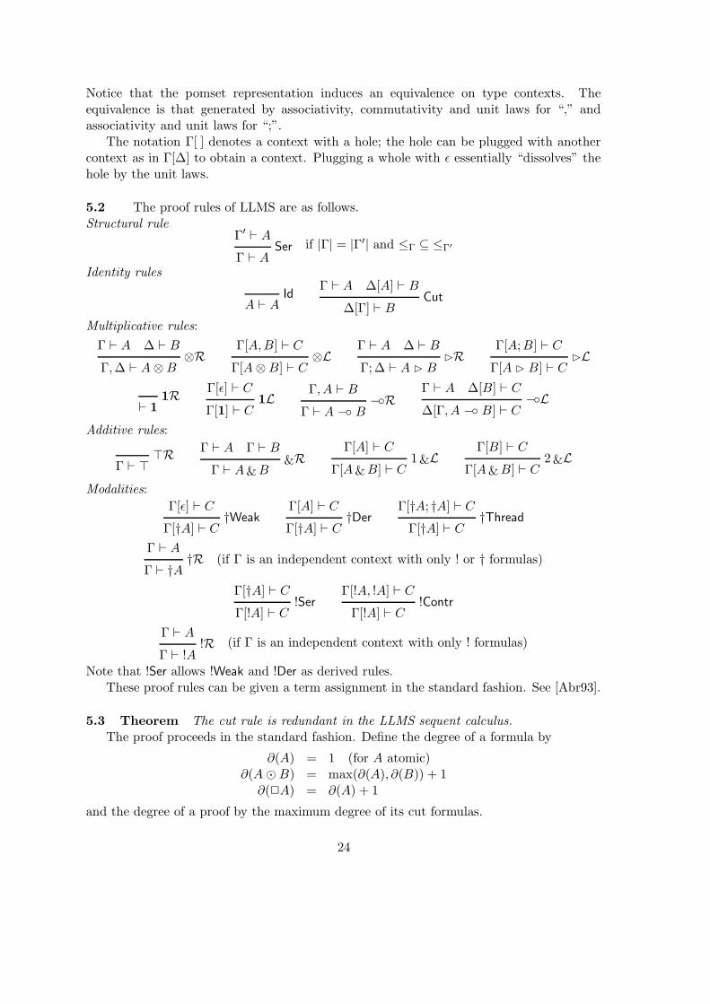
Notice that the pomset representation induces an equivalence on type contexts. Theequivalence is that generated by associativity, commutativity and unit laws for “,” andassociativity and unit laws for “;”.

The notation Γ[ ] denotes a context with a hole; the hole can be plugged with anothercontext as in Γ[∆] to obtain a context. Plugging a whole with ε essentially “dissolves” thehole by the unit laws.

5.2 The proof rules of LLMS are as follows.Structural rule

Γ′ ` ASer

Γ ` Aif |Γ| = |Γ′| and ≤Γ ⊆ ≤Γ′

Identity rules

IdA ` A

Γ ` A ∆[A] ` BCut

∆[Γ] ` B

Multiplicative rules:

Γ ` A ∆ ` B⊗R

Γ,∆ ` A⊗B

Γ[A,B] ` C⊗L

Γ[A⊗B] ` C

Γ ` A ∆ ` BBR

Γ;∆ ` A B B

Γ[A;B] ` CBL

Γ[A B B] ` C

1R` 1

Γ[ε] ` C1L

Γ[1] ` C

Γ, A ` B−◦R

Γ ` A −◦ B

Γ ` A ∆[B] ` C−◦L

∆[Γ, A −◦ B] ` C

Additive rules:

>RΓ ` >

Γ ` A Γ ` B&R

Γ ` A&B

Γ[A] ` C1&L

Γ[A&B] ` C

Γ[B] ` C2&L

Γ[A&B] ` C

Modalities:

Γ[ε] ` C†Weak

Γ[†A] ` C

Γ[A] ` C†Der

Γ[†A] ` C

Γ[†A; †A] ` C†Thread

Γ[†A] ` C

Γ ` A†R

Γ ` †A(if Γ is an independent context with only ! or † formulas)

Γ[†A] ` C!Ser

Γ[!A] ` C

Γ[!A, !A] ` C!Contr

Γ[!A] ` C

Γ ` A!R

Γ ` !A(if Γ is an independent context with only ! formulas)

Note that !Ser allows !Weak and !Der as derived rules.These proof rules can be given a term assignment in the standard fashion. See [Abr93].

5.3 Theorem The cut rule is redundant in the LLMS sequent calculus.

The proof proceeds in the standard fashion. Define the degree of a formula by

∂(A) = 1 (for A atomic)∂(A�B) = max(∂(A), ∂(B)) + 1∂(2A) = ∂(A) + 1

and the degree of a proof by the maximum degree of its cut formulas.

24

5.4 Lemma If A is a formula of degree d and Γ ` A and ∆[A] ` B have proofs π and

π′ of degree smaller than d then ∆[Γ] ` B has a proof of degree smaller than d.The proof is by induction on the sum of the heights of the two given proofs. If π and π ′

end in Id or right and left rules for A (the structural rules of the modalities are consideredleft rules), then the symmetries of the rules allow reduction in the height of one proof. Forexample,

Γ ` A!R

Γ ` !A

∆[†A] ` B!Ser

∆[!A] ` BCut

∆[Γ] ` B

=⇒

Γ ` A†R

Γ ` †A ∆[†A] ` BCut

∆[Γ] ` B

By inductive hypothesis, we conclude that ∆[Γ] ` B has a proof of degree smaller than d.If π and π′ end in left/right rules for some other formula, then we consider some

appropriate subproofs of π and π′ for inductive hypothesis. 2

It can then be shown that every proof of degree d > 0 is reducible to a proof of a smallerdegree. Hence, the theorem follows.

5.5 Theorem The LLMS proof system has a semantics in COHL, in fact, in any

LLMS-category. Further, this semantics is preserved by cut elimination.

The interpretation of a context is as mentioned in 5.1. A sequent Γ ` A is interpretedas a linear map Γ −◦ A.

The interpretation of most rules follow from the properties of COHL (and other LLMS-categories) mentioned in Sec. 2. The only rules that need some care are †R and !R. Consider†R. Since Γ is an independent context, it is of the form !C1, . . . , !Cn, †D1, . . . , †Dm. Thefact that ! and † are monoidal comonads (cf. 2.18) gives the following map:

Γ = (⊗

!Ci) ⊗ (⊗

†Dj)(⊗

Dup)⊗(⊗

Seq)- (

⊗!!Ci) ⊗ (

⊗††Dj)

(⊗

Ser)⊗id- (

⊗†!Ci) ⊗ (

⊗††Dj)

sprom- †((

⊗!Ci) ⊗ (

⊗†Dj)) = †Γ

†[[Γ`A]]- †A

The interpretation of !R is similar.It is a routine exercise to check that cut-elimination preserves the semantics.

5.6 Since the correspondence between LLMS-categories and the LLMS proof system israther close, the interpretation of Algol given in Sec. 4 can be easily adapted to a translationto LLMS. This shows that LLMS is a rich framework for modelling state-manipulations.

One might wonder if we can use LLMS (with an appropriate term assignment) as aprogramming language. At this stage, such an exercise would seem unwise. The type systemrepresented by LLMS is quite complex, with two kinds of connectives in type contexts. Incontrast, interference-controlled Algol seems to hide much of this complexity by using agood set of combinators. While it is an open question whether LLMS can give rise to aprogramming framework that is superior to Algol, we believe the best use of LLMS is as

25

a conceptual model for thinking about programs in Algol and other languages supportingstate-manipulation.

6 Conclusion

We have described here a logical model for state-manipulation using the framework oflinear logic. The model is characterized abstractly in terms of a proof system as well as acategorical definition and, also, concretely in terms of coherent spaces. It is demonstratedthat the model is able to handle nontrivial programming languages incorporating state-manipulation.

Many issues need further resolution. The most immediate one is modelling passivity.There seem to be two possibilities. One is to enrich coherent spaces with an “independencerelation” to obtain, say, “independence spaces” and then treat †A as the free partiallyco-commutative comonoid generated by the independence space A. See [CF69, Per86] forthe algebraic concepts, which have been used for modelling Petri nets [Maz89]. !A is thena special case of †A when A is fully independent (so that †A becomes co-commutative). Infact, independence spaces have two choices for “with”: an independent product & and adependent product &D. The former has the rather surprising property: †(A&B) ∼= †A⊗†B.Another possibility is to use “correlation spaces” as in [Gir91]. An active correlation spaceis what we get by † in the world of coherent spaces. So, active correlation spaces arecomonoids. Passive correlation spaces (the same as Girard’s positive correlation spaces)can then be treated as the special case of co-commutative comonoids.

Game semantics is another exciting avenue. Note that “before” has quite simple inter-pretation in Abramsky-Jagadeesan games [AJ92, AJM93]. A B B is the game that allowsone-way switching for both the Player and the Opponent. This can in fact be extendedto an LLMS-category of games which, not surprisingly, involve history-sensitive strategies.The issue here, again, is modelling passivity.

Much work remains to be done in developing a “theory” of state-manipulation using thismodel. The additional equivalences, which are not presently captured, must be studied. Thetrace-based model also need to be related to the traditional state-based models. Finally,reasoning principles must be developed as in, for example, [Hoa85, MT92].

Acknowledgements I owe much debt to Peter O’Hearn for numerous discussions andencouragement. His work on relating linear logic and interference control was the startingpoint for this work. Thanks are also due to Samson Abramsky, Radha Jagadeesan, BobTennent and Sam Kamin for contributing to this work in various ways through theirdiscussions.

A A brief review of classical features

... to be filled in.Essentially, define A⊥ ∼= A −◦ 1 and A

...............................................................................................B = A⊥ −◦ B.

26

References

[Abr93] S. Abramsky. Computational interpretations of linear logic. Theoretical Comp.

Science, 111(1-2):3–57, 1993.[AJ92] S. Abramsky and R. Jagadeesan. Games and full completeness for multiplicative

linear logic. Manuscript, Imperial College, 1992. (available by ftp fromtheory.doc.ic.ac.uk, directory /theory/papers/Abramsky.).

[AJM93] S. Abramsky, R. Jagadeesan, and P. Malacaria. Games and full ab-straction for PCF: Preliminary announcement. Manuscript, Imperial Col-lege, July 1993. (available by ftp from theory.doc.ic.ac.uk, directory /the-ory/papers/Abramsky.).

[Ber78] G. Berry. Stable models of typed λ-calculi. In Fifth Intern. Colloq. Automata,

Languages. and Programming, volume 62 of Lect. Notes in Comp. Science, pages72–88. Springer-Verlag, 1978.

[Bri73] P. Brinch Hansen. Operating Systems Principles. Prentice Hall, 1973.[CF69] P. Cartier and D. Foata. Problemes Combinatoires de Commutation et

Rearrangements, volume 85 of Lect. Notes in Math. Springer-Verlag, 1969.[Gir87a] J.-Y. Girard. Linear logic. Theoretical Comp. Science, 50:1–102, 1987.[Gir87b] J.-Y. Girard. Towards a geometry of interaction. In J. W. Gray and

A. Scedrov, editors, Categories in Computer Science and Logic, pages 69–108,Boulder, Colorado, June 1987. American Mathematical Society. (ContemporaryMathematics, Vol. 92).

[Gir91] J.-Y. Girard. A new constructive logic: Classical logic. Prepublication 24,Equipe de Logique, University of Paris VII, May 1991.

[GL86] D.K. Gifford and J.M. Lucassen. Integrating functional and imperativeprogramming. In ACM Symp. on LISP and Functional Programming, pages28–38, 1986.

[GLT89] J-Y. Girard, Y. Lafont, and P. Taylor. Proofs and Types. Cambridge Univ.Press, Cambridge, 1989.

[Gun92] C. A. Gunter. Semantics of Programming Languages: Structures and Tech-

niques. MIT Press, 1992.[HMRC87] R. C. Holt, P. A. Matthews, J. A. Rosselet, and J. R. Cordy. The Turing

Programming Language. Prentice Hall, 1987.[Hoa85] C. A. R. Hoare. Communicating Sequential Processes. Prentice-Hall Interna-

tional, London, 1985.[Jac92] B. Jacobs. Semantics of weakening and contraction. Manuscript, Cambridge

University, Nov 1992.[Koc72] A. Kock. Strong functors and monoidal monads. Archiv. der Mathematik,

XXIII:113–120, 1972.[Laf88] Y. Lafont. The linear abstract machine. Theoretical Comp. Science, 59:157–180,

1988.[Mac71] S. MacLane. Categories for the Working Mathematician. Springer-Verlag, 1971.[Maz89] A. Mazurkiewicz. Basic notions of trace theory. In J. S. de Bakker, W.-P.

de Roever, and G. Rozenberg, editors, Linear Time, Branching Time and

Partial Order in Logics and Models of Concurrency, volume 354 of Lect. Notes

27

in Comp. Science, pages 285–363. Springer-Verlag, 1989.[Mil89] R. Milner. Communication and Concurrency. Prentice Hall, 1989.[MS88] A. R. Meyer and K. Sieber. Towards fully abstract semantics for local variables.

In Fifteenth Ann. ACM Symp. on Princ. of Program. Lang., pages 191–203.ACM, 1988.

[MT92] I. A. Mason and C. L. Talcott. References, local variables and operationalreasoning. In Proceedings, Seventh Annual IEEE Symposium on Logic in

Computer Science, pages 186–197, Santa Cruz, California, 22–25 June 1992.IEEE Computer Society Press.

[Nau60] P. Naur, et. al. Report on the algorithmic language ALGOL 60. Comm. ACM,3(5):299–314, May 1960.

[O’H] P. W. O’Hearn. A model for syntactic control of interference. Math. Structures

in Comp. Science. (to appear).[O’H91] P. W. O’Hearn. Linear logic and interference control. In D. H. Pitt, editor,

Category Theory and Computer Science, volume 350 of Lect. Notes in Comp.

Science, pages 74–93. Springer-Verlag, 1991.[Ole85] F. J. Oles. Type algebras, functor categories and block structure. In M. Nivat

and J. C. Reynolds, editors, Algebraic Methods in Semantics, pages 543–573.Cambridge Univ. Press, Cambridge, U. K., 1985.

[ORH93] M. Odersky, D. Rabin, and P. Hudak. Call by name, assignment and the lambdacalculus. In Twentieth Ann. ACM Symp. on Princ. of Program. Lang. ACM,1993.

[OT93] P. W. O’Hearn and R. D. Tennent. Relational parametricity and local variables.In Twentieth Ann. ACM Symp. on Princ. of Program. Lang., pages 171–184.ACM, 1993.

[Per86] D. Perrin. Words over a partially commutative alphabet. In A. Apostolico andZ. Galil, editors, Combinatorial Algorithms on Words, volume 12 of NATO ASI

Series, pages 329–340. Springer-Verlag, 1986.[PM87] D. Pountain and D. May. A Tutorial Introduction to Occam Programming.

McGraw-Hill, 1987.[Pop77] G. J. Popek et. al. Notes on the design of EUCLID. SIGPLAN Notices, 12(3):11–

18, 1977.[PW93] S. L. Peyton Jones and P. Wadler. Imperative functional programming. In

Twentieth Ann. ACM Symp. on Princ. of Program. Lang. ACM, 1993.[Red93] U. S. Reddy. A linear logic model of state (extended abstract). Technical report,

University of Glasgow, Jan 1993. (also available by ftp from theory.doc.ic.ac.uk,directory /theory/papers/Reddy.).

[Ret93a] C. Retore. Pomset logic: A truly concurrent linear calculus. Draft, Ecole desMines de Paris, Sophia Antipolis, France, 1993.

[Ret93b] C. Retore. Reseaux et Sequents Ordonnes Mathematiques. PhD thesis,Universite Paris 7, Fevrier 1993.

[Rey78] J. C. Reynolds. Syntactic control of interference. In ACM Symp. on Princ. of

Program. Lang., pages 39–46. ACM, 1978.[Rey81] J. C. Reynolds. The essence of Algol. In J. W. de Bakker and J. C. van Vliet,

editors, Algorithmic Languages, pages 345–372. North-Holland, 1981.

28

[Rey89] J. C. Reynolds. Syntactic control of interference, Part II. In Intern. Colloq.

Automata, Languages. and Programming, volume 372 of Lect. Notes in Comp.

Science, pages 704–722. Springer-Verlag, 1989.[See89] R. A. G. Seely. Linear logic, *-autonomous categories and cofree coalgebras.

In J. W. Gray and A. Scedrov, editors, Categories in Computer Science and

Logic, volume 92 of Contemporary Mathematics, pages 371–382. AmericanMathematical Society, 1989.

[SRI91] V. Swarup, U. S. Reddy, and E. Ireland. Assignments for applicative languages.In R. J. M. Hughes, editor, Conf. on Functional Program. Lang. and Comput.

Arch., volume 523 of Lect. Notes in Comp. Science, pages 192–214. Springer-Verlag, 1991.

[Sto77] J. E. Stoy. Denotational Semantics: The Scott–Strachey Approach to Program-

ming Language Theory. MIT Press, 1977.[Wad90] P. Wadler. Linear types can change the world! In M. Broy and C. B. Jones,

editors, Programming Concepts and Methods. North-Holland, Amsterdam, 1990.(Proc. IFIP TC 2 Working Conf., Sea of Galilee, Israel).

[Wad91] P. Wadler. Is there a use for linear logic? In Proc. Symp. on Partial

Evaluation and Semantics-Based Program Manipulation, pages 255–273. ACM,1991. (SIGPLAN Notices, Sep. 1991).

[Win80] G. Winskel. Events in Computation. PhD thesis, Univ. of Edinburgh, 1980.[Win87] G. Winskel. Event structures. In W. Brauer, W. Reisig, and G. Rozen-

berg, editors, Petri Nets: Applications and Relationships to Other Models of

Concurrency, volume 255 of Lect. Notes in Comp. Science, pages 325–392.Springer-Verlag, 1987.

[Zha92] G.-Q. Zhang. DI-domains as prime information systems. Information and

Computation, 100(2):151–177, 1992.[Zha93] G.-Q. Zhang. Some monoidal closed categories of stable domains and event

structures. Math. Structures in Comp. Science, 3:259–276, 1993.

29