a lender-based theory of collateral - uni- · pdf filea lender-based theory of collateral$ ......
TRANSCRIPT

ARTICLE IN PRESS
Journal of Financial Economics 84 (2007) 826–859
0304-405X/$
doi:10.1016/j
$We than
participants a
the Federal R
Meetings in P
Liquidity Co
financial supp�Correspo
Tel.: +1 212
E-mail ad
www.elsevier.com/locate/jfec
A lender-based theory of collateral$
Roman Indersta,c, Holger M. Muellerb,c,�
aLondon School of Economics, Houghton Street, London WC2A 2AE, UKbStern School of Business, New York University, New York, NY 10012, USA
cCentre for Economic Policy Research (CEPR), London EC1V 7RR, UK
Received 7 April 2004; received in revised form 4 May 2006; accepted 13 June 2006
Available online 4 March 2007
Abstract
We consider an imperfectly competitive loan market in which a local relationship lender has an
information advantage vis-a-vis distant transaction lenders. Competitive pressure from the
transaction lenders prevents the local lender from extracting the full surplus from projects. As a
result, the local lender inefficiently rejects marginally profitable projects. Collateral mitigates the
inefficiency by increasing the local lender’s payoff from precisely those marginally profitable projects
that she inefficiently rejects. The model predicts that, controlling for observable borrower risk,
collateralized loans are more likely to default ex post, which is consistent with the empirical evidence.
The model also predicts that borrowers for whom local lenders have a relatively smaller information
advantage face higher collateral requirements, and that technological innovations that narrow the
information advantage of local lenders, such as small business credit scoring, lead to a greater use of
collateral in lending relationships.
r 2007 Elsevier B.V. All rights reserved.
JEL classification: D82; G21
Keywords: Collateral; Soft information; Loan market competition; Relationship lending
- see front matter r 2007 Elsevier B.V. All rights reserved.
.jfineco.2006.06.002
k an anonymous referee, Patrick Bolton, Anthony Lynch, Ernst Maug, Jeff Wurgler, and seminar
t Princeton University, New York University, London School of Economics, Cambridge University,
eserve Bank of Philadelphia, University of Frankfurt, the American Finance Association (AFA)
hiladelphia, the Financial Intermediation Research Society (FIRS) Conference in Capri, and the
nference at the London School of Economics for helpful comments. Roman Inderst acknowledges
ort from the Financial Markets Group (FMG).
nding author. Stern School of Business, New York University, New York, NY 10012, USA.
998 0341.
dress: [email protected] (H.M. Mueller).

ARTICLE IN PRESSR. Inderst, H.M. Mueller / Journal of Financial Economics 84 (2007) 826–859 827
1. Introduction
About 80% of small business loans in the United States are secured by collateral (Avery,Bostic, and Samolyk 1998). Understanding the role of collateral is important, not onlybecause of its widespread use, but also because of its implications for monetary policy. Forexample, under the financial accelerator view of monetary policy transmission, a tighteningof monetary policy and the associated increase in interest rates impairs collateral values,making it more difficult for borrowers to obtain funds, which reduces investment andeconomic growth (see, e.g., Bernanke, Gertler, and Gilchrist 1999).
Over the past decade, small business lending in the United States has witnessed aninformation revolution (Petersen and Rajan, 2002). Small business lending has historicallybeen a local activity based on soft information culled from close contacts with borrowersand knowledge of local conditions. This picture has changed. Advances in informationtechnology, in particular the widespread adoption of small business credit scoring, havemade it possible to underwrite transaction loans based solely on publicly available hardinformation without meeting the borrower.1 As a result, local lenders have faced increasingcompetitive pressure from arm’s-length transaction lenders, especially large banks(Hannan, 2003; Frame, Padhi, and Woosley, 2004; Berger, Frame, and Miller, 2005).
These developments raise important questions. As the competitive pressure fromtransaction lenders increases, what will happen to collateral requirements? Will locallenders reduce their collateral requirements, implying that collateral might lose itsimportance for small business lending? Or will collateral requirements increase? And whowill be affected the most by the changes in collateral requirements: businesses for whichlocal lenders have a strong information advantage vis-a-vis transaction lenders, orbusinesses for which the information advantage of local lenders is weak?
This paper proposes a novel theory of collateral that can address these questions. Ourmodel has no borrower moral hazard or adverse selection. We consider an imperfectlycompetitive loan market in which a local lender has an information advantage vis-a-visdistant transaction lenders. The local lender has privileged access to soft privateinformation that enables her to make a more precise estimate of the borrower’s defaultlikelihood. This provides the local lender with a competitive advantage, which generallyallows her to attract local borrowers.2 Nevertheless, competition from transaction lendersprovides borrowers with a positive outside option that the local lender must match. Toattract a borrower, the local lender must offer him a share of the project’s cash flow, whichdistorts the local lender’s credit decision. As the local lender incurs the full project cost but
1Two pieces of hard information are especially important: the business owner’s personal credit history, obtained
from consumer credit bureaus, and information on the business itself, obtained from mercantile credit
information exchanges, such as Dun and Bradstreet. While credit scoring has been used for some time in
consumer lending, it has only recently been applied to small business lending after it was found that the business
owner’s personal credit history is highly predictive of the loan repayment prospects of the business. For an
overview of small business credit scoring, see Mester (1997) and Berger and Frame (2007).2This is consistent with the observation by Petersen and Rajan (1994, 2002) that 95% of the smallest firms in
their sample borrow from a single lender (1994), which is generally a local bank (2002). See also Petersen and
Rajan (1995), who argue that credit markets for small firms are local, and Guiso et al. (2004), who refer to direct
evidence of the information disadvantage of distant lenders in Italy. As in our model, Hauswald and Marquez
(2003, 2006) and Almazan (2002) assume that lenders who are located closer to a borrower have better
information about the borrower. Our notion of imperfect loan market competition differs from Thakor (1996),
who considers symmetric competition between multiple lenders.

ARTICLE IN PRESSR. Inderst, H.M. Mueller / Journal of Financial Economics 84 (2007) 826–859828
receives only a fraction of the cash flow, she accepts only projects whose expected cash flowis sufficiently greater than the cost. That is, the local lender rejects projects with a small butpositive net present value (NPV).Collateral can mitigate the inefficiency.3 The fundamental role of collateral in our model
is to flatten the local lender’s payoff function. When collateral is added, the local lender’spayoff exceeds the project cash flow in low cash flow states. The local lender’s payoff inhigh cash flow states must be reduced, or else the borrower’s participation constraint isviolated. However, as low cash flows are more likely under low-NPV projects, the overalleffect is that the local lender’s payoff from low-NPV projects—and therefore fromprecisely those projects that she inefficiently rejects—increases. Hence, collateral improvesthe local lender’s incentives to accept marginally positive projects, making her creditdecision more efficient.We consider two implications of the information revolution in small business lending,
both of which lead to greater competitive pressure from transaction lenders. The firstimplication is that the credit scoring information advantage of local lenders vis-a-vistransaction lenders has narrowed. Small business credit scoring models can predict thelikelihood that a loan applicant will default fairly accurately, thus reducing the informationuncertainty associated with small business loans made to borrowers located far away(Mester, 1997). In our model, a narrowing of the local lender’s information advantage vis-a-vis transaction lenders forces the local lender to reduce the loan rate, implying that theborrower receives a larger share of the project’s cash flow. To minimize distortions in hercredit decision, the local lender must raise the collateral requirement. Our model thuspredicts that, following the widespread adoption of small business credit scoring the use ofcollateral in lending relationships should increase. We also obtain a cross-sectionalprediction, namely, that borrowers for whom the local lender has a relatively smallerinformation advantage should face higher collateral requirements. Consistent with thisprediction, Petersen and Rajan (2002) find that small business borrowers who are locatedfarther away from their local lender are more likely to pledge collateral.The second implication of the information revolution in small business lending that we
consider is that the direct costs of underwriting transaction loans have decreased. Similarto above, this increases the competitive pressure from transaction lenders, implying thatthe local lender must reduce the loan rate and raise the collateral requirement. Our modelthus predicts that technological innovations that reduce the costs of underwritingtransaction loans should lead to a greater use of collateral in local lending relationships.Moreover, the increase in collateral should be weaker for borrowers for whom the locallender has a relatively greater information advantage.As the sole role of collateral in our model is to minimize distortions in credit decisions
based on soft private information, collateral has no meaningful role to play in loansunderwritten by transaction lenders. While the vast majority of small business loans in theUnited States are collateralized, small business loans made by transaction lenders on thebasis of credit scoring tend to be unsecured (Zuckerman, 1996; Frame, Srinivasan, andWoosley, 2001; Frame, Padhi, and Woosley, 2004).
3That the local lender’s credit decision is based on soft private information is crucial for the inefficiency and,
hence, also for our argument for collateral. If the information were contractible, the local lender could commit to
the first-best credit decision, even if it meant committing to a decision rule that is ex post suboptimal. Likewise, if
the information were observable but nonverifiable, the inefficiency could be eliminated through bargaining.

ARTICLE IN PRESSR. Inderst, H.M. Mueller / Journal of Financial Economics 84 (2007) 826–859 829
We are not aware of empirical studies that examine how an increase in competitivepressure from arm’s-length transaction lenders affects the use of collateral in local lendingrelationships. However, Jimenez and Saurina (2004) and Jimenez, Salas, and Saurina(2006a) provide some indirect support for our model. Using Spanish data, they find apositive relation between collateral and bank competition, as measured by the Herfindahlindex. Moreover, Jimenez, Salas, and Saurina (2006b) find that this positive effect isweaker if the duration of borrower relationships is shorter, which is consistent with ourmodel if the information advantage of local lenders increases with the duration ofborrower relationships.
To the best of our knowledge, related models of imperfect loan market competition,such as Boot and Thakor (2000), who consider competition between transaction lendersand relationship lenders, or Hauswald and Marquez (2003, 2006), who examine howinformation technology affects competition between differentially informed lenders, do notconsider collateral. Likewise, Inderst and Mueller (2006), who analyze the optimal securitydesign in a model similar to this paper, do not consider collateral. On the other hand, tothe extent that they consider loan market competition, models of collateral do not considerimperfect competition between arm’s-length transaction lenders and local relationshiplenders, thus making empirical predictions that are different from ours. For example,Besanko and Thakor (1987a) and Manove, Padilla, and Pagano (2001) both compare amonopolistic with a perfectly competitive loan market and find that collateral is used onlyin the latter. Closer in spirit to our model, Villas-Boas and Schmidt-Mohr (1999) consideran oligopolistic loan market with horizontally differentiated banks, showing that collateralrequirements can either increase or decrease as bank competition increases.4
In addition to examining the role of imperfect loan market competition for collateral,our model also makes predictions for a given borrower–lender relationship, that is, holdingloan market competition constant. For instance, our model predicts that observably riskierborrowers should pledge more collateral and that, holding observable borrower riskconstant, collateralized loans are more likely to default ex post. Both predictions areconsistent with the empirical evidence. Observably riskier borrowers indeed appear topledge more collateral (Leeth and Scott, 1989; Berger and Udell, 1995; Dennis, Nandy, andSharpe, 2000), and, controlling for observable borrower risk, collateralized loans indeedappear to be riskier in the sense that they default more often (Jimenez and Saurina, 2004;Jimenez, Salas, and Saurina, 2006a) and have worse performance in terms of paymentspast due and nonaccruals (Berger and Udell, 1990).
The above two predictions do not easily follow from existing models of collateral.Adverse selection models (Bester, 1985; Chan and Kanatas, 1985; Besanko and Thakor,1987a,b) predict that safer borrowers within an observationally identical risk pool pledgemore collateral. Likewise, moral-hazard models (Chan and Thakor, 1987; Boot andThakor, 1994) are based on the premise that posting collateral improves borrowers’incentives to work hard, reducing their likelihood of default. An exception is Boot,Thakor, and Udell (1991), who combine observable borrower quality with moral hazard.Like this paper, they also find that observably riskier borrowers may pledge more
4Villas-Boas and Schmidt-Mohr (1999) consider a spatial competition model with two banks located at the
endpoints of a line. Entrepreneurs incur travel costs that depend on the distance they must travel to each bank.
Unlike this paper, entrepreneurs are better informed than banks, while the two banks have the same information
about entrepreneurs.
ARTICLE IN PRESSR. Inderst, H.M. Mueller / Journal of Financial Economics 84 (2007) 826–859830
collateral and that collateralized loans may be riskier ex post. Intuitively, if borrowerquality and effort are substitutes, low-quality borrowers post collateral to commit tohigher effort. While this reduces the default likelihood of low-quality borrowers, thelikelihood remains still higher than it is for high-quality borrowers because of the greaterrelative importance of borrower quality for default risk.5
Most existing models of collateral assume agency problems on the part of the borrower.Notable exceptions are Rajan and Winton (1995) and Manove, Padilla, and Pagano (2001).Rajan and Winton (1995) examine the effect of collateral on the lender’s ex post monitoringincentives. Monitoring is valuable in their model because it allows the lender to claimadditional collateral if the firm is in distress. In Manove, Padilla, and Pagano (2001),lenders that are protected by collateral screen too little. In our model, by contrast, collateraland screening are complements. Without screening, there would be no role for collateral.The rest of this paper is organized as follows. Section 2 lays out the basic model.
Section 3 focuses on a given borrower–lender relationship. It shows why collateral isoptimal in our model, derives comparative static results, and discusses related empiricalliterature. Section 4 considers robustness issues. Section 5 examines how technologicalinnovations that increase the competitive pressure from transaction lenders affect the use ofcollateral in local lending relationships. The related empirical literature is discussed alongwith our empirical predictions. Section 6 concludes. Appendix A shows that our basicargument for collateral extends to a continuum of cash flows. All proofs are in Appendix B.
2. The model
In this section, we present a simple model in which a local relationship lender makes heraccept or reject decision based on soft private information about the borrower.
2.1. Basic setup
A firm (the borrower) has an indivisible project with fixed investment cost k40.6 Theproject cash flow x is verifiable and can be either high ðx ¼ xhÞ or low ðx ¼ xlÞ. The twocash flow model is the simplest framework to illustrate our novel argument for collateral.Appendix A shows that our argument straightforwardly extends to a setting with acontinuum of cash flows. The borrower has pledgeable assets w, where xl þ wok, implyingthat the project cannot be financed by issuing a safe claim. The risk-free interest rate isnormalized to zero.
2.2. Lender types and information structure
There are two types of lenders: a local lender and distant transaction lenders.Transaction lenders are perfectly competitive and provide arm’s-length financing based
5There are fundamental differences between Boot, Thakor, and Udell (1991) and this paper. First, the role of
collateral in Boot, Thakor, and Udell’s model is to mitigate agency problems on the part of the borrower. In our
model, the role of collateral is to mitigate incentive problems on the part of the lender. Second, Boot, Thakor, and
Udell consider a perfectly competitive loan market in which lenders earn zero expected profits, while we consider
an imperfectly competitive loan market in which better informed local lenders earn positive expected profits.6With few exceptions (for example, Besanko and Thakor, 1987b), existing models of collateral assume a fixed
project size.

ARTICLE IN PRESSR. Inderst, H.M. Mueller / Journal of Financial Economics 84 (2007) 826–859 831
solely on publicly available hard information.7 Given this information, the project’ssuccess probability is Prðx ¼ xhÞ :¼ p 2 ð0; 1Þ. The corresponding expected cash flow ism :¼ pxh þ ð1� pÞxl .
The difference between the local lender and transaction lenders is that the local lender hasprivileged access to soft information, allowing her to make a more precise estimate of theproject’s success probability. For example, the local lender could already be familiar withthe borrower from previous lending relationships. But even if the local lender has no priorlending relationship with the borrower, managing the borrower’s accounts, familiarity withlocal conditions, and experience with similar businesses in the region may provide the locallender with valuable information that the transaction lenders do not have.8
We assume that the local lender’s assessment of the borrower’s project can be representedby a continuous variable s 2 ½0; 1� with associated success probability ps. In practice, s and ps
could be viewed as the local lender’s internal rating of the borrower. The success probabilityps is increasing in s, implying that the conditional expected project cash flow ms :¼ psxh þ
ð1� psÞxl is also increasing in s. Because the local lender’s assessment is based on softinformation that is difficult to verify vis-a-vis outsiders, we assume that s and ps are privateinformation.9 As for the borrower, we assume that he lacks the skill and expertise to replicatethe local lender’s project evaluation. After all, professional lenders have specialized expertise,which is why they are in the project-evaluation business.10 In sum, neither the transactionlenders (for lack of access to soft information) nor the borrower (for lack of expertise) canobserve s or ps. Of course, the expected value of ps is commonly known: consistency of beliefsrequires that p ¼
R 10 psf ðsÞds, where f ðsÞ is the density associated with s.
To make the local lender’s access to soft information valuable, we assume that m14k
and m0ok. That is, the project’s NPV is positive for high s and negative for low s.Consequently, having access to soft information allows the local lender to distinguishbetween positive- and negative-NPV projects. By contrast, transaction lenders can onlyobserve the project’s NPV based on publicly available hard information, which is m� k.
2.3. Financial contracts
A financial contract specifies repayments tlpxl and thpxh out of the project’s cash flow,an amount of collateral Cpw to be pledged by the borrower, and repayments clpC and
7The term ‘‘transaction lending’’ is from Boot and Thakor (2000). In their model, as in ours, transaction lenders
create no additional value other than providing arm’s-length financing.8As Mester (1997, p. 12) writes, ‘‘[T]he local presence gives the banker a good knowledge of the area, which is
thought to be useful in the credit decision. Small businesses are likely to have deposit accounts at the small bank in
town, and the information the bank can gain by observing the firm’s cash flows can give the bank an information
advantage in lending to these businesses.’’9As Brunner, Krahnen, and Weber (2000, p. 4) argue, ‘‘[I]nternal ratings should therefore be seen as private
information. Typically, banks do not inform their customers of the internal ratings or the implied PODs
[probabilities of default], nor do they publicize the criteria and methods used in deriving them.’’ See also Manove,
Padilla, and Pagano (2001), who note that ‘‘the information [collected by relationship lenders] remains
confidential (proprietary).’’10See Manove, Padilla, and Pagano (2001). If the local lender also holds loans from other local businesses, she
may know more than any individual borrower, because she knows where the borrower’s local competitors are
headed (Boot and Thakor, 2000). Consistent with the notion that professional lenders are better than borrowers at
estimating default risk, Reid (1991) finds that bank-financed firms are more likely to survive than firms funded by
family investors.

ARTICLE IN PRESSR. Inderst, H.M. Mueller / Journal of Financial Economics 84 (2007) 826–859832
chpC out of the pledged assets. The total repayment made by the borrower is thusRl :¼ tl þ cl in the bad state and Rh :¼ th þ ch in the good state.11
Given that the local lender has interim private information, a standard solution isto have the local lender offer an incentive-compatible menu of contracts from whichshe chooses after evaluating the borrower’s project. Introducing such a menu is sub-optimal in our model (see Section 4.2). Instead, it is uniquely optimal to havethe local lender offer a single contract, and then have her accept or reject the borroweron the basis of this contract. This is consistent with the notion that, in manyloan markets, credit decisions are plain accept-or-reject decisions: loan applicants areeither accepted under the terms of the initial contract offer or rejected (Saunders andThomas, 2001).
2.4. Timeline and competitive structure of the loan market
There are three dates: t ¼ 0, t ¼ 1, and t ¼ 2. In t ¼ 0, the local lender and transactionlenders make competing offers. As transaction lenders have only access to publicinformation, making an offer to the borrower is de facto equivalent to accepting him. If theborrower goes to the local lender, the local lender evaluates the borrower’s project, whichtakes place in t ¼ 1. If the borrower is accepted, he obtains financing under the terms ofthe initial offer.12 If the borrower is rejected, he can still seek financing from transactionlenders. In t ¼ 2, the project’s cash flow is realized, and the borrower makes thecontractually stipulated repayment.To ensure the existence of a pure-strategy equilibrium, we assume that transaction
lenders can observe whether the borrower has sought credit from the local lender.13
Given that the transaction lenders are perfectly competitive, they can thus offer a borrowerwho has not previously sought credit from the local lender the full project NPV based onhard information. In contrast, we assume that the local lender makes a take-it-or-leave-itoffer that maximizes her own profits, subject to matching the borrower’s outside optionfrom going to transaction lenders. Effectively, we thus give the local lender all of thebargaining power. Section 4.1 shows that our results extend to arbitrary distributions ofbargaining powers. This also includes the other polar case in which the contract offermaximizes the borrower’s expected profits. Moreover, Section 4.2 shows that the locallender and the borrower will not renegotiate the initial contract after the projectevaluation.
11This excludes the possibility that the local lender ‘‘buys’’ the project before evaluating it. Using a standard
argument, we assume that up-front payments from the local lender would attract a potentially large pool of
fraudulent borrowers, or ‘‘fly-by-night operators,’’ who have fake projects (see Rajan, 1992). This argument also
rules out that the local lender pays a penalty to the borrower if the loan is not approved.12Section 4.2 revisits our assumption that the local lender makes an offer before the project evaluation. At least
in the case of small business lending, lenders appear to make conditional ex ante offers specifying what loan terms
borrowers will receive if the loan application is approved. At Chase Manhattan, for instance, applicants for small
business loans are shown a pricing chart explaining in detail what interest rate they will get if their loan is
approved. A copy of the pricing chart is available from the authors.13On the nonexistence of pure-strategy equilibria in loan markets with differentially informed lenders, see
Broecker (1990). When a borrower applies for a loan, the lender typically inquires into the borrower’s credit
history, which is subsequently documented in the borrower’s credit report. Hence, future lenders can see if, when,
and from whom the borrower has previously sought credit (Mester, 1997; Jappelli and Pagano, 2002).

ARTICLE IN PRESSR. Inderst, H.M. Mueller / Journal of Financial Economics 84 (2007) 826–859 833
3. Optimal credit decision and financial contract
In our analysis of loan market competition in Section 5, we will show that the locallender may be sometimes unable to attract the borrower. Formally, there may be nosolution to the local lender’s maximization problem that satisfies the borrower’sparticipation constraint. In this section, we solve the local lender’s maximization problemassuming that a solution exists. We first characterize general properties of the local lender’soptimal credit decision (Section 3.1) and financial contract (Section 3.2). We then examinehow the optimal contract depends on the borrower’s pledgeable assets (Section 3.3).We conclude with a comparative static analysis and discussion of the empirical literature(Section 3.4).
3.1. General properties of the optimal credit decision
We begin with the first-best optimal credit decision. Given that msok for low s andms4k for high s, and given that ms is increasing and continuous in s, there exists a uniquefirst-best cutoff sFB 2 ð0; 1Þ given by msFB
¼ k such that the project’s NPV is positive ifs4sFB, zero if s ¼ sFB, and negative if sosFB. The first-best credit decision is thus to acceptthe project if, and only if, sXsFB or, equivalently, if, and only if,
psXpsFB:¼
k � xl
xh � xl
. (1)
We next derive the local lender’s privately optimal credit decision. The local lenderaccepts the project if, and only if, her conditional expected payoff
UsðRl ;RhÞ :¼ psRh þ ð1� psÞRl (2)
equals or exceeds k. We can exclude contracts under which the project is either accepted orrejected for all s 2 ½0; 1�. As Rl ¼ tl þ clpxl þ wok, this implies that Rh4k. Given that ps
is increasing in s, this in turn implies that UsðRl ;RhÞ is strictly increasing in s, which finallyimplies that the local lender accepts the project if, and only if, sXs�ðRl ;RhÞ, wheres�ðRl ;RhÞ 2 ð0; 1Þ is unique and given by Us�ðRl ;RhÞ ¼ k. Like the first-best optimal creditdecision, the local lender’s privately optimal credit decision thus also follows a cutoff rule:the local lender accepts the project if and only if the project evaluation is sufficientlypositive. We can again alternatively express the optimal credit decision in terms of a criticalsuccess probability, whereby the local lender accepts the project if, and only if,
psXps� :¼k � Rl
Rh � Rl
. (3)
Lemma 1 summarizes these results.
Lemma 1. The first-best optimal credit decision is to accept the borrower if, and only if,psXpsFB
, where psFBis given by Eq. (1). The local lender’s privately optimal credit decision is
to accept the borrower if, and only if, psXps� , where ps� is given by Eq. (3).
3.2. General properties of the optimal financial contract
Lemma 2 simplifies the analysis further.
ARTICLE IN PRESSR. Inderst, H.M. Mueller / Journal of Financial Economics 84 (2007) 826–859834
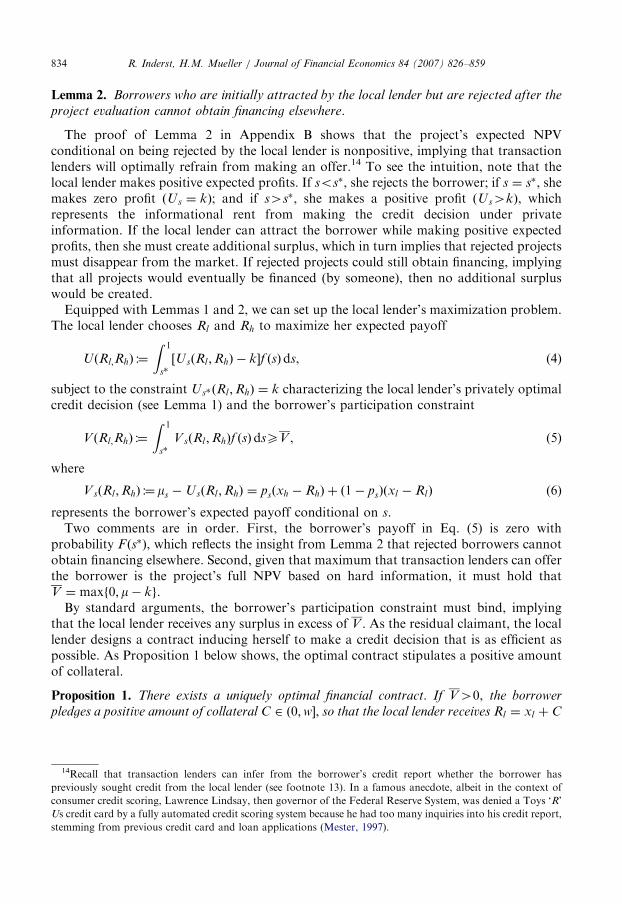
Lemma 2. Borrowers who are initially attracted by the local lender but are rejected after the
project evaluation cannot obtain financing elsewhere.
The proof of Lemma 2 in Appendix B shows that the project’s expected NPVconditional on being rejected by the local lender is nonpositive, implying that transactionlenders will optimally refrain from making an offer.14 To see the intuition, note that thelocal lender makes positive expected profits. If sos�, she rejects the borrower; if s ¼ s�, shemakes zero profit ðUs ¼ kÞ; and if s4s�, she makes a positive profit ðUs4kÞ, whichrepresents the informational rent from making the credit decision under privateinformation. If the local lender can attract the borrower while making positive expectedprofits, then she must create additional surplus, which in turn implies that rejected projectsmust disappear from the market. If rejected projects could still obtain financing, implyingthat all projects would eventually be financed (by someone), then no additional surpluswould be created.Equipped with Lemmas 1 and 2, we can set up the local lender’s maximization problem.
The local lender chooses Rl and Rh to maximize her expected payoff
UðRl;RhÞ :¼
Z 1
s�½UsðRl ;RhÞ � k�f ðsÞds, (4)
subject to the constraint Us�ðRl ;RhÞ ¼ k characterizing the local lender’s privately optimalcredit decision (see Lemma 1) and the borrower’s participation constraint
V ðRl;RhÞ :¼
Z 1
s�V sðRl ;RhÞf ðsÞdsXV , (5)
where
V sðRl ;RhÞ :¼ms �UsðRl ;RhÞ ¼ psðxh � RhÞ þ ð1� psÞðxl � RlÞ (6)
represents the borrower’s expected payoff conditional on s.Two comments are in order. First, the borrower’s payoff in Eq. (5) is zero with
probability F ðs�Þ, which reflects the insight from Lemma 2 that rejected borrowers cannotobtain financing elsewhere. Second, given that maximum that transaction lenders can offerthe borrower is the project’s full NPV based on hard information, it must hold thatV ¼ maxf0; m� kg.By standard arguments, the borrower’s participation constraint must bind, implying
that the local lender receives any surplus in excess of V . As the residual claimant, the locallender designs a contract inducing herself to make a credit decision that is as efficient aspossible. As Proposition 1 below shows, the optimal contract stipulates a positive amountof collateral.
Proposition 1. There exists a uniquely optimal financial contract. If V40, the borrower
pledges a positive amount of collateral C 2 ð0;w�, so that the local lender receives Rl ¼ xl þ C
14Recall that transaction lenders can infer from the borrower’s credit report whether the borrower has
previously sought credit from the local lender (see footnote 13). In a famous anecdote, albeit in the context of
consumer credit scoring, Lawrence Lindsay, then governor of the Federal Reserve System, was denied a Toys ‘R’
Us credit card by a fully automated credit scoring system because he had too many inquiries into his credit report,
stemming from previous credit card and loan applications (Mester, 1997).

ARTICLE IN PRESSR. Inderst, H.M. Mueller / Journal of Financial Economics 84 (2007) 826–859 835
in the bad state and Rh 2 ðRl ;xhÞ in the good state. If V ¼ 0, the local lender receives the full
project cash flow, that is, Rl ¼ xl and Rh ¼ xh.15
The case where V ¼ 0 is special, arising only because we assumed that the local lenderhas all of the bargaining power. If the borrower had positive bargaining power, we wouldhave V40 even if the borrower’s outside option were zero, that is, even if m� kp0(see Section 4.1). Clearly, if V ¼ 0, there is no role for collateral. The local lender can thenextract the full project cash flow, which implies that her credit decision is first-best optimal.
The interesting case is that in which V40. The local lender then cannot extract the fullproject cash flow, implying that her expected payoff UsðRl ;RhÞ is less than the expectedproject cash flow ms for all s 2 ½0; 1�. In particular, it holds that UsFB
ðRl ;RhÞomsFB¼ k,
that is, the local lender does not break even at s ¼ sFB. As UsðRl ;RhÞ strictly increases in s,this implies that s�4sFB, that is, the local lender’s privately optimal cutoff exceeds the first-best cutoff. In other words, the local lender rejects projects with a low but positive NPV.
Collateral can mitigate the inefficiency. Collateral should optimally be added when theproject’s cash flow is low, not when it is high, implying that Rl4xl . This improves the locallender’s payoff primarily from low-NPV projects, and thus from precisely those projectsthat she inefficiently rejects. By contrast, adding collateral when the project’s cash flow ishigh, that is, when Rh4xh, would improve the local lender’s payoff primarily from high-NPV projects that are accepted anyway. It is therefore optimal to flatten the local lender’spayoff function by adding collateral in the bad state, thereby increasing Rl , and bysimultaneously decreasing Rh to satisfy the borrower’s participation constraint. Arguably,the two payoff adjustments have opposite effects on the local lender’s cutoff s�. IncreasingRl pushes s� down, and thus closer to sFB, while decreasing Rh drags s� away from sFB. Andyet, the overall effect is that s� is pushed down.
To see why s� must be pushed down, suppose that the local lender’s optimal cutoff iscurrently s� ¼ s, and suppose that the local lender increases Rl and simultaneouslydecreases Rh such that, conditional on sXs, the borrower’s expected payoffR 1
sVsðRl ;RhÞf ðsÞds remains unchanged. While on average, that is, over the interval ½s; 1�,
the borrower remains equally well off, his conditional expected payoff VsðRl ;RhÞ is higherat high values of s 2 ½s; 1� and lower at low values of s 2 ½s; 1�. The opposite holds for thelocal lender. Her conditional expected payoff UsðRl ;RhÞ is now higher at low values ofs 2 ½s; 1� and lower at high values of s 2 ½s; 1�. Consequently, the local lender’s payofffunction has flattened over the interval ½s; 1�. Most important, her conditional expectedpayoff UsðRl ;RhÞ is now greater than k at s ¼ s, which implies that s is no longer theoptimal cutoff. As UsðRl ;RhÞ is strictly increasing in s, the (new) optimal cutoff must belower than s, implying that s� is pushed down.16
Similar to the effect on the local lender’s optimal cutoff s�, when viewed in isolation, theincrease in Rl and simultaneous decrease in Rh have opposite effects on the local lender’s
15The optimal repayment Rh in the good state if V40 is uniquely determined by the borrower’s binding
participation constraint Eq. (5) after inserting Rl ¼ xl þ C. In case of indifference, we stipulate that repayments
are first made out of the project’s cash flow.16The proof of Proposition 1 in Appendix B shows that the increase in Rl and simultaneous decrease in Rh
discussed here is feasible, that is, it does not violate the borrower’s participation constraint. In fact, both the local
lender and the borrower are strictly better off when the optimal cutoff is pushed down. The local lender can
therefore, in a final step, increase Rh further, thus pushing the optimal cutoff even further down, until the
borrower’s participation constraint binds.

ARTICLE IN PRESSR. Inderst, H.M. Mueller / Journal of Financial Economics 84 (2007) 826–859836
profit. The overall effect, however, is that the local lender’s profit increases. Intuitively,that s� is pushed down toward sFB implies that additional surplus is created. As theborrower’s participation constraint holds with equality, this additional surplus accrues tothe local lender.For convenience, let us write the optimal repayment in the good state in terms of an
optimal loan rate r, where Rh :¼ð1þ rÞk. As the risk-free interest rate is normalized to zero,the loan rate also represents the required risk premium. By Proposition 1, the optimalcontract is then fully characterized by two variables, r and C.
3.3. Optimal credit decision and financial contract as a function of pledgeable assets
Proposition 1 qualitatively characterizes the optimal contract. It remains to derive thespecific solution to the local lender’s maximization problem, that is, the specific optimalloan rate and collateral as a function of the borrower’s pledgeable assets w. If V ¼ 0, thefirst best can be trivially attained without the help of collateral. In what follows, we focuson the nontrivial case V40.There are two subcases. If the borrower has insufficient pledgeable assets to attain the
first best, then the uniquely optimal contract stipulates that he pledges all of his assets ascollateral. If the borrower has sufficient pledgeable assets, then there exist unique valuesCFB and rFB, which are jointly determined by the borrower’s binding participationconstraint Eq. (5) with V ¼ m� k and the condition that
psFBð1þ rFBÞk þ ð1� psFB
Þðxl þ CFBÞ ¼ k, (7)
where psFBis defined in Eq. (1). Solving these two equations yields unique values
CFB ¼ðk � xlÞðm� kÞR 1
sFBðms � kÞf ðsÞds
(8)
and
rFB ¼1
kxh � CFB
xh � k
k � xl
� �� 1. (9)
We obtain the following result.
Proposition 2. If the borrower has sufficient pledgeable assets wXCFB, then the first best can
be implemented with the uniquely optimal financial contract ðrFB;CFBÞ defined in Eqs. (8) and(9). If woCFB, the local lender’s credit decision is inefficient; she rejects projects with a low
but positive NPV. The uniquely optimal financial contract then stipulates that the borrower
pledges all of his assets as collateral, that is, C ¼ w.17
Proposition 2 shows that there is a natural limit to how flat the local lender’s payofffunction should optimally be. Even in the ideal case in which the borrower has sufficientpledgeable assets to attain the first best, the local lender’s payoff function will not be
17The optimal loan rate r :¼Rh=k � 1 in case woCFB is uniquely determined by the borrower’s binding
participation constraint Eq. (5) after inserting Rl ¼ xl þ w.
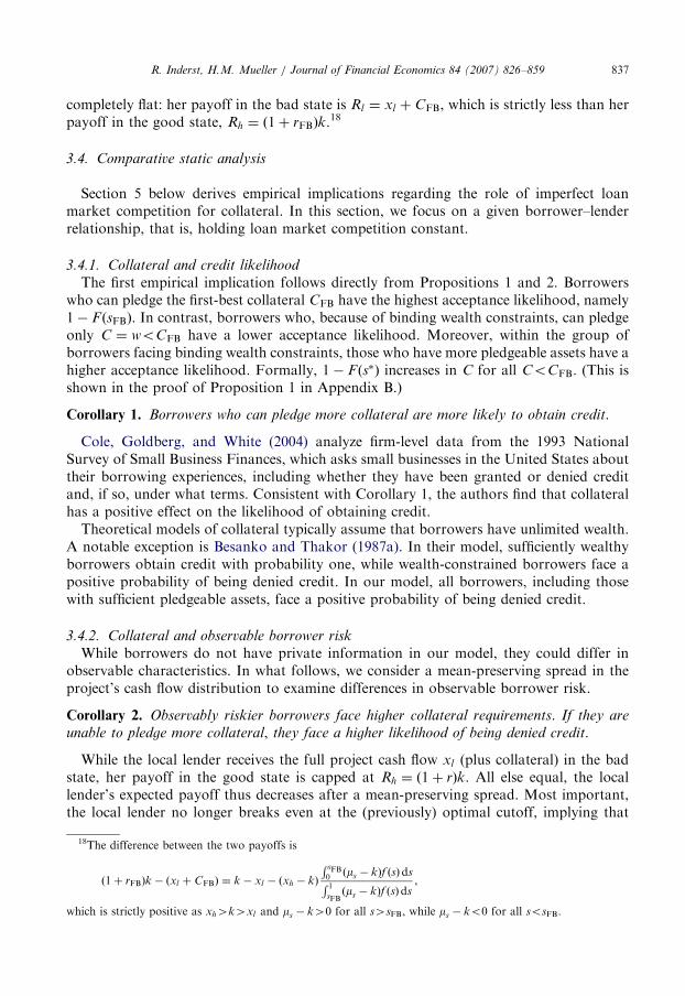
ARTICLE IN PRESSR. Inderst, H.M. Mueller / Journal of Financial Economics 84 (2007) 826–859 837
completely flat: her payoff in the bad state is Rl ¼ xl þ CFB, which is strictly less than herpayoff in the good state, Rh ¼ ð1þ rFBÞk.
18
3.4. Comparative static analysis
Section 5 below derives empirical implications regarding the role of imperfect loanmarket competition for collateral. In this section, we focus on a given borrower–lenderrelationship, that is, holding loan market competition constant.
3.4.1. Collateral and credit likelihood
The first empirical implication follows directly from Propositions 1 and 2. Borrowerswho can pledge the first-best collateral CFB have the highest acceptance likelihood, namely1� F ðsFBÞ. In contrast, borrowers who, because of binding wealth constraints, can pledgeonly C ¼ woCFB have a lower acceptance likelihood. Moreover, within the group ofborrowers facing binding wealth constraints, those who have more pledgeable assets have ahigher acceptance likelihood. Formally, 1� F ðs�Þ increases in C for all CoCFB. (This isshown in the proof of Proposition 1 in Appendix B.)
Corollary 1. Borrowers who can pledge more collateral are more likely to obtain credit.
Cole, Goldberg, and White (2004) analyze firm-level data from the 1993 NationalSurvey of Small Business Finances, which asks small businesses in the United States abouttheir borrowing experiences, including whether they have been granted or denied creditand, if so, under what terms. Consistent with Corollary 1, the authors find that collateralhas a positive effect on the likelihood of obtaining credit.
Theoretical models of collateral typically assume that borrowers have unlimited wealth.A notable exception is Besanko and Thakor (1987a). In their model, sufficiently wealthyborrowers obtain credit with probability one, while wealth-constrained borrowers face apositive probability of being denied credit. In our model, all borrowers, including thosewith sufficient pledgeable assets, face a positive probability of being denied credit.
3.4.2. Collateral and observable borrower risk
While borrowers do not have private information in our model, they could differ inobservable characteristics. In what follows, we consider a mean-preserving spread in theproject’s cash flow distribution to examine differences in observable borrower risk.
Corollary 2. Observably riskier borrowers face higher collateral requirements. If they are
unable to pledge more collateral, they face a higher likelihood of being denied credit.
While the local lender receives the full project cash flow xl (plus collateral) in the badstate, her payoff in the good state is capped at Rh ¼ ð1þ rÞk. All else equal, the locallender’s expected payoff thus decreases after a mean-preserving spread. Most important,the local lender no longer breaks even at the (previously) optimal cutoff, implying that
18The difference between the two payoffs is
ð1þ rFBÞk � ðxl þ CFBÞ ¼ k � xl � ðxh � kÞ
R sFB0 ðms � kÞf ðsÞdsR 1sFBðms � kÞf ðsÞds
,
which is strictly positive as xh4k4xl and ms � k40 for all s4sFB, while ms � ko0 for all sosFB.

ARTICLE IN PRESSR. Inderst, H.M. Mueller / Journal of Financial Economics 84 (2007) 826–859838
without any adjustment of the loan terms, the optimal cutoff must increase. By the samelogic as in Propositions 1 and 2, the local lender consequently raises the collateralrequirement.Given the difficulty of finding a good proxy for observable borrower risk, empirical
studies have employed a variety of different proxies. And yet, all of the studies find apositive relation between observable borrower risk and loan collateralization (Leeth andScott, 1989; Berger and Udell, 1995; Dennis, Nandy, and Sharpe, 2000; Jimenez, Salas, andSaurina, 2006a). To our knowledge, Boot, Thakor, and Udell (1991) are the only othermodel of collateral that considers variations in observable borrower risk. They, too, findthat observably riskier borrowers may pledge more collateral and, moreover, thatcollateralized loans may be riskier ex post.
3.4.3. Collateral and ex post default likelihood
That observably riskier borrowers pledge more collateral already implies thatcollateralized loans have a higher ex post default likelihood. However, this predictionfollows from our model even if we control for observable borrower risk. In our model, theaverage default likelihood among accepted borrowers under a lenient credit policy (low s�)is higher than it is under a conservative credit policy (high s�). Formally, the averagedefault likelihood conditional on the borrower being accepted is
D :¼
Z 1
s�ð1� psÞ
f ðsÞ
1� F ðs�Þds, (10)
where f ðsÞ=½1� F ðs�Þ� is the density of s conditional on sXs�. Given that 1� ps isdecreasing in s, and given that s� is decreasing in the amount of collateral, an increase incollateral thus implies a higher average default likelihood of accepted borrowers.
Corollary 3. Controlling for observable borrower risk, collateralized loans are more likely to
default ex post.
Corollary 3 is consistent with empirical evidence by Jimenez and Saurina (2004) andJimenez, Salas, and Saurina (2006a), who find that, controlling for observable borrowerrisk, collateralized loans have a higher probability of default in the year after the loan wasgranted. Similarly, Berger and Udell (1990), using past dues and nonaccruals to proxy fordefault risk, find that collateralized loans are riskier ex post.With the exception of Boot, Thakor, and Udell (1991), existing models of collateral
generally predict that collateralized loans are safer, not riskier. In adverse selection models(Bester, 1985; Chan and Kanatas, 1985; Besanko and Thakor, 1987a,b), this is because safeborrowers reveal their type by posting collateral. In moral-hazard models (Chan andThakor, 1987; Boot and Thakor, 1994), it is because collateral improves the incentives ofborrowers to work hard, which reduces their default likelihood.
4. Robustness
Thus far, we have assumed that the local lender has all of the ex ante bargaining power.Moreover, it has been assumed that the local lender’s decision to reject the borrower is notsubject to renegotiations. In this section, we show that our results are robust to allowingfor bargaining at both the ex ante and interim stage.
ARTICLE IN PRESSR. Inderst, H.M. Mueller / Journal of Financial Economics 84 (2007) 826–859 839
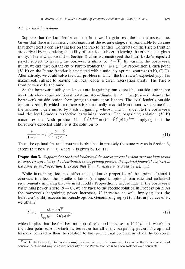
4.1. Ex ante bargaining
Suppose that the local lender and the borrower bargain over the loan terms ex ante.Given that there is symmetric information at the ex ante stage, it is reasonable to assumethat they select a contract that lies on the Pareto frontier. Contracts on the Pareto frontierare derived by maximizing the utility of one side, subject to leaving the other side a givenutility. This is what we did in Section 3 when we maximized the local lender’s expectedpayoff subject to leaving the borrower a utility of V ¼ V . By varying the borrower’sutility, we can trace out the entire Pareto frontier U ¼ uðV Þ.19 By Proposition 1, each pointðU ;V Þ on the Pareto frontier is associated with a uniquely optimal contract ðrðV Þ;CðV ÞÞ.Alternatively, we could solve the dual problem in which the borrower’s expected payoff ismaximized, subject to leaving the local lender a given reservation utility. The Paretofrontier would be the same.
As the borrower’s utility under ex ante bargaining can exceed his outside option, we
must introduce some additional notation. Accordingly, let V ¼ maxf0; m� kg denote theborrower’s outside option from going to transaction lenders. The local lender’s outsideoption is zero. Provided that there exists a mutually acceptable contract, we assume thatthe solution is determined by Nash bargaining, where b and 1� b denote the borrower’sand the local lender’s respective bargaining powers. The bargaining solution ðU ;V Þ
maximizes the Nash product ðV � V ÞbU1�b ¼ ðV � V Þb½uðV Þ�1�b, implying that theborrower’s expected utility V is the solution to
b
1� b¼ �u0ðV Þ
V � V
uðV Þ. (11)
Thus, the optimal financial contract is obtained in precisely the same way as in Section 3,
except that now V ¼ V , where V is given by Eq. (11).
Proposition 3. Suppose that the local lender and the borrower can bargain over the loan terms
ex ante. Irrespective of the distribution of bargaining powers, the optimal financial contract is
the same as in Proposition 1, except that V ¼ V , where V is given by Eq. (11).
While bargaining does not affect the qualitative properties of the optimal financialcontract, it affects the specific solution (the specific optimal loan rate and collateralrequirement), implying that we must modify Proposition 2 accordingly. If the borrower’sbargaining power is zero ðb! 0Þ, we are back to the specific solution in Proposition 2. Asthe borrower’s bargaining power increases, V increases as well, implying that theborrower’s utility exceeds his outside option. Generalizing Eq. (8) to arbitrary values of V ,we obtain
CFB :¼ðk � xlÞVR 1
sFBðms � kÞf ðsÞds
, (12)
which implies that the first-best amount of collateral increases in V . If b! 1, we obtainthe other polar case in which the borrower has all of the bargaining power. The optimalfinancial contract is then the solution to the specific dual problem in which the borrower
19While the Pareto frontier is decreasing by construction, it is convenient to assume that it is smooth and
concave. A standard way to ensure concavity of the Pareto frontier is to allow lotteries over contracts.

ARTICLE IN PRESSR. Inderst, H.M. Mueller / Journal of Financial Economics 84 (2007) 826–859840
makes a take-it-or-leave-it offer that maximizes his expected payoff, subject to leaving thelocal lender a reservation utility of zero. The local lender’s participation constraint in thiscase is slack. As the local lender makes her credit decision under private information, shecan always extract an informational rent (see Section 3.2). This is different from models inwhich the agency problem lies with the borrower. In such models, if the borrower has all ofthe bargaining power or the loan market is perfectly competitive, lenders generally makezero profits.
4.2. Interim bargaining
We now reconsider our assumption that the local lender’s decision to reject the borroweris final and not subject to renegotiations. Clearly, if the borrower could observe the locallender’s project evaluation, any inefficiency would be renegotiated away. If s 2 ½sFB; s�Þ, thelocal lender and the borrower would simply change the loan terms to allow the local lenderto break even. Given that the borrower cannot observe the local lender’s project evaluationhowever, such a mutually beneficial outcome may not arise. In fact, as we will now show,the original loan terms will not be renegotiated in equilibrium.Consider the following simple renegotiation game. After the local lender has evaluated
the borrower’s project, either she or the borrower can make a take-it-or-leave-it offer toreplace the original loans terms with new ones.20 If the local lender makes the offer, theborrower must agree; if the borrower makes the offer, the local lender must agree. If thetwo cannot agree, the original loan terms remain in place.
Proposition 4. Suppose that the local lender and the borrower can renegotiate the original
loan terms after the local lender’s project evaluation. Regardless of who makes the contract
offer at the interim stage, the original loan terms remain in place.
The intuition is straightforward. As only the local lender can observe s, the borrowerdoes not know whether sos� or sXs�. In the first case, adjusting the loan terms mightallow the local lender to break even, avoiding an inefficient rejection. However, in thesecond case, the local lender would have accepted the project anyway. Adjusting the loanterms would then merely constitute a wealth transfer to the local lender. By Proposition 4,the expected value to the borrower from adjusting the loan terms, given that he does notknow whether sos� or sXs�, is negative.Finally, we ask whether it might ever be suboptimal to set the loan terms ex ante. That
is, would the local lender ever prefer to wait until after the project evaluation?21 Theanswer is no. Suppose that the local lender waits until after the project evaluation. In thiscase, any equilibrium of the signaling game in which the borrower is attracted mustprovide the borrower an expected utility of at least V . Moreover, while waiting allows thelocal lender to fine-tune her offer to the outcome of the project evaluation, she canaccomplish the same by offering an incentive-compatible menu of contracts ex ante fromwhich she chooses at the interim stage. It is easy to show that offering such a menu is
20To the best of our knowledge, there exists no suitable axiomatic bargaining concept a la Nash bargaining to
analyze surplus sharing under private information, hence the restriction to the two polar cases in which either the
borrower or the local lender makes a take-it-or-leave-it offer. Our results would be the same if the local lender and
the borrower could make alternating offers, as long as there is no additional sorting variable.21As the borrower’s information remains the same, he would make the same offer in t ¼ 0 and 1.

ARTICLE IN PRESSR. Inderst, H.M. Mueller / Journal of Financial Economics 84 (2007) 826–859 841
suboptimal in our model.22 Consequently, the local lender does not benefit from waitingwith her offer until after the project evaluation.
5. Imperfect loan market competition and collateral
Thus far we have focused on a given borrower–lender relationship, holding loan marketcompetition constant. We now consider changes in loan market competition, examininghow advances in information technology that increase the competitive pressure fromtransaction lenders affect loan rates and collateral requirements.
5.1. Changes in the local lender’s information advantage
One implication of the information revolution in small business lending (seeIntroduction) is that the information advantage of local lenders has narrowed. This isespecially true since the 1990s, when small business credit scoring was adopted on a broadscale in the United States.23 Small business credit scoring models fairly accurately predictthe likelihood that a borrower will default based solely on hard information, especiallycredit reports, thus reducing the information uncertainty associated with small businessloans made to borrowers located far away.24
To obtain a continuous yet simple measure of the local lender’s information advantagevis-a-vis transaction lenders, we assume that it is now only with probability 0oqp1 thatthe local lender has a better estimate of the project’s success probability. Our base modelcorresponds to the case in which q ¼ 1. As in our base model, we assume that only the locallender can observe her own success probability estimate. We obtain the following result.
Proposition 5. There exists a threshold bq such that borrowers for whom the local lender’sinformation advantage is large ðqXbqÞ go to the local lender, while borrowers for whom the
local lender’s information advantage is small ðqobqÞ borrow from transaction lenders.Conditional on going to the local lender ðqXbqÞ, borrowers for whom the local lender’s
information advantage is relatively smaller (lower q) face lower loan rates but higher
collateral requirements.
Why is a small but positive information advantage not already sufficient to attract theborrower?25 As in our base model, borrowers who are rejected by the local lender areunable to obtain financing elsewhere. Hence, from the borrower’s perspective, going to thelocal lender and being rejected is worse than borrowing directly from transaction lenders.
22Intuitively, allowing the local lender to choose from a menu after the project evaluation creates a ‘‘self-dealing
problem,’’ as the local lender always picks the contract that is ex post optimal for her. This makes it more difficult
to satisfy the borrower’s participation constraint, implying that the local lender’s privately optimal cutoff s� is
higher (and thus less efficient) than under the single optimal contract from Proposition 2.23The first bank in the United States to adopt small business credit scoring was Wells Fargo in 1993, using a
proprietary credit scoring model. Already in 1997, only two years after Fair, Isaac & Co. introduced the first
commercially available small business credit-scoring model, 70% of the (mainly large) banks surveyed in the
Federal Reserve’s Senior Loan Officer Opinion Survey responded that they use credit scoring in their small
business lending (Mester, 1997).24Frame et al. (2001, p. 813) conclude: ‘‘[C]redit scoring lowers information costs between borrowers and
lenders, thereby reducing the value of traditional, local bank lending relationships.’’25The threshold bq in Proposition 5 may not always lie strictly between zero and one. For instance, if m� kp0,
the borrower’s outside option is zero, implying that the local lender can attract the borrower for any q40.

ARTICLE IN PRESSR. Inderst, H.M. Mueller / Journal of Financial Economics 84 (2007) 826–859842
To attract the borrower, the local lender must therefore offer him a loan rate that is belowthe rate offered by transaction lenders, which implies that the local lender must createadditional surplus. But merely creating some additional surplus is not enough. As the locallender extracts an informational rent (see Section 3.2), she can promise only a fraction ofthe created surplus to the borrower, implying that, to attract the borrower, the additionalsurplus created must be sufficiently large. That is, q must be sufficiently high.Before we link Proposition 5 to advances in information technology narrowing the local
lender’s information advantage, it is worth pointing out that the proposition has cross-sectional implications. Borrowers who borrow locally ðqXbqÞ and for whom the locallender’s information advantage is relatively smaller (lower q) face lower loan rates buthigher collateral requirements. Intuitively, a decrease in q implies that the local lendercreates less surplus by screening out negative-NPV projects. Holding the loan rateconstant, a decrease in q therefore reduces the borrower’s expected payoff, violating his(previously binding) participation constraint. To attract the borrower, the local lendermust consequently offer a lower loan rate. But a lower loan rate implies that the borrowerreceives a larger share of the project’s cash flow, which in turn implies that the local lendermust raise the collateral requirement to minimize distortions in her credit decision.As the sole role of collateral in our model is to minimize distortions in credit decisions
based on soft information, collateral has no meaningful role to play in loans underwrittenby transaction lenders. Indeed, while the vast majority of small business loans in theUnited States are collateralized (Avery, Bostic, and Samolyk 1998; Berger and Udell,1998), small business loans made by transaction lenders on the basis of credit scoring aregenerally unsecured (Zuckerman, 1996; Frame, Srinivasan, and Woosley, 2001; Frame,Padhi, and Woosley, 2004). Our model also predicts that, within the group of borrowerswho borrow locally, loans should be more collateralized when the local lender’sinformation advantage is smaller. Consistent with this prediction, Petersen and Rajan(2002) find that small business borrowers who are located farther away from their locallender are more likely to pledge collateral. Proposition 5 is also consistent with evidence byBerger and Udell (1995) and Degryse and van Cayseele (2000), who both find that longerborrower relationships are associated with less collateral.26
We can alternatively interpret Proposition 5 as a change in the local lender’s informationadvantage for any given borrower. With the widespread adoption of small business creditscoring since the 1990s, this information advantage has narrowed. According toProposition 5, a narrowing of the local lender’s information advantage has two effects.First, marginal borrowers for whom the local lender has only a small informationadvantage will switch to transaction lenders. Various studies show that transaction lendersusing small business credit scoring have successfully expanded their small business lendingto borrowers outside of their own markets (Hannan, 2003; Frame, Padhi, and Woosley,2004; Berger, Frame, and Miller, 2005).27 Second, borrowers who continue to borrow from
26These findings are consistent with our model to the extent that the local lender’s information advantage
increases with the length of borrower relationships. They are also consistent with Boot and Thakor (1994), who
model relationship lending as a repeated game, showing that collateral decreases with the duration of borrower
relationships.27Berger and Frame (2007, p. 15) argue: ‘‘[T]echnological change—including the introduction of SBCS [small
business credit scoring]—may have increased the competition for small business customers and potentially
widened the geographic area over which these firms may search for credit. Presumably, a small business with an
acceptable credit score could now shop nationwide through the Internet among lenders using SBCS.’’

ARTICLE IN PRESSR. Inderst, H.M. Mueller / Journal of Financial Economics 84 (2007) 826–859 843
their local lender will face lower loan rates but higher collateral requirements. We areunaware of empirical studies examining how the adoption of small business credit scoringhas affected the loan terms in local lending relationships.
5.2. Changes in the costs of transaction lending
A second, and perhaps more immediate, implication of the information revolution insmall business lending is that the costs of underwriting transaction loans have decreased.Processing costs for small business loans based on credit scoring have decreasedconsiderably (Mester, 1997), input databases for credit scoring models have becomelarger, and credit reports can nowadays be sent at relatively low costs over the internet(DeYoung, Hunter, and Udell, 2004; Berger and Frame, 2007).28
To examine the implications of a decrease in the costs of transaction lending, we assumethat underwriting a transaction loan involves a cost of k. As the market for transactionloans is perfectly competitive, this cost is ultimately borne by the borrower, implying thatthe borrower’s outside option from going to transaction lenders is V ¼ maxf0;m� k � kg.If V ¼ 0, a change in k has no effect in our model. In the following, we thus focus on thenontrivial case in which V ¼ m� k � k40.
As in the case of a decrease in q, a decrease in the costs of transaction lending impliesthat the local lender loses marginal borrowers to transaction lenders. This is precisely whatBoot and Thakor (2000) show in their analysis of loan market competition betweentransaction lenders and relationship lenders. What is less clear is to what extent a decreasein the costs of transaction lending affects collateral requirements. We obtain the followingresult.
Proposition 6. A decrease in the costs of transaction lending (lower k) forces the local lender
to lower the loan rate and to increase the collateral requirement. The increase in collateral
requirement for a given decrease in k is greater for borrowers for whom the local lender has a
relatively smaller information advantage (lower q).
A decrease in the costs of transaction lending increases the value of the borrower’soutside option, thus increasing the competitive pressure from transaction lenders. Toattract the borrower, the local lender must consequently lower the loan rate. As in the caseof a narrowing of the local lender’s information advantage, this implies that the locallender must raise the collateral requirement to minimize distortions in her credit decision.The increase in collateral requirement is greater for borrowers for whom the local lenderhas a relatively smaller information advantage. The intuition is the same as that for whythese borrowers face higher collateral requirements in the first place (see Proposition 5).
We are unaware of empirical studies investigating how changes in the costs oftransaction lending affect the use of collateral in small business loans. There is, however,evidence that the use of collateral increases with loan market competition, which isconsistent with Proposition 6. Using Spanish data, Jimenez and Saurina (2004) andJimenez, Salas, and Saurina (2006a) show a positive relation between collateral andbank competition, as measured by the Herfindahl index. Moreover, Jimenez, Salas,and Saurina (2006b) find that the positive effect of bank competition on collateral
28At the same time, there appears to be little evidence that advances in information technology had a significant
direct impact on relationship lending (DeYoung et al., 2004).

ARTICLE IN PRESSR. Inderst, H.M. Mueller / Journal of Financial Economics 84 (2007) 826–859844
decreases with the length of borrower relationships, which is consistent with our argumentif the local lender’s information advantage increases with the duration of borrowerrelationships.To our knowledge, related models of imperfect loan market competition (Boot and
Thakor, 2000; Hauswald and Marquez, 2003, 2006) do not consider collateral. On theother hand, theoretical models of collateral do not consider imperfect loan marketcompetition between arm’s-length transaction lenders and local relationship lenders, thusgenerating empirical predictions that are different from ours. For instance, Besanko andThakor (1987a) and Manove, Padilla, and Pagano (2001) both find that collateral is usedin a perfectly competitive loan market, but not in a monopolistic one. Closer in spirit toour model, Villas-Boas and Schmidt-Mohr (1999) consider an oligopolistic loan marketwith horizontally differentiated banks, showing that collateral could either increase ordecrease as bank competition increases.
6. Conclusion
This paper offers a novel argument for collateral based on the notion that collateralmitigates distortions in credit decisions based on soft information. Our argument isentirely lender-based. There is no borrower moral hazard or adverse selection.In our model, there is a local relationship lender who has access to soft private
information, allowing her to estimate the borrower’s default likelihood more precisely thancan transaction lenders, who provide arm’s-length financing based on publicly availableinformation. While the local lender has a competitive advantage, competition fromtransaction lenders provides the borrower with a positive outside option that the locallender must match. To attract the borrower, the local lender must leave him some of thesurplus from the project, which distorts her credit decision, with the effect that she rejectsmarginally profitable projects. Collateral improves the local lender’s payoff from projectswith a relatively high likelihood of low cash flows, and thus from precisely those projectsthat she inefficiently rejects.That the local lender’s credit decision is based on soft and private information is crucial
for the inefficiency studied here, and hence for our argument for collateral. If theinformation were observable and contractible, the local lender could contractually committo the first-best credit decision even if it meant committing to a decision rule that is ex postsuboptimal. Likewise, if the information were observable but nonverifiable, the inefficiencycould be eliminated through bargaining at the interim stage.Given that our model is cast as an imperfectly competitive loan market in which a local
lender has an information advantage vis-a-vis transaction lenders, we can drawimplications regarding the effects of technological innovations that increase thecompetitive pressure from transaction lenders. We find that technological innovationsthat narrow the information advantage of local lenders, such as small business creditscoring, lead to lower loan rates but higher collateral requirements (Proposition 5).Likewise, innovations that lower the costs of underwriting transaction loans lead to greatercompetition from transaction lenders, lower loan rates, and higher collateral requirements(Proposition 6). Moreover, the increase in collateral requirements is greater for borrowersfor whom the local lender has a weaker information advantage, such as borrowers who arelocated farther away from the local lender, or borrowers with whom the local lender has noprior lending relationship (Proposition 6).

ARTICLE IN PRESSR. Inderst, H.M. Mueller / Journal of Financial Economics 84 (2007) 826–859 845
In addition to generating empirical implications regarding loan market competition, ourmodel also has implications for a given borrower–lender relationship, holding loan marketcompetition constant. We find that borrowers who can pledge more collateral are morelikely to obtain credit (Corollary 1), that observably riskier borrowers face highercollateral requirements (Corollary 2), and that, controlling for observable borrower risk,collateralized loans are more likely to default ex post (Corollary 3). All three predictionsare borne out in the data. What is more, existing models of collateral, with the exception ofBoot, Thakor, and Udell (1991), generally make the opposite prediction, namely, thatcollateralized loans are safer, not riskier.
Appendix A. Continuum of cash flows
This section shows that our argument for why collateral is optimal extends to a continuumof cash flows. Unlike the two cash flow model in the main text, it shows both that collateral isused only in low cash flow states and how precisely repayments are made out of the pledgedassets as a function of the project’s cash flow when cash flows are continuous.
We assume that the project cash flow x is distributed with atomless distribution functionGsðxÞ over the support X :¼ ½0;x�, where x40 may be finite or infinite. The density gsðxÞ iseverywhere continuous and positive. In case x is infinite, we assume that ms :¼
RX
xgsðxÞdx
exists for all s 2 ½0; 1�. We moreover assume that GsðxÞ satisfies the monotone likelihoodratio property (MLRP), which states that for any pair ðs; s0Þ 2 S with s04s, the ratiogs0 ðxÞ=gsðxÞ strictly increases in x for all x 2 X .
A financial contract specifies a repayment schedule tðxÞpx out of the project’s cash flow,an amount Cpw of collateral, and a repayment schedule cðxÞpC out of the pledged assets.It is convenient to write RðxÞ :¼ tðxÞ þ cðxÞ. We make the standard assumption that RðxÞ isnondecreasing for all x 2 X (e.g., Innes, 1990). The local lender’s and borrower’s expectedpayoffs are UsðRÞ :¼
RX
RðxÞgsðxÞdx, V sðRÞ :¼ms �UsðRÞ, UðRÞ :¼R 1
s�½UsðRÞ � k�f ðsÞds,
and V ðRÞ :¼R 1
s�V sðRÞf ðsÞds, respectively. Analogous to the analysis in the main text, the
local lender’s privately optimal cutoff s� is given by Us�ðRÞðRÞ ¼ k. The local lender’sproblem is to maximize UðRÞ, subject to the borrower’s participation constraint V ðRÞXV .
The following result extends Proposition 1 to the case with a continuum of cash flows.
Proposition. The optimal financial contract when there is a continuum of cash flows stipulates
a repayment R 2 ð0;xÞ and an amount of collateral C 2 ð0;w�, so that the local lender
receives RðxÞ ¼ xþ C if xpR and RðxÞ ¼ R if x4R.
As far as the repayment out of the project’s cash flow is concerned, we have tðxÞ ¼ x forxpR and tðxÞ ¼ R for x4R. Collateral is used as follows: if xpR� C, the local lenderreceives the entire collateral, that is, cðxÞ ¼ C; if R� CoxpR, the local lender receives afraction cðxÞ ¼ R� x of the pledged assets (after liquidation); and if x4R, the local lenderreceives no repayment out of the pledged assets, because the project’s cash flow is sufficientto make the contractually stipulated repayment.
To prove the proposition, suppose to the contrary that the optimal contract stipulated arepayment schedule RðxÞ different from the one in the proposition. We can then constructa new repayment schedule eRðxÞ ¼ minfxþ eC; eRg, where eC ¼ w, and where eR satisfiesZ 1
s�ðRÞ
ZX
zðxÞgsðxÞdx
� �f ðsÞds ¼ 0, (13)
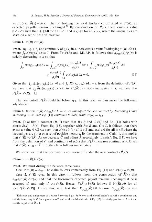
ARTICLE IN PRESSR. Inderst, H.M. Mueller / Journal of Financial Economics 84 (2007) 826–859846
with zðxÞ :¼ eRðxÞ � RðxÞ. That is, holding the local lender’s cutoff fixed at s�ðRÞ, allexpected payoffs remain unchanged.29 By construction of eRðxÞ, there exists a value0oexox such that zðxÞX0 for all xoex and zðxÞp0 for all x4ex, where the inequalities arestrict on a set of positive measure.
Claim 1. s�ð eRÞos�ðRÞ.
Proof. By Eq. (13) and continuity of gsðxÞ in s, there exists a value es satisfying s�ðRÞoeso1,where
RX
zðxÞgesðxÞdx ¼ 0. From es4s�ðRÞ and MLRP, it follows that gs�ðRÞðxÞ=gesðxÞ isstrictly decreasing in x so thatZ
X
zðxÞgs�ðRÞðxÞdx ¼
Zxpex zðxÞgesðxÞ gs�ðRÞðxÞ
gesðxÞ dxþ
Zx4ex zðxÞgesðxÞ gs�ðRÞðxÞ
gesðxÞ dx
4gs�ðRÞðexÞ
gesðexÞZ
X
zðxÞgesðxÞdx ¼ 0. ð14Þ
Given thatR
XzðxÞgs�ðRÞðxÞdx40 and
RX
RðxÞgs�ðRÞðxÞdx ¼ k from the definition of s�ðRÞ,
we have thatR
XeRðxÞgs�ðRÞðxÞdx4k. As Usð eRÞ is strictly increasing in s, we have that
s�ð eRÞos�ðRÞ. &
The new cutoff s�ð eRÞ could lie below sFB. In this case, we can make the followingadjustment.
Claim 2. In case s�ð eRÞosFB for eC ¼ w, we can adjust the new contract by decreasing eC and
increasing eR, so that Eq. (13) continues to hold, while s�ð eRÞ ¼ sFB.
Proof. Take first a contract ð bR; bCÞ such that bR4 eR and bCo eC and Eq. (13) holds withzðxÞ :¼ bRðxÞ � eRðxÞ. From Eq. (13), together with bR4 eR and bCo eC, it follows that thereexists a value 0oexox such that zðxÞX0 for all x4ex and zðxÞp0 for all xoex,where theinequalities are strict on a set of positive measure. By the argument in Claim 1, this impliesthat s�ð bRÞ4s�ð eRÞ. As we decrease bC and adjust bR accordingly to satisfy Eq. (13), we havefrom the definition of s� and continuity of gsðxÞ that s�ð bRÞ increases continuously. Giventhat s�ð bRÞ4sFB at bC ¼ 0, the claim follows immediately. &
We show next that the borrower is not worse off under the new contract ð eR; eCÞ.Claim 3. V ð eRÞXV ðRÞ.
Proof. We must distinguish between three cases.Case 1: s�ðRÞ ¼ sFB. The claim follows immediately from Eq. (13) and s�ðRÞ ¼ s�ð eRÞ.Case 2: s�ðRÞ4sFB. In this case, it follows from the construction of eRðxÞ that
sFBps�ð eRÞos�ðRÞ and that the borrower’s expected payoff remains unchanged if he is
accepted if, and only if, sXs�ðRÞ. Hence, V ð eRÞXV ðRÞ follows if V sð eRÞX0 for all
s 2 ½s�ð eRÞ; s�ðRÞ�. To see this, note first that Vs�ðeRÞð eRÞX0 because U
s�ðeRÞð eRÞ ¼ k and
29Existence and uniqueness of a value eR solving Eq. (13) follows as the local lender’s payoff is continuous and
strictly increasing in eR for a given cutoff, and as the left-hand side of Eq. (13) is strictly positive at eR ¼ x and
strictly negative at eR ¼ 0.

ARTICLE IN PRESSR. Inderst, H.M. Mueller / Journal of Financial Economics 84 (2007) 826–859 847
sFBps�ð eRÞ. It remains to show that V sð eRÞ is nondecreasing in s. Partial integration yields
Vsð eRÞ ¼ Z xeR�eC ½1� GsðxÞ�dx� eC, (15)
where MLRP implies that GsðxÞ is strictly decreasing in s for all 0oxox. By Eq. (15), this
implies that Vsð eRÞ is strictly increasing in s.
Case 3: s�ðRÞosFB. In this case, it follows from the construction of eRðxÞ that s�ð eRÞ ¼ sFB.
It remains to show that V sð eRÞp0 for all s 2 ½s�ð eRÞ; sFB�. From s�ð eRÞ ¼ sFB, implying that
UsFBð eRÞ ¼ 0, it follows that VsFB
ð eRÞ ¼ 0, while the argument in Case 2 implies that Vsð eRÞis nondecreasing in s. Together, this implies that Vsð eRÞp0 for all s 2 ½s�ð eRÞ; sFB�. &
In sum, we have constructed a new contract ð eR; eCÞ with the following characteristics:eRðxÞ ¼ minfxþ eC; eRg; Eq. (13) is satisfied; if s�ðRÞXsFB, it holds that sFBps�ð eRÞps�ðRÞ,
where s�ð eRÞos�ðRÞ if s�ðRÞ4sFB; if s�ðRÞosFB, it holds that s�ðRÞos�ð eRÞ ¼ sFB; and
V ð eRÞXV ðRÞ. The new contract satisfies the borrower’s participation constraint, while the
local lender is not worse off. In fact, she is strictly better off if s�ð eRÞas�ðRÞ, which followsimmediately from Eq. (13) and the optimality of s�. Finally, if the original contract
implements the first best, that is, if s�ð eRÞ ¼ s�ðRÞ ¼ sFB, then the repayment out of the
pledged assets is strictly lower under the new contract, that is,R 1
sFB½R
XcðxÞgsðxÞdx�
f ðsÞds4R 1
sFB½R
XecðxÞgsðxÞdx�f ðsÞds. &
Appendix B. Proofs
Proof of Lemma 2. Suppose to the contrary that the project’s NPV conditional uponrejection were positive, that is, suppose thatZ s�
0
ðms � kÞf ðsÞ
F ðs�Þds40. (16)
This immediately implies that m� k40. If the project’s unconditional NPV werenonpositive, its NPV conditional upon rejection would have to be negative. Given thattransaction lenders are perfectly competitive, a rejected borrower obtains (16) in t ¼ 1when seeking funding from transaction lenders. In t ¼ 0, the borrower’s expected payofffrom going to the local lender is consequentlyZ 1
s�½ms �UsðRl ;RhÞ�f ðsÞdsþ
Z s�
0
ðms � kÞf ðsÞds, (17)
while his payoff from going to a transaction lender is m� k40. Requiring that theexpression in Eq. (17) is equal to or greater than m� k and using the fact that m ¼R 10 msf ðsÞds yields the requirement thatZ 1
s�½UsðRl ;RhÞ � k�f ðsÞdsp0, (18)
which contradicts the fact that UsðRl ;RhÞ4k for all s4s�. &

ARTICLE IN PRESSR. Inderst, H.M. Mueller / Journal of Financial Economics 84 (2007) 826–859848
Proof of Propositions 1 and 2. It is convenient to prove the two propositions together. Asthe case in which V ¼ 0 is obvious, we focus on the nontrivial case in which V40. Tomake the dependency of s� on Rl and Rh explicit, we write s� ¼ s�ðRl ;RhÞ. The followingobservations are all obvious. First, if we increase Rl while holding Rh constant, UðRl;RhÞ
increases while s�ðRl ;RhÞ decreases. Second, if we increase Rh while holding Rl constant,UðRl ;RhÞ increases while s�ðRl ;RhÞ decreases. Third, s�ðRl ;RhÞ is continuous in both Rl
and Rh, implying that V ðRl;RhÞ and UðRl ;RhÞ are also both continuous.The following two auxiliary results simplify the analysis.
Claim 1. Take two contracts ðRl ;RhÞ and ð eRl ; eRhÞ with eRl4Rl and eRhoRh. If the local
lender’s optimal cutoff is the same under both contracts, that is, if s�ðRl ;RhÞ ¼ s�ð eRl ; eRhÞ,
then V sð eRl ; eRhÞ4VsðRl ;RhÞ for alls4s�.
Proof. Because s�ðRl ;RhÞ ¼ s�ð eRl ; eRhÞ ¼ s�, we have that Us�ð eRl ; eRhÞ ¼ Us�ðRl ;RhÞ and
therefore that V s�ð eRl ; eRhÞ ¼ Vs�ðRl ;RhÞ. Given that eRh � eRloRh � Rl and
V sð eRl ; eRhÞ � VsðRl ;RhÞ ¼ ðRl � eRlÞ þ ps½ðRh � RlÞ � ð eRh � eRlÞ�, (19)
that ps is strictly increasing in s implies that V sð eRl ; eRhÞ � VsðRl ;RhÞ must be strictly
increasing in s. In conjunction with Vs�ð eRl ; eRhÞ ¼ Vs�ðRl ;RhÞ, this implies that V sð eRl ; eRhÞ4VsðRl ;RhÞ for all s4s�. &
Claim 2. Take two contracts ðRl ;RhÞ and ð eRl ; eRhÞ, where eRl4Rl and eRlo eRhoRh satisfyZ 1
s�ðRl ;RhÞ
½Vsð eRl ; eRhÞ � V sðRl ;RhÞ�f ðsÞds ¼ 0. (20)
That is, holding the cutoff fixed at s�ðRl ;RhÞ, the borrower’s (and thus also the local lender’s)expected payoffs are the same under the two contracts. It then holds that s�ð eRl ; eRhÞos�ðRl ;RhÞ.
Proof. We can transform Eq. (20) toZ 1
s�ðRl ;RhÞ
½ps½ðRh � RlÞ � ð eRh � eRlÞ� � ð eRl � RlÞ�f ðsÞ
1� F ðs�Þds ¼ 0. (21)
As ps is strictly increasing in s and Rh � Rl4 eRh � eRl by construction, Eq. (21) implies that
ps�ðRl ;RhÞ½ðRh � RlÞ � ð eRh � eRlÞ� � ð eRl � RlÞo0, (22)
and therefore that V s�ðRl ;RhÞð eRl ; eRhÞoV s�ðRl ;RhÞ
ðRl ;RhÞ. Because Us�ðRl ;RhÞðRl ;RhÞ ¼ k from
the definition of s�ðRl ;RhÞ, this implies that Us�ðRl ;RhÞð eRl ; eRhÞ4k. As Usð eRl ; eRhÞ is strictly
increasing in s and Us�ðeRl ;
eRhÞð eRl ; eRhÞ ¼ k from the definition of s�ð eRl ; eRhÞ, this implies that
s�ð eRl ; eRhÞos�ðRl ;RhÞ. &
We now prove the claim in Proposition 1 that the optimal contract is unique and that ithas a positive amount of collateral in the low cash flow state, that is, Rl4xl , whereRl � xl 2 ð0;w�. That Rhoxh follows trivially from the borrower’s participation constraintEq. (5): if Rl4xl but RhXxh, the borrower would not break even. We prove the claim

ARTICLE IN PRESSR. Inderst, H.M. Mueller / Journal of Financial Economics 84 (2007) 826–859 849
separately for the case in which ðRl;RhÞ is first-best optimal, that is, s�ðRl ;RhÞ ¼ sFB (Case1), and the case in which ðRl;RhÞ is second-best optimal, that is, s�ðRl ;RhÞ4sFB (Case 2). InCase 2, we specifically prove that Rl ¼ xl þ w, as asserted in Proposition 2. We finallyshow that it cannot be true that s�ðRl ;RhÞosFB.
Case 1: Suppose that under the optimal contract ðRl ;RhÞ it holds that s�ðRl ;RhÞ ¼ sFB.We then have from Eqs. (1) and (3) that
k � Rl
Rh � Rl
¼k � xl
xh � xl
, (23)
which uniquely pins down Rh for a given value of Rl . As we increase Rl while decreasing Rh
to satisfy Eq. (23), we know from Claim 1 that V sðRl ;RhÞ increases for alls4s�ðRl ;RhÞ ¼ sFB. Consequently, V ðRl ;RhÞ also increases. The requirement thats�ðRl ;RhÞ ¼ sFB, in conjunction with the fact that Eq. (5) holds with equality, thus pinsdown a unique pair ðRl ;RhÞ. It remains to show that Rl4xl . If Rl ¼ xl , Eq. (23) wouldimply that Rh ¼ xh and thus that V ðRl ;RhÞ ¼ 0, violating Eq. (5). By Claim 1, any lowervalue Rloxl [together with Rh4xh to satisfy Eq. (23)] would imply an even lower value ofV ðRl ;RhÞ and therefore also violate Eq. (5).
Case 2: Suppose that under the optimal contract ðRl ;RhÞ it holds that s�ðRl ;RhÞ4sFB.We first show that, in this case, it must hold that Rl ¼ xl þ w. We argue to a contradiction
and assume that Rloxl þ w. We can then construct a new contract ð eRl ; eRhÞ with eRl4Rl
and eRlo eRhoRh that satisfies Eq. (5) and is preferred by the local lender, contradicting the
optimality of ðRl ;RhÞ. We construct ð eRl ; eRhÞ as follows. Starting from eRl ¼ Rl andeRh ¼ Rh, we continuously increase eRl and decrease eRh so that Eq. (20) in Claim 2 holds.
From Claim 2, we then know that s�ð eRl ; eRhÞos�ðRl ;RhÞ, while s�ð eRl ; eRhÞ decreases
continuously as we increase eRl and decrease eRh. We continue to increase eRl and decreaseeRh until one of the following two conditions is satisfied. Either the borrower’s wealth
constraint binds, that is, eRl ¼ xl þ w (Case 2i), or it holds that s�ð eRl ; eRhÞ ¼ sFB (Case 2ii).30
We now show that the local lender prefers ð eRl ; eRhÞ to ðRl ;RhÞ and that ð eRl ; eRhÞ satisfiesthe borrower’s participation constraint Eq. (5). The first claim is obvious. The local
lender’s expected payoff under ð eRl ; eRhÞ isZ 1
s�ðeRl ;eRhÞ
½Usð eRl ; eRhÞ � k�f ðsÞds
¼
Z s�ðRl ;RhÞ
s�ðeRl ;eRhÞ
½Usð eRl ; eRhÞ � k�f ðsÞdsþ
Z 1
s�ðRl ;RhÞ
½Usð eRl ; eRhÞ � k�f ðsÞds
4Z 1
s�ðRl ;RhÞ
UsðRl ;RhÞ � k½ �f ðsÞds, ð24Þ
which follows from s�ð eRl ; eRhÞos�ðRl ;RhÞ, the fact that ð eRl ; eRhÞ and ðRl ;RhÞ satisfy
Eq. (20), implying thatR 1
s�ðRl ;RhÞ½UsðRl ;RhÞ � k�f ðsÞds ¼
R 1s�ðRl ;RhÞ
½Usð eRl ; eRhÞ � k�f ðsÞds,
and the fact that Usð eRl ; eRhÞ4k for all s4s�ð eRl ; eRhÞ from the definition of s�ð eRl ; eRhÞ.
30In Case 2i, it holds that s�ð eRl ; eRhÞXsFB. It does not matter whether we subsume the case in which eRl ¼ xl þ w
and s�ðeRl ; eRhÞ ¼ sFB hold jointly under Case 2i or Case 2ii.
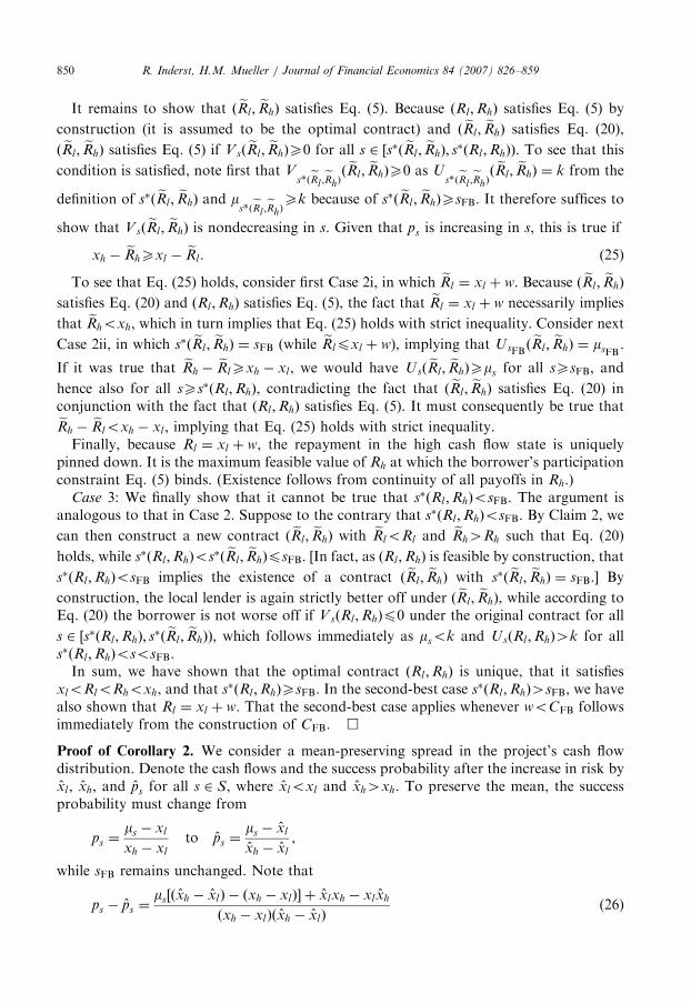
ARTICLE IN PRESSR. Inderst, H.M. Mueller / Journal of Financial Economics 84 (2007) 826–859850
It remains to show that ð eRl ; eRhÞ satisfies Eq. (5). Because ðRl ;RhÞ satisfies Eq. (5) by
construction (it is assumed to be the optimal contract) and ð eRl ; eRhÞ satisfies Eq. (20),
ð eRl ; eRhÞ satisfies Eq. (5) if Vsð eRl ; eRhÞX0 for all s 2 ½s�ð eRl ; eRhÞ; s�ðRl ;RhÞÞ. To see that this
condition is satisfied, note first that Vs�ðeRl ;
eRhÞð eRl ; eRhÞX0 as U
s�ðeRl ;eRhÞð eRl ; eRhÞ ¼ k from the
definition of s�ð eRl ; eRhÞ and ms�ðeRl ;
eRhÞXk because of s�ð eRl ; eRhÞXsFB. It therefore suffices to
show that V sð eRl ; eRhÞ is nondecreasing in s. Given that ps is increasing in s, this is true if
xh � eRhXxl � eRl . (25)
To see that Eq. (25) holds, consider first Case 2i, in which eRl ¼ xl þ w. Because ð eRl ; eRhÞ
satisfies Eq. (20) and ðRl ;RhÞ satisfies Eq. (5), the fact that eRl ¼ xl þ w necessarily implies
that eRhoxh, which in turn implies that Eq. (25) holds with strict inequality. Consider next
Case 2ii, in which s�ð eRl ; eRhÞ ¼ sFB (while eRlpxl þ w), implying that UsFBð eRl ; eRhÞ ¼ msFB
.
If it was true that eRh � eRlXxh � xl , we would have Usð eRl ; eRhÞXms for all sXsFB, and
hence also for all sXs�ðRl ;RhÞ, contradicting the fact that ð eRl ; eRhÞ satisfies Eq. (20) inconjunction with the fact that ðRl ;RhÞ satisfies Eq. (5). It must consequently be true thateRh � eRloxh � xl , implying that Eq. (25) holds with strict inequality.Finally, because Rl ¼ xl þ w, the repayment in the high cash flow state is uniquely
pinned down. It is the maximum feasible value of Rh at which the borrower’s participationconstraint Eq. (5) binds. (Existence follows from continuity of all payoffs in Rh.)
Case 3: We finally show that it cannot be true that s�ðRl ;RhÞosFB. The argument isanalogous to that in Case 2. Suppose to the contrary that s�ðRl ;RhÞosFB. By Claim 2, we
can then construct a new contract ð eRl ; eRhÞ with eRloRl and eRh4Rh such that Eq. (20)
holds, while s�ðRl ;RhÞos�ð eRl ; eRhÞpsFB. [In fact, as ðRl ;RhÞ is feasible by construction, that
s�ðRl ;RhÞosFB implies the existence of a contract ð eRl ; eRhÞ with s�ð eRl ; eRhÞ ¼ sFB.] By
construction, the local lender is again strictly better off under ð eRl ; eRhÞ, while according toEq. (20) the borrower is not worse off if VsðRl ;RhÞp0 under the original contract for all
s 2 ½s�ðRl ;RhÞ; s�ð eRl ; eRhÞÞ, which follows immediately as msok and UsðRl ;RhÞ4k for alls�ðRl ;RhÞososFB.In sum, we have shown that the optimal contract ðRl ;RhÞ is unique, that it satisfies
xloRloRhoxh, and that s�ðRl ;RhÞXsFB. In the second-best case s�ðRl ;RhÞ4sFB, we havealso shown that Rl ¼ xl þ w. That the second-best case applies whenever woCFB followsimmediately from the construction of CFB. &
Proof of Corollary 2. We consider a mean-preserving spread in the project’s cash flowdistribution. Denote the cash flows and the success probability after the increase in risk byxl , xh, and ps for all s 2 S, where xloxl and xh4xh. To preserve the mean, the successprobability must change from
ps ¼ms � xl
xh � xl
to ps ¼ms � xl
xh � xl
,
while sFB remains unchanged. Note that
ps � ps ¼ms½ðxh � xlÞ � ðxh � xlÞ� þ xlxh � xlxh
ðxh � xlÞðxh � xlÞ(26)
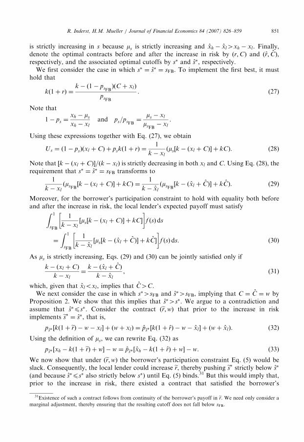
ARTICLE IN PRESSR. Inderst, H.M. Mueller / Journal of Financial Economics 84 (2007) 826–859 851
is strictly increasing in s because ms is strictly increasing and xh � xl4xh � xl . Finally,denote the optimal contracts before and after the increase in risk by ðr;CÞ and ðr; CÞ,respectively, and the associated optimal cutoffs by s� and s�, respectively.
We first consider the case in which s� ¼ s� ¼ sFB. To implement the first best, it musthold that
kð1þ rÞ ¼k � ð1� psFB
ÞðC þ xlÞ
psFB
. (27)
Note that
1� ps ¼xh � ms
xh � xl
and ps=psFB¼
ms � xl
msFB� xl
.
Using these expressions together with Eq. (27), we obtain
Us ¼ ð1� psÞðxl þ CÞ þ pskð1þ rÞ ¼1
k � xl
ðms½k � ðxl þ CÞ� þ kCÞ. (28)
Note that ½k � ðxl þ CÞ�=ðk � xlÞ is strictly decreasing in both xl and C. Using Eq. (28), therequirement that s� ¼ s� ¼ sFB transforms to
1
k � xl
ðmsFB½k � ðxl þ CÞ� þ kCÞ ¼
1
k � xl
ðmsFB½k � ðxl þ CÞ� þ kCÞ. (29)
Moreover, for the borrower’s participation constraint to hold with equality both beforeand after the increase in risk, the local lender’s expected payoff must satisfyZ 1
sFB
1
k � xl
½ms½k � ðxl þ CÞ� þ kC�
� �f ðsÞds
¼
Z 1
sFB
1
k � xl
½ms½k � ðxl þ CÞ� þ kC�
� �f ðsÞds. ð30Þ
As ms is strictly increasing, Eqs. (29) and (30) can be jointly satisfied only if
k � ðxl þ CÞ
k � xl
¼k � ðxl þ CÞ
k � xl
, (31)
which, given that xloxl , implies that C4C.We next consider the case in which s�4sFB and s�4sFB, implying that C ¼ C ¼ w by
Proposition 2. We show that this implies that s�4s�. We argue to a contradiction andassume that s�ps�. Consider the contract ðer;wÞ that prior to the increase in riskimplements es� ¼ s�, that is,
ps� ½kð1þ erÞ � w� xl � þ ðwþ xlÞ ¼ ps� ½kð1þ rÞ � w� xl � þ ðwþ xlÞ. (32)
Using the definition of ms, we can rewrite Eq. (32) as
ps� ½xh � kð1þ erÞ þ w� � w ¼ ps� ½xh � kð1þ rÞ þ w� � w. (33)
We now show that under ðer;wÞ the borrower’s participation constraint Eq. (5) would beslack. Consequently, the local lender could increase er, thereby pushing es� strictly below s�
(and because s�ps� also strictly below s�) until Eq. (5) binds.31 But this would imply that,prior to the increase in risk, there existed a contract that satisfied the borrower’s
31Existence of such a contract follows from continuity of the borrower’s payoff in er. We need only consider a
marginal adjustment, thereby ensuring that the resulting cutoff does not fall below sFB.

ARTICLE IN PRESSR. Inderst, H.M. Mueller / Journal of Financial Economics 84 (2007) 826–859852
participation constraint and implemented a strictly lower cutoff than ðr;wÞ, contradictingthe optimality of ðr;wÞ. The borrower’s participation constraint is slack under ðer;wÞ ifZ 1
s�½psðxh � kð1þ erÞ þ wÞ � w�f ðsÞds
4Z 1
s�½psðxh � kð1þ rÞ þ wÞ � w�f ðsÞds ¼ V , ð34Þ
where the equality follows from the fact that the participation constraint binds under ðr;wÞ.But Eq. (34) is implied by Eq. (33) and the fact that ps � ps is strictly increasing in s.Finally, note that we have from Eq. (8) that CFB4CFB because of xloxl . Hence, the
only remaining case is that in which C ¼ C ¼ w and s�4s� ¼ sFB. &
Proof of Proposition 4. We first prove an auxiliary result.
Claim. Take any contract ðRl ;RhÞ with Rl ¼ xl þ w and Rh4Rl and a different contract
ð eRl ; eRhÞaðRl ;RhÞ satisfying V sð eRl ; eRhÞpV sðRl ;RhÞ for some s ¼ eso1. It holds that
Vsð eRl ; eRhÞoVsðRl ;RhÞ (and therefore that Usð eRl ; eRhÞ4UsðRl ;RhÞÞ for all s4es.Proof. We can rewrite the condition that Vsð eRl ; eRhÞpVsðRl ;RhÞ at s ¼ es as
ð eRl � RlÞ þ ps½ðeRh � eRlÞ � ðRh � RlÞ�X0. (35)
Because Rl ¼ xl þ w, we have that eRl � Rlp0. Hence, for Eq. (35) to hold, it must be true
that eRh � eRlXRh � Rl . There are two cases. If eRl ¼ Rl , then Eq. (35) and eRhaRh together
imply that eRh4Rh, and therefore that ð eRh � eRlÞ � ðRh � RlÞ40. If eRloRl , it follows
directly from Eq. (35) that ð eRh � eRlÞ � ðRh � RlÞ40. Given that ps is strictly increasing in
s, this implies that, in either case,V sð eRl ; eRhÞoV sðRl ;RhÞ for all s4es. &
We can restrict ourselves to the case s�4sFB, which, by Proposition 2, implies that
Rl ¼ xl þ w. Suppose first that the borrower makes a new offer ð eRl ; eRhÞ. For this offer to
be profitable for the borrower, it must hold that s�ð eRl ; eRhÞps�ðRl ;RhÞ. By the definition of
s�ð eRl ; eRhÞ, this implies that k ¼ Us�ðeRl ;
eRhÞð eRl ; eRhÞ4U
s�ðeRl ;eRhÞðRl ;RhÞ and therefore that
Vs�ðeRl ;
eRhÞð eRl ; eRhÞpV
s�ðeRl ;eRhÞðRl ;RhÞ.By Claim 1, it then follows that Vsð eRl ; eRhÞoV sðRl ;RhÞ
and therefore that Usð eRl ; eRhÞ4UsðRl ;RhÞ for all s4s�ð eRl ; eRhÞ. Hence, the local lender
prefers ð eRl ; eRhÞ to ðRl ;RhÞ for all s4s�ð eRl ; eRhÞ, and thus even for values sXs�ðRl ;RhÞ forwhich she would have accepted the borrower under the original contract ðRl ;RhÞ.
Consequently, the local lender’s new expected payoff is Uð eRl ; eRhÞ4UðRl ;RhÞ,while the
borrower’s new expected payoff is V ð eRl ; eRhÞ. As ðRl ;RhÞ maximizes the local lender’s
expected payoff subject to leaving the borrower exactly V , this immediately implies that
the borrower’s expected payoff under ð eRl ; eRhÞ is V ð eRl ; eRhÞoV ðRl ;RhÞ ¼ V , which in turn
implies that offering ð eRl ; eRhÞ cannot be profitable for the borrower. The argument for thecase in which the local lender makes a new offer, which results in a signaling game, isanalogous. &

ARTICLE IN PRESSR. Inderst, H.M. Mueller / Journal of Financial Economics 84 (2007) 826–859 853
Proof of Proposition 5. Before we can prove Proposition 5, we must first verify that somekey results from our base model extend to the setting in Section 5. We first extend theargument from Lemma 2.
Claim 1. For any q40, borrowers who are initially attracted by the local lender but rejected
after the project evaluation cannot obtain financing elsewhere.
Proof. It is now only with probability q40 that the local lender has a more preciseestimate ps of the project’s success probability, while with probability 1� q her estimate isthe same as that of the transaction lenders, namely, p. Moreover, our assumption that onlythe local lender can observe her own success probability estimate implies that only sheknows whether her estimate is more precise.
The expected NPV of a project that has been rejected by the local lender depends,among other things, on the local lender’s decision in case she does not observe s. As can beeasily shown, if the local lender is then indifferent between accepting and rejecting theproject, then, under the optimal contract, she must accept with probability one. To see this,note first that
R 10
UsðRl;RhÞf ðsÞds ¼ k, where substituting UsðRl;RhÞ ¼ ms � V sðRl;RhÞ
yieldsR 10 VsðRl;RhÞf ðsÞds ¼ m� k40. Suppose now that under the optimal contract
ðRl;RhÞ, the local lender randomizes between accepting and rejecting if she is indifferentand does not observe s. But because
R 10 V sðRl;RhÞf ðsÞds40, the borrower’s participation
constraint could be relaxed if the local lender accepted with probability one, implying thatthere exists another contract with a higher repayment that satisfies the borrower’sparticipation constraint with equality while making the local lender strictly better off,contracting the optimality of ðRl;RhÞ.
We first consider the case in which the local lender accepts the borrower if she does notobserve s. We argue to a contradiction and assume that a borrower who is initiallyattracted by the local lender but then rejected can obtain funding from transaction lenders,
that is,R s�
0 ðms � kÞðf ðsÞ=F ðs�ÞÞds40. The borrower’s expected payoff is then
q
Z 1
s�½ms �UsðRl ;RhÞ�f ðsÞdsþ
Z s�
0
ðms � kÞf ðsÞds
" #
þ ð1� qÞ
Z 1
0
½ms �UsðRl ;RhÞ�f ðsÞds. ð36Þ
The requirement that the expression in Eq. (36) be greater than or equal to m� k40transforms to
q
Z 1
s�½k �UsðRl ;RhÞ�f ðsÞdsXð1� qÞ
Z 1
0
½UsðRl ;RhÞ � k�f ðsÞds. (37)
But the fact that the local lender accepts the borrower if she does not observe s implies thatR 10 UsðRl ;RhÞf ðsÞdsXk, which, in conjunction with UsðRl ;RhÞ4k for all s4s�, violates
Eq. (37).We next consider the other case in which the local lender accepts the borrower only if she
observes s and if sXs�. Again, we argue to a contradiction and assume that
ð1� qÞðm� kÞ þ qR s�
0 ðms � kÞf ðsÞds
ð1� qÞ þ qF ðs�Þ40, (38)

ARTICLE IN PRESSR. Inderst, H.M. Mueller / Journal of Financial Economics 84 (2007) 826–859854
that is, we assume that the expected NPV conditional on being rejected by the local lenderis positive, implying that a rejected borrower can obtain funding from transaction lenders.The borrower’s expected payoff is then
q
Z 1
s�½ms �UsðRl ;RhÞ�f ðsÞdsþ ð1� qÞðm� kÞ þ q
Z s�
0
ðms � kÞf ðsÞds. (39)
The requirement that the expression in (39) be greater than or equal to m� k40transforms toZ 1
s�½UsðRl ;RhÞ � k�f ðsÞdso0, (40)
which is again violated as UsðRl ;RhÞ4k for all s4s�. &
Given Claim 1, the borrower’s expected payoff in case the local lender accepts him if shedoes not observe s is
V ðRl ;RhÞ :¼ q
Z 1
s�VsðRl ;RhÞf ðsÞdsþ ð1� qÞ
Z 1
0
V sðRl ;RhÞf ðsÞds, (41)
while the borrower’s expected payoff in case the local lender rejects him if she does notobserve s is
V ðRl ;RhÞ :¼ q
Z 1
s�VsðRl ;RhÞf ðsÞds. (42)
The local lender’s problem is to maximize
UðRl;RhÞ :¼ q
Z 1
s�½UsðRl ;RhÞ � k�f ðsÞds
þ ð1� qÞmax 0;
Z 1
0
½UsðRl ;RhÞ � k�f ðsÞds
� �, ð43Þ
which accounts for the optimality of the local lender’s credit decision, subject to theborrower’s participation constraint V ðRl ;RhÞXV ¼ m� k. By standard arguments, theborrower’s participation constraint must bind at the optimum.We now show that the results from Propositions 1 and 2, which characterize the optimal
contract if the borrower’s participation constraint can be satisfied, straightforwardlyextend to the current setting.
Claim 2. Propositions 1 and 2 extend to the model in Section 5, with the single qualification
that the definition of CFB changes to
CFB ¼ðk � xlÞðm� kÞ
qR 1
sFBðms � kÞf ðsÞdsþ ð1� qÞðm� kÞ
. (44)
Proof. We begin with the definition of CFB. Note first that we can again use the fact that
V sðRl ;RhÞ ¼ CFBms � k
k � xl
, (45)

ARTICLE IN PRESSR. Inderst, H.M. Mueller / Journal of Financial Economics 84 (2007) 826–859 855
which is obtained by substituting s� ¼ sFB and the definition of psFBin Eq. (1). Observe
next that, given that m� k40, we have that psFB4R 10 psf ðsÞds such that UsFB
ðRl ;RhÞ ¼ k
implies thatR 10 UsðRl ;RhÞf ðsÞds4k. In other words, if the first best is attainable, then the
local lender accepts the borrower if she does not observe s. We then obtain Eq. (44) fromthe borrower’s binding participation constraint, where we use V ðRl;RhÞ as defined inEq. (41). Finally, the repayment in the good state, Rh ¼ kð1þ rFBÞ, is still uniquelydetermined by Eq. (9), though we can now substitute CFB from Eq. (44). Accordingly, forall wXCFB, the optimal contract is unique and implements the first-best credit decision.
We next turn to the case in which the first best is not attainable, that is, s�ðRl;RhÞ4sFB.Here, the key argument in the proof of Propositions 1 and 2 was that if the (alleged)optimal contract ðRl;RhÞ does not have the properties asserted in the propositions, then onecan construct a flatter contract ð eRl ; eRhÞ that satisfies the borrower’s participationconstraint while making the local lender strictly better off. Recall from Claim 1 that ifthe lender is indifferent between accepting and rejecting if she does not observe s, thenunder the optimal contract ðRl ;RhÞ, she must accept with probability one. This in turnimplies that if the local lender rejects the borrower under the optimal contract ðRl;RhÞ if shedoes not observe s, then she must strictly prefer to do so. Because all payoffs arecontinuous, the arguments in the proof of Propositions 1 and 2 fully extend to the currentcase. (We only need to multiply all expected payoffs by q.)
We next consider the case in which under ðRl ;RhÞ the local lender accepts the borrower ifshe does not observe s. The arguments from the proof of Propositions 1 and 2 also extendto this case, albeit with some minor modifications. Claim 1 clearly extends, as it onlyconcerns V sð�Þ. We next show that Claim 2 also extends. Given some ðRl ;RhÞ withRloxl þ w, we choose ð eRl ; eRhÞ with eRl4Rl and eRhoRh such that
q
Z 1
s�ðRl ;RhÞ
½Vsð eRl ; eRhÞ � VsðRl ;RhÞ�f ðsÞds
þ ð1� qÞ
Z 1
0
½V ð eRl ; eRhÞ � VsðRl ;RhÞ�f ðsÞds ¼ 0. ð46Þ
In words, if under ð eRl ; eRhÞ the cutoff s� remains unchanged, and if the borrower is accepted
if the local lender does not observe s, then the borrower’s expected payoff under ð eRl ; eRhÞ is
the same as it is under ðRl ;RhÞ. We next show that s�ð eRl ; eRhÞos�ðRl ;RhÞ. Clearly, this istrue if
ps�ðRl ;RhÞ½ðRh � RlÞ � ð eRh � eRlÞ� � ð eRl � RlÞo0, (47)
which, substituting from Eq. (46) and using the fact that eRl � Rl40 and Rh � Rl4eRh � eRl , holds if
ps�ðRl ;RhÞoq
Z 1
s�ðRl ;RhÞ
psf ðsÞdsþ ð1� qÞ
Z 1
0
psf ðsÞds. (48)
Given that UsðRl ;RhÞ is strictly increasing in s and Us�ðRl ;RhÞðRl ;RhÞ ¼ k, the fact thatR 1
0 UsðRl;RhÞf ðsÞdsXk, as the local lender accepts the borrower if she does not observe s,
implies thatR 10 psf ðsÞdsXps�ðRl ;RhÞ
. Together with the fact that ps is strictly increasing, this
yields Eq. (48). It remains to show that under ð eRl ; eRhÞ it is true that the local lender accepts
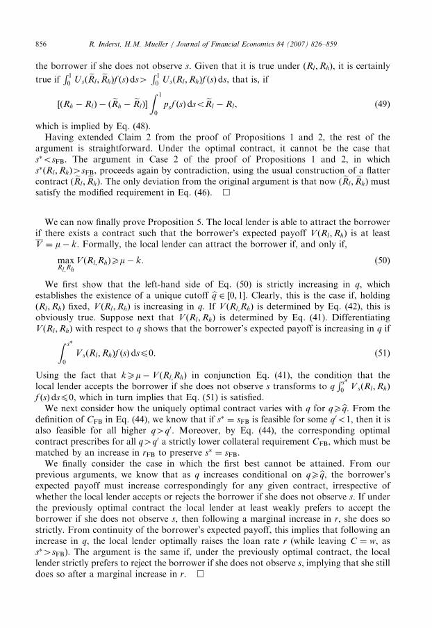
ARTICLE IN PRESSR. Inderst, H.M. Mueller / Journal of Financial Economics 84 (2007) 826–859856
the borrower if she does not observe s. Given that it is true under ðRl ;RhÞ, it is certainly
true ifR 10 Usð eRl ; eRhÞf ðsÞds4
R 10 UsðRl ;RhÞf ðsÞds, that is, if
½ðRh � RlÞ � ð eRh � eRlÞ�
Z 1
0
psf ðsÞdso eRl � Rl , (49)
which is implied by Eq. (48).Having extended Claim 2 from the proof of Propositions 1 and 2, the rest of the
argument is straightforward. Under the optimal contract, it cannot be the case thats�osFB. The argument in Case 2 of the proof of Propositions 1 and 2, in whichs�ðRl ;RhÞ4sFB, proceeds again by contradiction, using the usual construction of a flattercontract ð eRl ; eRhÞ. The only deviation from the original argument is that now ð eRl ; eRhÞ mustsatisfy the modified requirement in Eq. (46). &
We can now finally prove Proposition 5. The local lender is able to attract the borrowerif there exists a contract such that the borrower’s expected payoff V ðRl ;RhÞ is at leastV ¼ m� k. Formally, the local lender can attract the borrower if, and only if,
maxRl;Rh
V ðRl;RhÞXm� k. (50)
We first show that the left-hand side of Eq. (50) is strictly increasing in q, whichestablishes the existence of a unique cutoff bq 2 ½0; 1�. Clearly, this is the case if, holdingðRl ;RhÞ fixed, V ðRl ;RhÞ is increasing in q. If V ðRl;RhÞ is determined by Eq. (42), this isobviously true. Suppose next that V ðRl ;RhÞ is determined by Eq. (41). DifferentiatingV ðRl ;RhÞ with respect to q shows that the borrower’s expected payoff is increasing in q ifZ s�
0
V sðRl ;RhÞf ðsÞdsp0. (51)
Using the fact that kXm� V ðRl;RhÞ in conjunction Eq. (41), the condition that thelocal lender accepts the borrower if she does not observe s transforms to q
R s�
0 V sðRl ;RhÞ
f ðsÞdsp0, which in turn implies that Eq. (51) is satisfied.We next consider how the uniquely optimal contract varies with q for qXbq. From the
definition of CFB in Eq. (44), we know that if s� ¼ sFB is feasible for some q0o1, then it isalso feasible for all higher q4q0. Moreover, by Eq. (44), the corresponding optimalcontract prescribes for all q4q0 a strictly lower collateral requirement CFB, which must bematched by an increase in rFB to preserve s� ¼ sFB.We finally consider the case in which the first best cannot be attained. From our
previous arguments, we know that as q increases conditional on qXbq, the borrower’sexpected payoff must increase correspondingly for any given contract, irrespective ofwhether the local lender accepts or rejects the borrower if she does not observe s. If underthe previously optimal contract the local lender at least weakly prefers to accept theborrower if she does not observe s, then following a marginal increase in r, she does sostrictly. From continuity of the borrower’s expected payoff, this implies that following anincrease in q, the local lender optimally raises the loan rate r (while leaving C ¼ w, ass�4sFB). The argument is the same if, under the previously optimal contract, the locallender strictly prefers to reject the borrower if she does not observe s, implying that she stilldoes so after a marginal increase in r. &
ARTICLE IN PRESSR. Inderst, H.M. Mueller / Journal of Financial Economics 84 (2007) 826–859 857
Proof of Proposition 6. It is straightforward to extend the argument from the proof ofProposition 5 to show that
CFB :¼ðk � xlÞðm� k � kÞ
qR 1
sFBðms � kÞf ðsÞdsþ ð1� qÞðm� kÞ
, (52)
which is strictly decreasing in k.32 Consequently, if the competitive pressure fromtransaction lenders increases (lower k), the optimal collateral requirement increasescorrespondingly. Naturally, rFB must decrease. If the first best cannot be attained,implying that C ¼ w, it follows immediately that r must decrease, which in turn impliesthat s� must increase.
As for the second part of the claim, differentiating Eq. (52) with respect to q and k, while
noting thatR 1
sFBðms � kÞf ðsÞds4m� k from the definition of sFB, yields d
2CFB=dqdk40.
Of course, if the first best is unattainable, we invariantly have that C ¼ w. &
References
Almazan, A., 2002. A model of competition in banking: bank capital vs. expertise. Journal of Financial
Intermediation 11, 87–121.
Avery, R.B., Bostic, R.W., Samolyk, K.A., 1998. The role of personal wealth in small business finance. Journal of
Banking and Finance 22, 1019–1061.
Berger, A.N., Frame, W.S., 2007. Small business scoring and credit availability. Journal of Small Business
Management 45, 5–22.
Berger, A.N., Udell, G.F., 1990. Collateral, loan quality, and bank risk. Journal of Monetary Economics 25,
21–42.
Berger, A.N., Udell, G.F., 1995. Relationship lending and lines of credit in small firms finance. Journal of
Business 68, 351–381.
Berger, A.N., Udell, G.F., 1998. The economics of small business finance: the roles of private equity and debt
markets in the financial growth cycle. Journal of Banking and Finance 22, 613–673.
Berger, A.N., Frame, W.S., Miller, N.M., 2005. Credit scoring and the availability, price, and risk of small
business credit. Journal of Money, Credit, and Banking 37, 191–222.
Bernanke, B.S., Gertler, M., Gilchrist, S., 1999. The financial accelerator in a quantitative business cycle
framework. In: Taylor, J., Woodford, M. (Eds.), Handbook of Macroeconomics, vol. 1, North-Holland,
Amsterdam, pp. 1341–1393 (Chapter 21).
Besanko, D., Thakor, A.V., 1987a. Collateral and rationing: sorting equilibria in monopolistic and competitive
credit markets. International Economic Review 28, 671–689.
Besanko, D., Thakor, A.V., 1987b. Competitive equilibrium in the credit market under asymmetric information.
Journal of Economic Theory 42, 167–182.
Bester, H., 1985. Screening vs. rationing in credit markets with imperfect information. American Economic
Review 75, 850–855.
Boot, A.W.A., 2000. Relationship banking: what do we know? Journal of Financial Intermediation 9, 7–25.
Boot, A.W.A., Thakor, A.V., 1994. Moral hazard and secured lending in an infinitely repeated credit market
game. International Economic Review 35, 899–920.
Boot, A.W.A., Thakor, A.V., 2000. Can relationship banking survive competition? Journal of Finance 55,
679–713.
Boot, A.W.A., Thakor, A.V., Udell, G.F., 1991. Secured lending and default risk: equilibrium analysis, policy
implications and empirical results. Economic Journal 101, 458–472.
32This condition is obtained from inserting V ðRl ;RhÞ ¼ qR 1
s�VsðRl ;RhÞf ðsÞdsþ ð1� qÞ
R 10 VsðRl ;RhÞf ðsÞds
and V sðRl ;RhÞ ¼ CFBðms � kÞ=ðk � xlÞ, where the latter condition follows from s� ¼ sFB, into the binding
participation constraint V ðRl ;RhÞ ¼ m� k � k.

ARTICLE IN PRESSR. Inderst, H.M. Mueller / Journal of Financial Economics 84 (2007) 826–859858
Broecker, T., 1990. Credit-worthiness tests and interbank competition. Econometrica 58, 429–452.
Brunner, A., Krahnen, J.P., Weber, M., 2000. Information production in credit relationships: on the role of
internal ratings in commercial banking. Center for Financial Studies Working Paper 2000/10. University of
Frankfurt, Germany.
Chan, Y.-S., Kanatas, G., 1985. Asymmetric valuations and the role of collateral in loan agreements. Journal of
Money, Credit and Banking 17, 84–95.
Chan, Y.-S., Thakor, A.V., 1987. Collateral and competitive equilibria with moral hazard and private
information. Journal of Finance 42, 345–363.
Cole, R.A., Goldberg, L.G., White, L.J., 2004. Cookie cutter vs. character: the micro structure of small business
lending by large and small banks. Journal of Financial and Quantitative Analysis 39, 227–251.
Degryse, H., van Cayseele, P., 2000. Relationship lending within a bank-based system: evidence from European
small business data. Journal of Financial Intermediation 9, 90–109.
Dennis, S., Nandy, D., Sharpe, I.G., 2000. The determinants of contract terms in bank revolving credit
agreements. Journal of Financial and Quantitative Analysis 35, 87–110.
DeYoung, R., Hunter, W.C., Udell, G.F., 2004. The past, present, and probable future for community banks.
Journal of Financial Services Research 25, 85–133.
Frame, W.S., Srinivasan, A., Woosley, L., 2001. The effect of credit scoring on small-business lending. Journal of
Money, Credit, and Banking 33, 813–825.
Frame, W.S., Padhi, M., Woosley, L., 2004. Credit scoring and the availability of small business credit in low- and
moderate-income areas. Financial Review 39, 35–54.
Guiso, L., Sapienza, P., Zingales, L., 2004. Does informed financial development matter? Quarterly Journal of
Economics 119, 929–969.
Hannan, T.H., 2003. Changes in non-local lending to small business. Journal of Financial Services Research 24,
31–46.
Hauswald, R., Marquez, R., 2003. Information technology and financial services competition. Review of
Financial Studies 16, 921–948.
Hauswald, R., Marquez, R., 2006. Competition and strategic information acquisition in credit markets. Review of
Financial Studies 19, 967–1000.
Inderst, R., Mueller, H.M., 2006. Informed lending and security design. Journal of Finance 61, 2137–2162.
Innes, R., 1990. Limited liability and incentive contracting with ex-ante action choices. Journal of Economic
Theory 52, 45–67.
Jappelli, T., Pagano, M., 2002. Information sharing, lending and defaults: cross-country evidence. Journal of
Banking and Finance 26, 2017–2045.
Jimenez, G., Saurina, J., 2004. Collateral, type of lender and relationship banking as determinants of credit risk.
Journal of Banking and Finance 28, 2191–2212.
Jimenez, G., Salas, V., Saurina, J., 2006a. Determinants of collateral. Journal of Financial Economics 81,
255–281.
Jimenez, G., Salas, V., Saurina, J, 2006b. Collateral in business loans: information asymmetry or cost of
delegation? Unpublished Working Paper. Bank of Spain.
Leeth, J.D., Scott, J.A., 1989. The incidence of secured debt: evidence from the small business community. Journal
of Financial and Quantitative Analysis 24, 379–394.
Manove, M., Padilla, A.J., Pagano, M., 2001. Collateral vs. project screening: a model of lazy banks. Rand
Journal of Economics 32, 726–744.
Mester, L.J., 1997. What’s the point of credit scoring? Federal Reserve Bank of Philadelphia Business Review,
September/October, pp. 3–16.
Petersen, M.A., Rajan, R.G., 1994. The benefits of lending relationships: evidence from small business data.
Journal of Finance 49, 3–37.
Petersen, M.A., Rajan, R.G., 1995. The effect of credit market competition on lending relationships. Quarterly
Journal of Economics 110, 407–443.
Petersen, M.A., Rajan, R.G., 2002. Does distance still matter? The information revolution in small business
lending. Journal of Finance 57, 2533–2570.
Rajan, R.G., 1992. Insiders and outsiders: the choice between informed and arm’s length debt. Journal of Finance
47, 1367–1399.
Rajan, R.G., Winton, A., 1995. Covenants and collateral as incentives to monitor. Journal of Finance 50,
1113–1146.
Reid, G.C., 1991. Staying in business. International Journal of Industrial Organization 9, 545–556.

ARTICLE IN PRESSR. Inderst, H.M. Mueller / Journal of Financial Economics 84 (2007) 826–859 859
Saunders, A., Thomas, H., 2001. Financial Institutions Management, Second Canadian Edition. McGraw-Hill
Ryerson, Toronto, Canada.
Thakor, A.V., 1996. Capital requirements, monetary policy, and aggregate bank lending: theory and empirical
evidence. Journal of Finance 51, 279–324.
Villas-Boas, J.M., Schmidt-Mohr, U., 1999. Oligopoly with asymmetric information: differentiation in credit
markets. Rand Journal of Economics 30, 375–396.
Zuckerman, S., 1996. Taking Small Business Competition Nationwide. U.S. Banker, August, pp. 24–28.