A LARGER PIE THROUGH A FAIR SHARE?

GENDER EQUALITY AND ECONOMIC PERFORMANCE

A Geske Dijkstra

April 2000

Working Paper 315

The Institute of Social Studies is Europe's longest-established centre of higher education andresearch in development studies. Post-graduate teaching programmes range from six-weekdiploma courses to the PhD programme. Research at ISS is fundamental in the sense of laying ascientific basis for the formulation of appropriate development policies. The academic work ofISS is disseminated in the form of books, journal articles, teaching texts, monographs andworking papers. The Working Paper series provides a forum for work in progress which seeksto elicit comments and generate discussion. The series includes the research of staff, PhDparticipants and visiting fellows, and outstanding research papers by graduate students.

For further information contact:ORPAS - Institute of Social Studies - P.O. Box 29776

2502LT The Hague - The Netherlands - FAX: +31 70 4260799E-mail: workingpapers@iss.nl

ISSN 0921-0210

Comments are welcome and should be addressed to the author:

CONTENTS

1.I NTRODUCTION 1

2. GENDER EQUALITY AND ECONOMIC PERFORMANCE 2

2.1 The labour market 3

2.2 Unpaid work 5

2.3 The distribution of income and other assets within the household 6

2.4 Conclusion 7

3. UNDP'S MEASURES OF GENDER EQUALITY 8

3.1 From variable to indicator: methodology 10

3.2 The composite index 13

3.3 Conclusion 14

4. TOWARDS A STANDARDISED INDEX OF GENDER EQUALITY (SIGE) 15

4.1 The choice of indicators 18

4.2 The composite index 21

5. RESULTS AND FURTHER ANALYSIS 22

5.1 Further analysis 24

5.2 Gender equality and economic development 26

6. CONCLUSION 28

ENDNOTES 28

REFERENCES 29

APPENDIX 32

1

ABSTRACT

Is gender equality of influence on economic development? Based on insights

from feminist macroeconomics, the paper develops a framework that suggests that the

gendered distribution of the pie does matter for its size. However, in order to assess the

relationship, we need a good measure of gender equality that is not influenced by abso-

lute levels of development. The often-used composite indices developed by UNDP,

GDI and GEM, suffer from conceptual and methodological weaknesses which are ana-

lysed in this paper. The paper then goes on to develop an alternative composite measure

of gender equality. Finally, some first attempts are made to examine the relationship

with economic development.

1

1. INTRODUCTION

The relationship between gender equality and economic development has often

been a topic for debate. A first question is whether economic development improves the

position of women. Many feminist social scientists are sceptical about this. They argue

that economic development may improve the situation of women in some respects, but

that it brings new inequalities at the same time. For example, an increased labour mar-

ket participation of women is accompanied by new subordination in the working place

and/or by a double burden (see Benería and Feldman 1992). The extensive literature on

the impact of structural adjustment programs on women often concludes on a worsen-

ing position of women (Afshar and Dennis 1992, Sparr 1994). However, these studies

are often based on limited data and weak methodological designs. Data for before ad-

justment are often not available, and even if they are it is difficult to assess the counter-

factual: what would have happened in the absence of adjustment. The concept "femini-

sation of poverty" also implies a worsening of the position of women, but its empirical

justification is often weak.

Other studies take a longer timeframe into account, but they focus on just one

aspect of gender inequality. In both cross-section analysis and in a longitudinal study

for the USA, Goldin (1994) finds a U-shaped relationship between economic develop-

ment and gender equality. However, her definition of "gender equality" is limited to

female labour market participation. Norris (1992) develops a model showing that gen-

der inequality increases over time, but she includes only labour market variables in her

definition of inequality.

A question that has been asked more recently, is whether gender equality leads

to a better macroeconomic performance, as measured, for example, in a higher Gross

Domestic Product (GDP). Is the gender distribution of the pie relevant for its size? Or,

in other words, does it matter who makes the pie and who eats it? The answer of main-

stream economists is that it does not. The total size of the pie is maximised if all re-

sources are used where their productivity is largest. A market economy will automati-

cally provide this maximum. However, this concept of allocative efficiency is based on

a given distribution of resources. This static theory is not very helpful when analysing a

relationship with economic development. The question then is to what extent another

distribution of resources leads to higher output. This paper draws on insights from

feminist macroeconomics, among other theories, to conclude that gender equality does

2

make a difference for growth.

However, the examples mentioned above show that there is a need for a better

empirical indicator of gender equality, which is not only based on labour market par-

ticipation. In order to use it for assessing the relationship with economic performance,

this indicator should measure gender equality as such, and should not include some as-

sessment of absolute levels of development. Another requirement for a new indicator

for gender equality is that it can be used for comparisons over time and across coun-

tries.

This paper aims to develop such a measure of gender equality and to examine

the relationship of this "Standardised Index of Gender Equality" with economic devel-

opment. The next section examines the theoretical basis for assuming that more gender

equality leads to better macroeconomic performance. This analysis also provides clues

for the dimensions that have to be included in a measure of gender equality. We then

continue by examining the two measures developed by UNDP in its Human Develop-

ment Report 1995, the Gender-related Development Index (GDI) and the Gender

Empowerment Measure (GEM), showing why they are not appropriate for our pur-

poses. After this, we develop our own "Standardised Index of Gender Equality" (SIGE),

analyse the results, and relate this index to economic development. The last section

concludes.

2. GENDER EQUALITY AND ECONOMIC PERFORMANCE

The total size of the pie is at its maximum if all resources are used where they

have the highest productivity, or when marginal productivity of all resources is equal.

This leads to maximum for allocative efficiency. The assumptions for this criterion of

“Pareto optimality” - also formulated as no one can be made better off without another

person being made worse-off - include perfect competition and the absence of external-

ities. But this criterion also abstracts from the distribution of assets, and it takes a per-

son's preferences as given.

In fact, the distribution of resources over women and men (assets such as edu-

cation, employment) is determined by institutions, rules, laws and power relations and

by ideas on what is feminine and masculine. This given distribution will then set the

stage for the current allocation of resources, and may hamper women to fully develop

their potential. Preferences may also be less "autonomous" than would appear at first

3

sight (Bruyn-Hundt and Kuiper 1994, Seiz 1992, Woolley 1993). They are influenced

by culture but also by the practical barriers which women, in particular, face to "exit" a

given subordinate position. Several authors have pointed to the inconsistency of as-

sumptions underlying economic theories: individuals behave perfectly rational and seek

self-interest in the market, while behaving completely altruistic in the household (Fer-

ber and Nelson 1993, Folbre 1994). While economists tend to think that individuals

choose, sociologists often stress that there is no choice at all. A realistic social science

will have to recognise that there are elements of “agency” and of “constraint” in all be-

haviour. As Folbre put it, it is important to examine the "structures of constraint" (Fol-

bre 1994). In her view, these structures of constraint follow from assets, rules, norms

and preferences.

The emerging feminist macroeconomics (see Bakker 1994, Cagatay et al. 1995,

Elson 1995) has drawn attention to the existence of gender bias in macroeconomic

analysis. The gender bias not only results in less equal outcomes for men and women,

but may also reduce the effectiveness of macroeconomic policies themselves. This is

because most macroeconomic analysis does not take into account the different positions

of men and women in the economy. For this reason, thinking along gender lines is nec-

essary in order to improve our understanding of macroeconomic phenomena. The dif-

ferent positions of men and women are, in particular, visible at three levels (Elson

1995):

1. The labour market;

2. Unpaid work;

3. The distribution of income and other assets within households.

These levels can be applied to a general analysis of the impact of gender ine-

quality on macroeconomic performance. We examine these levels in turn, in order to

assess whether the size of the pie may be affected by its distribution, and what aspects

of gender inequality are responsible for it.

2.1 The labour market

Women and men occupy different positions in the labour market. There is both

horizontal and vertical sex segregation on the labour market: women and men are in

different occupations. In general, men occupy the higher labour market positions. In

addition, women's wages are lower than men's wages everywhere (they constitute about

4

70%); they are also lower if corrected for education and experience (Bartels and De

Groot 1997). If this difference would be fully due to biological differences, there would

be nothing to worry about for economists. If it is due to other factors, however, it means

that another allocation of men and women over labour market positions would produce

higher output.

Evidence is piling up that other factors are important. First, the gender typing of

occupations is not equal in different cultures and is changing over time. While until re-

cently medical doctor was a male job in the Netherlands, it was a female job in the So-

viet Union and is a mixed job in the Netherlands now (although some medical occupa-

tions are -still- predominantly carried out by men). This shows that cultural factors are

important, as well as opportunities and constraints for women to study and to carry out

this occupation. In some cultures, farming is seen as a male job (Northern India) while

in others, most farming activities are carried out by women (many African countries).

Laws and regulations also inhibit women to participate on the labour market. In Af-

ghanistan women are prohibited to perform a job outside the house, and not so long ago

married women were fired from government service in the Netherlands. In many parts

of the world, women have less access to education. In others, where education levels

are equal, studies show that explicit and implicit rules and norms inhibit women to

break the "glass ceiling" to higher management positions (Moss Kanter 1993). In sum,

the allocation of men and women over different labour market positions is not the result

of different capacities only, but also to other factors. If so, then the allocation is subop-

timal and can be expected to lower macroeconomic outcomes.

It seems to be a combination of culture, rules, access to other assets such as edu-

cation, and power that causes the lower labour market position of women. Thus, this

combination of factors is responsible for a suboptimal allocation of production factors,

in this case, female and male labour. The allocative efficiency of the economy can be

improved if women have equal access to education, and if more jobs are allocated ac-

cording to capabilities and not according to customs, rules or cultural ideas regarding

masculine and feminine jobs. Apart from this one-time improvement in allocative effi-

ciency leading to a once-and-for-all increase in GDP, one can also hypothesise that dy-

namic efficiency of the economy will improve. A permanently higher growth rate could

be the result of the beneficial effect of having "mixed teams" at all levels in labour or-

ganisations (Van Witteloostuin 1994).

5

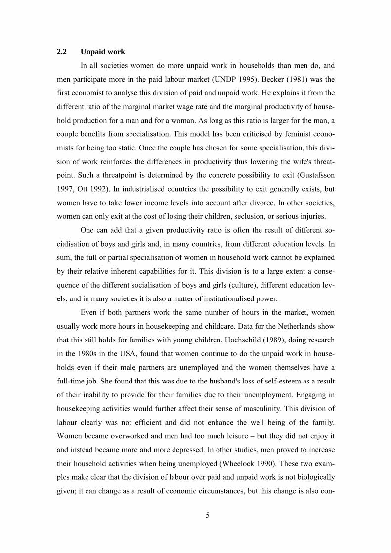
2.2 Unpaid work

In all societies women do more unpaid work in households than men do, and

men participate more in the paid labour market (UNDP 1995). Becker (1981) was the

first economist to analyse this division of paid and unpaid work. He explains it from the

different ratio of the marginal market wage rate and the marginal productivity of house-

hold production for a man and for a woman. As long as this ratio is larger for the man, a

couple benefits from specialisation. This model has been criticised by feminist econo-

mists for being too static. Once the couple has chosen for some specialisation, this divi-

sion of work reinforces the differences in productivity thus lowering the wife's threat-

point. Such a threatpoint is determined by the concrete possibility to exit (Gustafsson

1997, Ott 1992). In industrialised countries the possibility to exit generally exists, but

women have to take lower income levels into account after divorce. In other societies,

women can only exit at the cost of losing their children, seclusion, or serious injuries.

One can add that a given productivity ratio is often the result of different so-

cialisation of boys and girls and, in many countries, from different education levels. In

sum, the full or partial specialisation of women in household work cannot be explained

by their relative inherent capabilities for it. This division is to a large extent a conse-

quence of the different socialisation of boys and girls (culture), different education lev-

els, and in many societies it is also a matter of institutionalised power.

Even if both partners work the same number of hours in the market, women

usually work more hours in housekeeping and childcare. Data for the Netherlands show

that this still holds for families with young children. Hochschild (1989), doing research

in the 1980s in the USA, found that women continue to do the unpaid work in house-

holds even if their male partners are unemployed and the women themselves have a

full-time job. She found that this was due to the husband's loss of self-esteem as a result

of their inability to provide for their families due to their unemployment. Engaging in

housekeeping activities would further affect their sense of masculinity. This division of

labour clearly was not efficient and did not enhance the well being of the family.

Women became overworked and men had too much leisure – but they did not enjoy it

and instead became more and more depressed. In other studies, men proved to increase

their household activities when being unemployed (Wheelock 1990). These two exam-

ples make clear that the division of labour over paid and unpaid work is not biologically

given; it can change as a result of economic circumstances, but this change is also con-

6

tingent upon cultural factors. Allocative efficiency can be improved if the division of

paid and unpaid work is based on relative capabilities. Dynamic efficiency effects can

also be expected, since we can hypothesise that a larger contribution of men to house-

hold and caring activities will improve the quality of these services: children, in par-

ticular, will benefit from having more and better contact with their fathers.

2.3 The distribution of income and other assets within the household

The household is the locus for the distribution of several important assets, such

as food, clothing, love and care, education and access to formal education, informal

health care and access to formal health care, income, leisure and sleep. In economic

theory the household was long taken as a unit, implicitly assuming that there was an

equal distribution within it. More and more evidence is available to show that this is not

the case. The household proves to be a place of violence, discrimination and neglect.

Women and children are particularly vulnerable. For some poor societies it has been

shown that girls are substantially more undernourished than boys (Miller 1981, Sen and

Sengupta 1983). In several countries the sex ratio is negative for women and this can

only be explained from sex-specific abortion and infanticide, and from giving girl-

babies less food and medical services than boy-babies.

In many societies, girls have less access to education and health care than boys

do. Not much is known about the distribution of income within households, but in

many societies (Latin America, Asia) there is evidence that men consume part of their

income for their own consumption and leisure activities, before spending it for basic

necessities of their families. If women have access to earnings, they tend to spend all on

basic necessities for the family. In Africa, the concept of "household income" does not

seem to be relevant at all: women and men have their own income and expenditure re-

sponsibilities within the household (Dwyer and Bruce 1988).

In almost all countries, women work longer hours than men do if both paid and

unpaid work is taken into account (UNDP 1995). In poor societies the difference seems

to be even larger. Poor women with young children reduce sleeping hours to a bare

minimum and do not have any leisure. This means that in almost all countries, men en-

joy more leisure and sleep than women do.

It is unlikely that this division of leisure and sleep is always determined by effi-

ciency motives. Nor does there appear to be an economic reason for giving less food to

7

women and girls. It seems that the distribution of consumption, health and education,

and time, is the result of power relations in the household, but also of norms, rules and

culture. Gains at the macro-level can be expected from a better distribution of assets

within the household between girls and boys, and between women and men. A better

distribution of time for leisure and sleep, and also of food between men and women

will lead to immediate gains in the performance of women. At the macroeconomic

level, these gains will outweigh eventual negative effects on the performance of men,

resulting in a higher GDP. Assuming that there are no differences given by nature in the

“level” of the economic contributions of women and men to society, this net positive

effect comes about. This can be called an allocative efficiency effect. A better distribu-

tion of assets (food, education, etc.) over girls and boys also implies a better allocation

of investment in human capital. This will improve women's market performance in the

future and these gains can be called dynamic efficiency effects.

2.4 Conclusion

From this overview of the three levels at which gender inequalities manifest

themselves in the economy, we can draw two conclusions. First, existing gender ine-

qualities in the labour market, in the division of unpaid work and in the distribution of

assets within the household, have consequences for allocative efficiency of the econ-

omy, and probably also for dynamic efficiency (see Table 1 for an overview). Who

makes the pie, and who eats it does make a difference for the size of the pie. A better

allocation of labour market positions and of unpaid work, and a better distribution of

assets within households will lead to a once and for all increase in GDP, and probably

also to higher growth rates.

Table 1. Gender inequalities reduce economic performanceError! Bookmark

not defined.Allocative efficiency Dynamic efficiency

Labour market Suboptimal allocation of femaleand male labour

Organisation theory: mixedteams better

Unpaid work Suboptimal division of paid andunpaid work

Quality of raising childrenimproves

Distribution withinhouseholds

Suboptimal distribution of leisureand sleep, and other assets overwomen and men

Suboptimal distribution ofassets over girls and boysreduces human capital

8

Secondly, the fact that gender inequalities have economic consequences does

not imply that gender inequality can be equalised with inequality in economic factors

such as access to (economic and other) assets. The above analysis points to power, in-

cluding institutionalised power in laws and regulations, and cultural norms and values,

as important aspects of gender inequality. In order to measure gender equality it is thus

necessary to include these other dimensions such as power and culture as well.

3. UNDP'S MEASURES OF GENDER EQUALITY

In its Human Development Report 1995, UNDP has presented two measures of

gender equality (UNDP 1995): the Gender-related Development Index (GDI) and the

Gender Empowerment Measure (GEM). This pioneering work has been important in

raising attention for gender inequality in international policy debates, as well as in rais-

ing attention among academics for the issue of measuring gender inequality. The index

presented in this paper has also been inspired by these UNDP measures and draws on

the good aspects of it, trying to avoid the problematic aspects. It is therefore important

to state what GDI and GEM are and why they do not serve our purposes.

The most important reason is that both GDI and GEM do not measure gender

inequality as such, but some combination of absolute levels of attainment and relative

female attainments. This limitation of the GDI has been recognised before (Bardhan

and Klasen 1999, Dijkstra and Hanmer 2000, White 1997). As White correctly states,

UNDP (1995) is wrong in drawing comparative conclusions on gender equality on the

basis of the countries' GDI scores. As I will show below, this same criticism also holds

for the GEM. Secondly, questions have been asked about the choice of indicators in

both GDI and GEM (Bardhan and Klasen 1999, Dijkstra and Hanmer 2000, Wieringa

1997b). And thirdly, there are problems with the construction of the indices. Bardhan

and Klasen (1999) have brought these forward, in particular for the GDI. The GEM re-

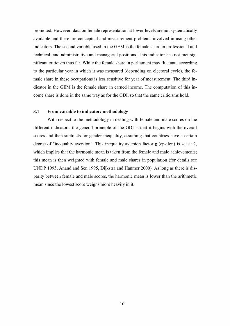
ceived much less attention in this respect. Table 2 summarises the methodologies of

GDI and GEM. In the following, I deal first with the choice of indicators, then with the

limitations of GDI and GEM for measuring gender equality as such and with other

methodological problems involved in indexing and averaging the female and male

scores on the indicators, and finally with problems involved in the construction of the

composite indices.

The GDI uses the same indicators as the earlier introduced Human Development

9

Index (HDI, see UNDP 1990), namely income, life expectancy and education. Income

per capita is here "adjusted" as in the HDI, since it is assumed that above a certain level,

more income does not increase basic human development. With respect to the choice of

variables for the GDI, most criticism has been raised against the income variable (see

Bardhan and Klasen 1999, Dijkstra and Hanmer 2000). This indicator is based on the

female share in the economically active population and on the relative female/male ur-

ban wage rate. Definitions of economically active population vary, however. In par-

ticular, work in family enterprises and in subsistence activities is sometimes included

and sometimes it is not, and this makes a large difference for the outcome. Rural wages

and most informal sector wages are not included, while urban wage rates by sex were

only available for 55 countries. A weighted average of the relative female/male wage

ratio found in these 55 countries (which proved to be 75%) has been used for the other

130 countries. This implies that for most countries, the 75% wage differential is simply

assumed. A final major point of critique against this indicator is that the actual distribu-

tion of income within households is not taken into account. But in practice, it is still

very difficult to include this distribution given the data limitations.

Much less criticisms has been raised against the other two indicators in the GDI,

life expectancy and education, the latter as a combination of literacy rates and combined

primary and secondary enrolment rates. However, a problem with the data on life ex-

pectancy is that they do not include the “missing women”. Comparing the sex ratios for

different countries, it turns out that in some countries, especially in China, Bangladesh,

India and Pakistan, the actual ratio between women and men is much lower than the

expected ratio (Bardhan and Klasen 1999: 990). In these countries, girl babies are often

much less desired than boys, leading to sex-specific abortions or the neglect of female

babies. Although the latter should be reflected in life expectancy ratios, there will often

be deficient reporting of infant mortality. Life expectancy rates will in general not ac-

count for these sex-specific “health risks”.

The GEM is meant to be a measure of female economic and political power.

Critics have pointed to the limited relevance of using the share in parliamentary seats

(Bardhan and Klasen 1999, Wieringa 1997b). In socialist countries this share tends to

be high, but parliaments have only limited power. It has been recommended to look at

female representation in local governance bodies, and to other indicators of female

power such as the strength of women's organisations and the way women's interests are

10

promoted. However, data on female representation at lower levels are not systematically

available and there are conceptual and measurement problems involved in using other

indicators. The second variable used in the GEM is the female share in professional and

technical, and administrative and managerial positions. This indicator has not met sig-

nificant criticism thus far. While the female share in parliament may fluctuate according

to the particular year in which it was measured (depending on electoral cycle), the fe-

male share in these occupations is less sensitive for year of measurement. The third in-

dicator in the GEM is the female share in earned income. The computation of this in-

come share is done in the same way as for the GDI, so that the same criticisms hold.

3.1 From variable to indicator: methodology

With respect to the methodology in dealing with female and male scores on the

different indicators, the general principle of the GDI is that it begins with the overall

scores and then subtracts for gender inequality, assuming that countries have a certain

degree of "inequality aversion". This inequality aversion factor ε (epsilon) is set at 2,

which implies that the harmonic mean is taken from the female and male achievements;

this mean is then weighted with female and male shares in population (for details see

UNDP 1995, Anand and Sen 1995, Dijkstra and Hanmer 2000). As long as there is dis-

parity between female and male scores, the harmonic mean is lower than the arithmetic

mean since the lowest score weighs more heavily in it.

11

Table 2. Methodology for GDI and GEM

Measure Indicators Step 1 (indexation for GDI; penalty forinequality for two GEM indicators)

Step 2 (Penalty for inequality for GDI and oneGEM indicator; indexation for other GEM

indicators)

Overall index

GDI Life expectancy Women live 5 years longer;Index 0-100

Harmonic mean of population-weighted female andmale scores

Adult literacyCombined enrolment,together: education

Index 0-100Index 0-1001/3 enrolment plus 2/3 literacy

Harmonic mean of population-weighted female andmale scores

Simple (arithmetic)average of threescores

Share in adjustedincome, %

Female share in EAP times femalewage/average wage divided by sharein population (= proportional incomeshares)

Harmonic mean of population-weightedproportional income shares;Times adjusted income p.c.;(min=100, max=6,311)

GEM Share in parliament, % Harmonic mean of population-weighted shares

Indexed 0-100 by multiplying by 2

Share in professionaland technical, %; andshare in managementand administrativepositions, %

Harmonic mean of population-weighted share;harmonic mean of population-weighted share

Indexed 0-100 by multiplying by 2;Indexed 0-100 by multiplying by 2;Simple average of the two

Simple (arithmetic)average of threescores

Share in unadjustedincome, %

Female share in EAP times femalewage/average wage (non-agriculturalwages);divided by share in population (=proportional income shares)

Harmonic mean of population-weightedproportional income shares;Times unadjusted income p.c.;Indexed 0-100 (min=100, max=40,000)

12

For income the computation is a bit different. The female (male) share in total

income is divided by share in population to get "proportional income shares" (Table 2).

The harmonic mean of these proportional income shares is then computed. Strangely

enough, in computing this harmonic mean the income shares are again weighted with

shares in population. This is redundant, since shares in earned income have already

been divided by population share. The harmonic mean is then multiplied by adjusted

income per capita. As in the HDI, “adjusted” income means that per capita levels above

average income are discounted.

According to Bardhan and Klasen (1999:993), this means that gender disparities

in income shares have larger consequences at higher income levels than at lower in-

come levels. Although it is technically true that the gender differences are penalised

more at middle income levels than at lower income levels1 this is a consequence of the

fact that the absolute income level weighs heavily in the GDI score. It is very difficult

for poor countries to outperform rich countries on the GDI, no matter how equal they

distribute their income. As long as there is a gender gap, the GDI will be lower than the

HDI. The procedure of multiplying with adjusted income is simply the consequence of

the wish to have a measure that reflects absolute levels of human development as well

as gender inequality. However, this critique from Bardhan and Klasen becomes relevant

if attention is not focused on the GDI itself, but on some measure of difference between

GDI and HDI (as in some of the proposed alternatives, see below). The final step for the

income component is that the outcome is indexed to obtain a value between 0 and 100

(see Table 2).

For the GEM, all three indicators or variables involve female shares in a total

(parliamentary seats, occupations, and income, see Table 2). Theoretically, this could

have led to a simple and direct measure of gender inequality: multiplying the female

share by 2 would give a score on a scale from 0 to 100. However, in order to be "con-

sistent with the methodology applied in the GDI" (UNDP 1995: 132), UNDP opted for

the use of population-weighted harmonic means again, to get "Equally Distributed

Equivalent Percentages" (EDEPs). These EDEPs are then multiplied by 2 to get a score

between 0 and 100. Taking the harmonic mean again means that the GEM is not a di-

rect measure of gender equality either: the harmonic mean of female and male shares is

higher than the female share, and thus softens the inequality. While in the GDI this can

be justified by arguing that absolute levels of well being also matter, there is no such

13

justification for dealing with female share in parliament or in higher occupations.

Another problem is the way income is treated in the GEM. Unlike for the other

variables of the GEM, the population-weighted harmonic mean is not taken from the

shares themselves, but instead from the "proportional income shares" (income share

times share in population) – as in the GDI. Apart from the fact that this again implies

double weighing for population share (as in GDI, see above), this difference in proce-

dures with the other variables of the GEM, is strange. Furthermore, the next step in-

volves multiplying this mean with unadjusted income per capita. UNDP's motivation

for taking unadjusted income is that income in the GEM is valued as a source of power

and not for its contribution to basic development (UNDP 1995: 82). However, as a re-

sult of this multiplying with absolute levels of income per capita, this absolute income

level has a very large impact on the total score of the GEM. The GEM has become an

odd combination of, on the one hand, two variables where relative female power is

counted – albeit softened by their harmonic means, and on the other, one variable in

which the absolute income level per capita weighs heavily. Thus far, these problematic

issues of the GEM have been neglected in the discussion.

An additional problem is that the methodology used for both GDI and GEM of

taking the harmonic mean of the two scores, punishes for inequality no matter whether

female scores are lower or higher than male scores. As a result, a country where

women do better with respect to longevity and education has a lower score (all other

things being equal) than a country where women and men have equal scores for these

two variables. This happens to be the case of Norway, the country used as example in

the 1997 Human Development Report to explain the methodology for the GDI. In other

words, countries where women do better than men on some indicators cannot compen-

sate for other inequalities but are additionally punished.

3.2 The composite index

The third type of weakness of GDI and GEM lies in the construction of the final

indices. In both GDI and GEM a simple arithmetic average is taken of the scores for the

three indicators. It is argued that there are no reasons for the weights of the variables to

be different. However, the variances of the three indicators differ widely and this im-

plies that the indicator with the largest variance has the strongest weight in the overall

index (Harvey et al. 1990, Perrons 1995, Sugarman and Strauss 1988). For the GDI, the

14

income variable has a much larger spread than the other two variables. Bardhan and

Klasen (1999) computed the implied penalties for inequality for the three indicators of

the GDI, showing that the gap in income accounts for 85% of the total gender gap, on

average. This problem - that the overall index is dominated by one of the three compo-

nents - is less severe for the GEM, since the variances of the three components do not

differ as much as in the GDI.

3.3 Conclusion

In sum, the main criticism to GDI and GEM is that they do not measure gender

inequality as such. They combine measures of absolute well being or income with some

measure of inequality. Therefore, neither GDI nor GEM can be used to analyse the re-

lationship between gender equality and economic performance. In addition, there are

other problems with the way GDI and GEM are constructed, with the choice of indica-

tors and the way these indicators are dealt with before they enter as components in the

overall index. In developing an alternative index for gender equality, not so much can

be improved in the choice of indicators since data availability is limited. However, it

can be attempted to avoid the methodological problems.

Several alternative indices have been developed so far, in particular for the GDI.

White's GEQ (Gender Equality index) is defined as the ratio of GDI and HDI (White

1997). Forsythe et al. (1998) focus on gender inequality (GI) which they define as

(HDI-GDI)/HDI. These indices are similar and do measure equality, respectively ine-

quality (see also Anand and Sen 1995, UNDP 1995: 126, 129). However, they still suf-

fer from the other limitations of the GDI, in particular, the peculiar way the income

variable is defined and measured, and the fact that the variation in the overall index is

dominated by the variation in relative income share. Dijkstra and Hanmer (2000) devel-

oped a relative gender equality index (Relative Status of Women, RSW) by taking the

same variables as the GDI but using relative achievements in the three areas. Although

this is a more direct measure than the GEQ or the GI, the other criticisms still hold.

Former socialist countries do well on this index since female labour market participa-

tion is high and this variable dominates the overall index. GEQ, GI and RSW only in-

clude variables related to human development, and exclude the power dimension that is

measured in the GEM.

Bardhan and Klasen (1999) have computed a revised GDI. Their GDI attempts

15

to solve the de facto unequal weighting of the three components, in two ways: First,

they limited the maxima and minima against which actual achievements in life expec-

tancy and education are related to actual minima and maxima over all observations,

thus broadening the range of possible achievements. Secondly, they used different “ine-

quality aversion” factors epsilon for the different components, with the lowest epsilon

for the income component and the highest for life expectancy (respectively 1.5, 3 and

6). Although this is an improvement of the GDI, this measure still compounds absolute

levels of human development with relative female-male achievements.2

Apodaca (1998) develops an index composed of seven indicators that measure

women’s relative economic and social rights. However, some of the indicators she uses

are problematic, and she does not solve the problem of the implicit unequal weights.

This is what we will do now.

4. TOWARDS A STANDARDISED INDEX OF GENDER EQUALITY

(SIGE)

Ideally, a new measure of gender equality should meet the following require-

ments:

1. It should be a relative measure, that is, it should measure gender (in)equality and not

some combination of absolute well-being and inequality;

2. Data should be available for many countries, should be internationally comparable

and as reliable as possible;

3. The index should comprise of a number of indicators that, taken together, represent all

relevant dimensions of gender equality;

4. The construction of the overall index should be such that there is no unintended

weighing of some factors more heavily than other factors.

It is not possible to satisfy all requirements to the same extent. The requirement

that indicators should measure gender (in) equality implies that indicators for absolute

well being of women, such as maternal mortality rates, are excluded. Only indicators

for which we have gendered statistics qualify for the index.

Data availability is an important constraint, and even if data are available, they

are not always reliable. The database we use is the Women's Statistics Database

(WISTAT) as developed by the UN and available on CD-ROM. The sources for these

data include internationally available statistics such as the International Demographic

16

and Health Surveys and the Yearbooks of International Labour Market Statistics of the

ILO. For some data, WISTAT used national surveys, if available. I used the data from

the 1994 series, which was the latest series available in WISTAT, but in practice data

were often from (around) 1990. This means the information is not very recent. For ex-

ample, data for former socialist countries reflects the situation of these countries when

they were still subject to central planning. Our index can only be considered an illustra-

tion of what is possible on the basis of available statistics. It should not give rise to

conclusions on the current state of gender equality in the different countries.

Furthermore, our knowledge of what the relevant dimensions of gender equality

are, and how these dimensions can be measured, is limited. This holds, in particular, for

measuring gender equality in international perspective.

Possible dimensions of gender equality that can be used in cross-country com-

parisons were discussed in a Workshop held at the Institute of Social Studies in The

Hague, in which researchers from Bhutan, Benin, Costa Rica and the Netherlands par-

ticipated.3 The aim was to define important aspects of gender equality and inequality

that may hold in different cultures. The following eight dimensions were identified

(Wieringa 1997a):

1. Gender identity, which includes cultural issues such as the socialisation of girls

and boys, the rigidity of the sexual division of labour;

2. Autonomy of the body, which refers to the absence of gender-based violence,

control over sexuality, and control over reproduction;

3. Autonomy within the household. This encompasses the freedom to marry and

divorce, right to custody in case of divorce, and decision-making power and ac-

cess to assets within the household;

4. Political power, which includes decision-making at above-household levels such

as municipalities, unions, government, and parliament;

5. Social resources, which refers to the access to health and education

6. Material resources, which refers to access to land, houses, and credit

7. Employment and income; this dimension is about the distribution of paid and

unpaid work, wage differentials, formal and informal labour;

8. Time; this is a separate indicator, and includes the relative access to leisure and

sleep.

There is some overlap between these dimensions and the factors mentioned in

17

the brief theoretical and empirical discussion above. Section 2 concluded that access to

assets is important, as well as power and culture. With respect to access to assets, a dis-

tinction can be made between social and economic assets. These four factors (culture,

power, and social and economic assets) are loosely related to the eight dimensions as

defined in the Workshop. Culture is most closely related to gender identity, but is also

of influence on all other dimensions. Power is also a factor that plays a role in all eight

dimensions, but it is most explicitly related to dimension 4. Dimension 5 of the Work-

shop is social resources and dimensions 6 and 7 deal with access to economic re-

sources. Time, in so far as it is access to leisure and sleep, is a social resource, but it is

also an economic resource.

Unfortunately, it is not possible to use internationally available data for all di-

mensions as identified in the Workshop. It is particularly difficult to find data for gen-

der identity, or more generally, for the cultural factor. However, we can expect cultural

factors to be of influence on many gendered statistics that are available. For example,

women’s culture will be of influence on women’s access to education, as well as on

their relative position the labour market and in parliaments. For autonomy of the body

no internationally available statistics are available either. Another dimension, for which

no data are available yet on a sufficient scale, is time use. In OECD countries, time use

data is generally registered. UNDP (1995) published data for gendered time use for

eight former socialist countries and nine developing countries, but in total this gives

data only for 31 countries.

It is important to include several different aspects or dimensions of gender

equality in our index. All participants in the discussion considered the above-mentioned

eight dimensions important, but it was clear that some of them were more important in

some countries than in others. In some countries, for example, there is no difference in

access to education for boys and girls, while women and men still hold unequal posi-

tions in the labour market. Similarly, in some countries women have access to the la-

bour market but at the cost of having much less time for leisure and sleep, or vice versa:

women have more leisure than men but do not earn their own incomes. This shows that

the different dimensions of gender equality may move together, but not necessarily so.

This fact constitutes a constraint for the construction of an Index, or scale. We

cannot construct it on an empirical basis by looking at internal consistency of the scale.

When an index is constructed of labour market inequality, for example, the different

18

indicators are expected to have a high correlation with each other (see Sugarman and

Straus 1988). The Cronbach alpha can be computed, and those indicators with a too low

correlation with the other indicators and with the overall index are removed from the

index. In our case, however, we cannot conclude from the presence or absence of a re-

lationship with other indicators, on the validity of inclusion of the indicator in the over-

all index.

4.1 The choice of indicators

In the following, I examine a set of variables for which data are readily avail-

able, analysing what dimension of gender equality they represent and how well they

represent it. These variables are given an operational definition by assigning indicators

to them. The choice closely follows the indicators used by UNDP for constructing GDI

and GEM, albeit that the way they enter the index is different. The following five vari-

ables are examined:

1. Relative female/male access to education

2. Relative female/male longevity (life expectancy)

3. Relative female/male labour market participation

4. Female share in administrative and management positions

5. Female share in parliament.

1. Access to education. Relative access to education is perhaps the most impor-

tant and most universal indicator for gender equality. It is one of the components of di-

mension 5, access to social resources. But there is also a relationship with access to

economic resources: the higher the education levels, the more chances women have to

improve employment status and income. Furthermore, higher relative education can be

expected to also increase women’s autonomy in the household and women’s power at

above household levels. Finally, a relation with culture can be assumed: if women and

girls have more access to education this reflects cultural changes in society, and it will

in turn allow more cultural changes in favour of women to come about.

We use figures on the relative female/male ratio of combined primary and sec-

ondary school enrolment and of literacy rates, giving literacy a weight of 2/3 and com-

bined enrolment of 1/3, just as UNDP has done for the GDI (UNDP, 1995). Although

this indicator is relatively undisputed, some criticism can be raised, in particular to the

19

use of school enrolment ratios. These ratios say relatively little on school attendance

and performance. In addition, school enrolment may be high if there is a lot of repeti-

tion: if many relatively old children are enrolled, enrolment rates are raised artificially

since the denominator is based on a certain age cohort. However, since enrolment rates

only constitute 1/3 of this indicator, this problem is not considered to be very serious.

2. Relative access to health. The relative health situation of women can be cap-

tured by relative figures on female/male life expectancy. This indicator reflects eventual

discrimination in access to health services (dimension 5), and through this, it may re-

flect cultural ideas on women and men. But it also measures to some extent women’s

relative access to leisure and sleep, since more sleep and more leisure will generally

foster a longer and healthier life. Since no direct data on access to leisure and sleep

(dimension 8) are available for a sufficient number of countries, this is an advantage.

UNDP (1995) also uses relative life expectancy figures in the GDI, but corrects

them for the fact that women live, on average, five years longer than men. Since our

data are transformed and standardised before they enter the overall index (see below),

we do not need to apply any correction: the higher the relative female/male life expec-

tancy is, the better the relative health situation of women is.

3. Relative female/male labour market participation. This can be measured by

the ratio of the female economic activity rate and the male economic activity rate. Par-

ticipation in the labour market is generally considered a sign of female emancipation. It

usually provides women with an independent income, and many jobs give women ac-

cess to some power. Labour market participation is also assumed to foster women’s

relative autonomy in the household. However, these positive consequences depend on

the kind of integration in the labour market.

Unfortunately, the definitions on "economically active population" vary by

country and sometimes by region within countries. In some countries/regions, unpaid

family labour and work in the subsistence economy are included, in others they are not.

For example, the relative female/male labour market participation is 18 in Mali and 56

in Togo – both West African countries between which we do not expect relative female

labour market participation to differ very much. The large difference must therefore be

due to different operational definitions. Bardhan and Klasen (1999) report large differ-

ences even between Indian states. Obviously, unpaid family labour does not give

women an independent income, nor does it lead to more autonomy in the household.

20

Another problem with this indicator is that a high relative female labour market partici-

pation may imply a double burden for women. If women’s household and caring tasks

are not shared with men, the positive effect of labour market participation is offset by a

negative effect on women’s access to leisure and sleep, and so on women’s well-being

and health. For our index, however, this is not so much a problem as long as we include

the indicator for relative health.

The income dimension is only captured to a limited extent by this indicator. We

could have multiplied this ratio by relative female/male wages, as UNDP does for the

GDI, but for most countries these data are not available. Taking an average of 75% for

all these countries, as UNDP does, is not useful in our context since values will be

standardised later on (see below), and multiplying all values by a constant does not

change standardised outcomes.

4. Female share in technical and professional and in administrative and man-

agement positions. This indicator is used by UNDP as part of the GEM. It is a measure

of access to economic assets, since these jobs are relatively better paid than many other

jobs. Access to administrative and management positions reflects to some extent deci-

sion making power in society, while access to technical and professional occupations

reflects opportunities for career development (UNDP 1995). At the same time, this in-

dicator is also an approximation relative female participation in the formal labour mar-

ket (as opposed to labour market participation in general which may be in unpaid family

labour), albeit that not all sectors are represented.

This indicator is much less sensitive to statistical conventions than the former

on relative labour market participation. It also says something on relative female power.

The higher the share of women in these positions, the more power women have in soci-

ety relative to men. Women in these formal labour market positions will also have more

power and autonomy in the household. In addition, this indicator reflects aspects of

culture. And in comparison to the female share in parliament (see below), it is much

less sensitive to the particular year in which it is registered.

5. Female share in parliament. This is an obvious indicator for relative female

power in society. However, the limitations of this indicator are well-known and have

been pointed out above: it only includes female power at national level, in some coun-

tries parliaments have little power, it is only about formal power, and the figure is sen-

sitive to the particular year in which it is measured. Nevertheless, it seems to be an im-

21

portant indicator for relative female power. One can assume that there is also a relation-

ship between this indicator and cultural factors, as well as with autonomy in the house-

hold. Women cannot be members of parliament if they are not allowed to “go out” by

their husbands or fathers. The main advantage of this indicator is that data are available

for many countries.

4.2 The composite index

For the decision on which of these five indicators to include in the composite

index, we cannot rely on an empirical analysis (see above). From the analysis above, it

seems a good choice to include all five indicators: there are two variables for access to

social assets, two variables for the labour market, and one for relative power in society.

Although all have their weaknesses, the combination of the five and giving them equal

weight can be expected to minimise distortions.

In order to combine these indicators in one index, some elaboration of the raw

data is necessary. All five are relative indicators: female achievements divided by male

achievements, or female shares. In order to avoid the unintended overweighing of one

indicator above others, it is necessary to standardise the raw data. For the construction

of the overall index, we have standardised the initial scores, so we expressed them as

number of standard deviations from the mean of the series, as follows:

zij = (xij - µj) / σj

Where:

xij = score of country i on indicator j, j = 1..5

µj = arithmetic mean of scores of all countries on indicator j

σj = standard deviation of scores of all countries on indicator j

However, mean and standard deviation cannot be meaningfully used if the dis-

tribution is not approximately normal. For this reason, some series had to be trans-

formed.4 The standardisation has been applied to the transformed scores. Finally, a

Standardised Index of Gender Equality (SIGE) was computed by taking a simple arith-

metic mean of the standardised and sometimes first transformed, scores on the indica-

tors. The index Zi for each country i is therefore:

22

See Table 3 for overview of computation of this score. The disadvantage of this

overall index is that the score does not have an intuitive meaning. Figures run from

small negative to small positive numbers, with an average close to zero.

Table 3. Standardised Index of Gender Equality (SIGE)Variable Indicator

1. Relative access to education 2/3 relative literacy rates, 1/3 relativecombined enrolment rate;Simple weighted average of the two

2. Relative access to health Female life expectancy /male lifeexpectancy

3. Relative labour market participation Female activity rate/male activity rate

4. Female share in technical andprofessional, and in administrative andmanagement positions

Sum of numbers of women in theseoccupations/total number of persons inthese occupations

5. Female share in parliament Number of female members/ total membersof parliament

5. RESULTS AND FURTHER ANALYSIS

The Appendix Table shows the results of we combine these five indicators in

one index, the Standardised Index for Gender Equality (SIGE). The index could be

computed for 115 countries. Finland comes on top, followed by Sweden and Denmark.

The Table also shows the original scores for each of the five indicators, and the rank of

each country in each indicator (in italic).

Finland has high ranks for all five indicators, and scores best n female repre-

sentation in parliament. Sweden owes its high score to the high female share in profes-

sional, technical, administrative and management positions (STPAM), but also scores

well on parliamentary representation (SPAR). Apart from several other industrialised

countries (Norway, Canada, Austria), some former socialist countries also do well on

this Index (Poland, Hungary, Bulgaria). The Appendix Table shows that this is not so

much due to their score on female share in parliament, as would be expected, but more

∑=

=n

jiji zZ

15/}{

23

to the high scores on the two labour market variables: relative female labour market

participation (REAP) and STPAM. Poland also has a high score on relative life expec-

tancy for women (RLEXP).

Some Caribbean countries can also be found relatively high: Jamaica (7), Bar-

bados (11), Guyana (12), Suriname (20), Cuba (21), and Trinidad and Tobago. These

countries score well on labour market participation, with the exception of Guyana,

which owes its relatively high score to high female parliamentary representation. Nica-

ragua is the highest Latin American country (at 15), probably due to the socialist poli-

cies in the 1980s that improved women’s relative access to social resources. El Salva-

dor is in the 25th position. In the ranks between 34 and 82 we find all other Latin

American and Caribbean countries. The Philippines is the Asian country with the high-

est rank (24), followed by Thailand (30) and China (43). Most Asian countries are in

much lower ranks, however. Predominantly Muslim countries Bangladesh, Afghanistan

and Pakistan close the list. The highest African country is the relatively rich Botswana

(at 33), and Swaziland (37) and Lesotho (38) follow this country. Rwanda is also just

within the first 50, due to its high rank (1st) on relative female labour market participa-

tion (REAP). Most Sub-Saharan African countries can be found between ranks 50 and

100, however, while most North African countries can be found between 103 and 112.

Surprisingly, the empirical results for the much criticised indicator female share

in parliament do not seem to deviate much from what one would expect a priori. In all

countries the share of women in parliament is low, but it is relatively higher in western

countries where one would expect values that accept women in higher positions to have

changed most. Finland scores highest, while Norway, Sweden, Denmark and the Neth-

erlands are in places 3-6. One exception to this rule is Guyana that ranks 2d on this

variable. The “former socialist country effect” does seem to hold, however, for Cuba

(7th) and China (9th).

El Salvador has the highest score for relative life expectancy (RLEXP), while

Nicaragua ranks 4th on this indicator. These high scores are probably due to the civil

wars that these countries had just gone through. Some former socialist countries (Po-

land, Hungary) also do well on this indicator. The relatively low life expectancy for

men in these countries can probably be explained by high alcohol abuse among men. In

the US, the high score may be due to criminality, which has more victims among men.

With respect to relative female labour market participation (REAP), Rwanda

24

comes in first place, followed by Mozambique and Benin. It is clear that statistical con-

ventions in these countries allow for including women who work as unpaid family

members in subsistence agriculture in the registered labour force. In other countries,

like Guatemala or the earlier mentioned Mali, this is probably not the case. Although

this obviously distorts the results, the inclusion of the other labour market variable

STPAM corrects the distortion to some extent.

5.1 Further analysis

When trying to combine a smaller number of indicators in one Index, the distor-

tions caused by disadvantages of particular indicators come to the fore more sharply.

For example, a subset of three indicators that includes life expectancy brings El Salva-

dor to a much higher position. Subsets that include two labour market variables in ad-

dition to education give higher results for the former socialist countries. An Index com-

bining REDUC, STPAM and SPAR gives a similar rank as SIGE5.

In order to examine the relationships between these indicators, I used the trans-

formed data (where applicable) for the five variables. Table 4 presents the correlation

coefficients between these (transformed) five indicators. Relative access to education

(REDUC) proves to have rather high and statistically significant correlations with rela-

tive life expectancy (RLEXP), female share in parliament (SPAR) and, above all, with

female share in technical and professional, and administrative and management posi-

tions (STPAM). Surprisingly, the correlation between REDUC and REAP proves to be

almost zero and is statistically insignificant.

The relative female/male activity rate (REAP) proves to have a rather low

(22%) but significant correlation with STPAM. The relationship between relative life

expectancy and the two labour market indicators is positive and significant, but not very

high. It is higher for STPAM than for REAP. This does not rule out the possibility of a

trade-off between a higher work burden as reflected in participation in the labour mar-

ket and women’s relative health, but it seems that relative labour market participation

and relative health also move together. They appear to be related more if we deal with

participation in white-collar jobs than for jobs in general. The female share in parlia-

ment has a positive and significant correlation (ranging between 32 and 46%) with all

other indicators.

25

Table 4.Linear bivariate correlation coefficients between SIGE5 and components, in percent

REDUC RLEXP REAP STPAM SPAR SIGE5REDUC 52** 2 73** 43** 78**RLEXP 52** 34** 40** 34** 71**REAP 2** 34** 22** 46** 51**STPAMTable

73** 40** 22** 38** 81**

SPAR 43** 34** 46** 38** 69**SIGE5 78** 71** 51** 81** 69**

** Correlation is significant at 0.01 level.

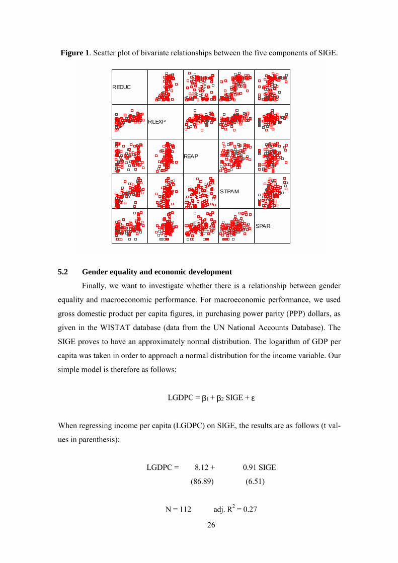
As could be expected, the correlation between the overall index SIGE5 and its

components is high and significant. It is highest for STPAM and REDUC, and lowest

for REAP. The presence or absence of linear relationships between the components is

also confirmed in figure 1, which shows bivariate scatter plots. By looking at the plots,

non-linear relationships can be discerned. The plot for REAP with REDUC confirms

the heterogeneous nature of data on relative economic activity rate: in many countries, a

high score means that women are highly represented in the agricultural subsistence

sector or as unpaid family workers, with low education; in other countries, it points to a

high participation in the formal labour market and it is accompanied by high relative

education. The relationship has the form of a “U”. There is high relative labour market

participation at low relative education levels, and at high relative educational levels,

while it is low at middle educational levels.

Goldin (1994) found a U-shaped relationship between economic development,

measured as GDP per capita, and a related indicator, namely (absolute) female labour

market participation, and she explains it as follows. At low levels of development fe-

male labour market participation is high but is concentrated in agricultural activities.

When education begins to become available, boys benefit first. General income levels

increase but female labour market participation decreases both because of the (family)

income effect and because of a "stigma" (taboo) on married women's outside work. At

higher levels of income, girls also get access to education. In addition, the service sector

expands. The stigma is weaker for the service sector than for manufacturing. These two

factors explain the right side of the "U".

26

Figure 1. Scatter plot of bivariate relationships between the five components of SIGE.

5.2 Gender equality and economic development

Finally, we want to investigate whether there is a relationship between gender

equality and macroeconomic performance. For macroeconomic performance, we used

gross domestic product per capita figures, in purchasing power parity (PPP) dollars, as

given in the WISTAT database (data from the UN National Accounts Database). The

SIGE proves to have an approximately normal distribution. The logarithm of GDP per

capita was taken in order to approach a normal distribution for the income variable. Our

simple model is therefore as follows:

LGDPC = β1 + β2 SIGE + ε

When regressing income per capita (LGDPC) on SIGE, the results are as follows (t val-

ues in parenthesis):

LGDPC = 8.12 + 0.91 SIGE

(86.89) (6.51)

N = 112 adj. R2 = 0.27

REDUC

RLEXP

REAP

STPAM

SPAR

27

This gives a positive and highly significant slope coefficient of .91. This means

that a one full point increase in SIGE is accompanied by 91% growth in income per

capita. The relationship proves to be approximately linear (figure 2). Although these

results confirm the theoretical section of this paper, no definite conclusions can be

drawn on causality. It may also be the case that a higher level of income per capita leads

to more gender equality. Furthermore, it cannot be stated that GDP p.c. is only influ-

enced by gender equality. Many more variables should probably be included in the

model.

Figure 2. Scatter plot of logged GDP per capita (LGDPC) against SIGE.

Nicaragua (135) is a clear outlier (residual is more than three times the standard

deviation), with a much lower GDP per capita than expected according to its level of

gender equality. The relatively high gender equality of Nicaragua can be explained by

public policies carried out under the Sandinista government in the 1980s and probably

also by the strength of the women's movement in that country.5 Zaire (210) also has a

relatively low GDP per capita as compared to its gender equality. On the other side we

find the United Arab Emirates (194) with relatively high GDP and low gender equality.

SIGE5

2.01.51.0.50.0-.5-1.0-1.5-2.0

LGD

PC

11

10

9

8

7

6

5

210

194

135

28

6. CONCLUSION

The paper has examined the relationship between economic development and

gender equality. It showed that there are good theoretical reasons to assume that more

gender equality leads to higher levels of development. The current allocation of labour

market positions over men and women, the distribution of paid and unpaid work, and

the distribution of assets within households, is not based on economic efficiency mo-

tives. I also showed that the measures of gender inequality developed so far (GDI and

GEM, see UNDP 1995) are not suitable for examining this relationship. The main

problem is that absolute levels of development weigh heavily in both these measures.

There are also methodological problems with the construction of the composite indices.

The second part of the paper develops a measure of gender equality that at-

tempts to encompass many possible dimensions of gender equality and that avoids the

conceptual and methodological problems. Obviously, this "Standardised Index of Gen-

der Equality" (SIGE) is not the ultimate measure of gender equality. More data are nec-

essary, in particular, on time use. Another limitation is that most data are for around

1990, which is already dated. However, SIGE can serve as a first approximation of such

an overall index, and it has been constructed according to a much better methodology

than earlier internationally comparable indices.

There proves to be a very strong and significant positive relationship between

this measure of gender equality and economic development. This confirms the expecta-

tions of the theoretical section of the paper. Causality, however, may also run the other

way: gender equality may increase at higher levels of economic development.

ENDNOTES

1. Not between middle and high income levels, since high incomes are adjusted.2 They propose two further alternatives; one solves the problem of the unequal punishing of inequality atdifferent GDP per capita, and the other excludes the problematic income component alltogether. However,the alternatives are still no measure of gender inequality as such.3. See Wieringa (1997a). The Workshop, financed by the Directorate General for International Cooperation(DGIS) of the Dutch Ministry of Foreign Affairs, was the first step of a research project that aims at assess-ing the GDI and GEM indicators for these four countries. The country choice is related to the Agreements onSustainable Development that the Dutch government has concluded with Benin, Bhutan and Costa Rica.4. Given the longer working hours of women in almost all societies, it appears to make more economicsense to provide women with more food and more health services.

5. These policies favoured women's access to primary health care and education, and led to improvements inthe legal status of women (Dijkstra 1998). The low level of GDP is mainly due to prolonged civil war and toeconomic policy failures (Dijkstra 1999).

29

REFERENCES

Afshar, Haleh, and Carolyne Dennis, eds. (1992). Women and Adjustment Policies in the

Third World. London: Macmillan.

Anand, Sudhir, and Amartya Sen (1995). "Gender inequality and human development:

Theories and measurement," Background Papers for Human Development Report

1995. Mimeo (New York, UN Human Development Report Office, August 1995).

Bakker, Isabella (1994). The Strategic Silence: Gender and Economic Policy. London:

Zed Books.

Bartels, C.P.A, and T. de Groot, "Economische prestaties van mannen en vrouwen,"

Economisch Statistische Berichten, Vol. 81, No. 4075 (2 October 1996), pp. 808-812.

Bardhan, Kalpana and Stephan Klasen (1999). "UNDP's gender-related indices: A critical

review", World Development Vol. 27, No. 6 (June), pp. 985-1010.

Becker, Gary (1981). A Treatise on the Family. Boston: Harvard University Press.

Benería, Lourdes, and Shelley Feldman, eds. (1992). Unequal Burden: Economic Crisis,

Persistent Poverty, and Women's Work. Boulder, Co: Westview Press, pp. 239-258.

Bruyn-Hundt, M. (1996). The Economics of Unpaid Work. Amsterdam: Thesis

Publishers.

Bruyn-Hundt, Marga and Edith Kuiper (1994). "De vrouw achter de homo economicus",

Tijdschrift voor Politieke Ekonomie 17, No. 2, September, pp. 48-62.

Cagatay, Nilufer, Diane Elson and Caren Grown (1995), editors of "Gender, Adjustment

and Macroeconomics", special issue of World Development Vol. 23, No. 11.

Dijkstra, A. Geske (1998). "Crisis, adjustment and the dynamics of gender relations in

Central America and the Caribbean". Working Paper No. 277, Institute of Social

Studies, The Hague.

Dijkstra, A. Geske (1999). “Assessing economic stabilisation in Nicaragua”. Bulletin for

Latin American Research 18, No. 3, 295-310.

Dijkstra, A. Geske and Lucia C. Hanmer (2000). "Measuring socio-economic gender

equality: Towards an alternative for UNDP's GDI". Feminist Economics (forthcoming,

Vol. 6, No. 2).

Dwyer, Daisy and Judith Bruce (1988). A Home Divided: Women and Income in the Third

World. Standford: Stanford University Press.

Elson, Diane (1995). "Male bias in macro-economics: The case of structural adjustment",

in Diane Elson, ed. Male Bias in the Development Process, 2d ed., pp. 164-190.

30

Ferber, Marianne A. and Julie Nelson (1993). Beijond Economic Men: Feminist Theory

and Economics. Chicago and London: University of Chicago Press.

Folbre, Nancy (1994). Who pays for the Kids? Gender and the Structures of Constraint.

London: Routledge.

Forsythe, Nancy, Roberto Patricio Korzeniewick, Valerie Durrant (1998) "Gender

inequalities, economic growth, and structural adjustment: A longitudinal evaluation".

Paper presented to XXI Conference of the Latin American Studies Association

(LASA), Washington, 24-26 September.

Goldin, Claudia (1994). "The U-shaped female labor force function in economic

development and economic history". National Bureau of Economic Research, Working

Paper No. 4707.

Gustafsson, Siv (1997). "Feminist neo-classical economics: Some examples" in A. Geske

Dijkstra and Janneke Plantenga, eds., Gender and Economics: A European

Perspective. London: Routledge, pp. 36-53.

Harvey, Edward B., John H. Blakely and Lorne Tepperman (1990). "Toward an index of

gender equality", Social Indicators Research 22, pp. 299-317.

Hochschild, A. (with Anne Machung) (1989). The Second Shift: Working Parents and the

Revolution at Home. New York: Viking.

Miller, Barbara D. The Endangered Sex: Neglect of Female Children in Rural North

India. Ithaka and London: Cornell University Press.

Moss Kanter, Rosabeth (1993). Men and Women of the Corporation. New York: Basic

Books.

Norris, Mary E. (1992). "The impact of development on women: A specific factor

analysis". Journal of Development Economics 38, 183-201.

Perrons, Diane (1995). "Measuring equality in opportunity 2000". in Edith Kuiper,

Jolande Sap, with Susan Feiner, Norburga Ott and Zafiris Tzannatos (eds.), Out of the

Margin. London: Routledge, pp. 198-215.

Sparr, Pamela (1994). "Feminist critiques of structural adjustment", in Pamela Sparr, ed.

Mortgaging women's lives, Feminist Critiques of Structural Adjustment. London/New

York: Zed Books, pp. 13-39.

Seiz, Janet (1992). "Gender and economic research", in N. de Marchi, ed., Post-

Popperian Recovering Practices. Boston: Kluwer, pp. 273-319.

31

Sen, Amartya and Sengupta, S. (1983). "Malnutrition of rural Indian children and the sex

bias", Economic and Political Weekly 18, pp. 855-864.

Sugarman, David B., Murray A. Straus (1988). "Indicators of gender equality for

American states and regions", Social Indicators Research, 20 , pp. 229-70.

UNDP (1995). Human Development Report 1995. New York/Oxford.

UNDP (1998). Human Development Report 1998. New York/Oxford.

Wheelock, Jane (1990). Husbands at Home: The Domestic Economy in a Post-Industrial

Society. London/New York: Routledge.

White, Howard (1997). "Patterns of Gender Discrimination: An Examination of the

UNDP's Gender Development Index", mimeo, Institute of Social Studies, The Hague.

Witteloostuijn, Arjen van (1994). Laat duizend bloemen bloeien: Tolerantie in en ornd

organisaties. Inaugural address, Maastricht University, Schoonhoven: Academic

Service.

Wieringa, Saskia E. (1997a), ed. Report of the Workshop on GDI/GEM Indicators, The

Hague, 13-18 January 1997. The Hague, Mimeo.

Wieringa, Saskia E. (1997b) "A reflection on power and the gender empowerment

measure of UNDP". Mimeo, Institute of Social Studies, The Hague.

32

Appendix Table. Countries ranked according to SIGE, with scores and ranks (in italics)

on five components.

Country REDUC RLEXP REAP SPTAM SPAR SIGE51 Finland 102.9 3 111.4 5 83.4 8 55.7 8 39.0 1 1.702 Sweden 100.7 18 108.0 40 78.2 15 63.6 1 33.5 4 1.443 Denmark 100.7 19 108.4 36 77.9 16 56.0 7 33.0 5 1.334 Poland 99.7 31 112.7 2 80.1 13 59.1 4 9.3 42 1.255 Norway 100.3 21 109.3 20 68.3 21 49.8 14 35.8 3 1.226 Hungary 100.1 23 112.4 3 76.3 17 52.4 11 7.3 56 1.057 Jamaica 102.3 4 106.3 74 83.3 9 59.6 3 12.4 26 1.018 Bulgaria 92.9 54 109.3 22 85.3 5 54.1 9 12.9 22 0.949 Canada 100.0 25 109.3 21 64.8 29 49.4 15 13.2 21 0.83

10 Austria 100.8 15 109.4 18 61.6 35 39.3 49 21.1 8 0.8111 Barbados 99.3 34 107.0 60 82.0 10 45.5 25 14.3 19 0.7812 Guyana 96.7 46 109.4 19 33.6 88 45.1 26 36.9 2 0.7713 United States 100.1 24 109.7 14 67.2 24 46.2 22 10.3 37 0.7614 Germany 98.4 39 109.0 27 60.2 39 42.1 38 20.0 10 0.7415 Nicaragua 103.9 2 111.9 4 33.8 86 38.2 53 16.3 14 0.7016 Netherlands 100.0 26 108.8 30 44.1 66 38.1 54 28.0 6 0.6717 France 101.3 10 111.4 6 64.4 30 40.9 43 5.7 68 0.6718 Romania 102.3 5 109.0 26 84.9 6 43.4 32 2.9 93 0.6719 New Zealand 100.4 20 108.6 32 53.0 51 42.6 36 16.5 13 0.6420 Suriname 101.2 11 107.5 51 41.2 71 62.5 2 5.9 66 0.5721 Cuba 101.0 12 104.8 97 48.0 61 47.1 19 22.8 7 0.5522 Trinidad and

Tobago98.2 40 107.4 53 42.7 68 49.0 16 17.7 11 0.54

23 Luxembourg 100.8 13 110.6 9 45.1 63 35.6 64 13.3 20 0.5424 Philippines 99.8 30 106.1 82 45.8 62 57.6 6 11.2 34 0.5425 El Salvador 93.8 53 115.1 1 33.9 85 40.7 45 8.3 48 0.5426 Yugoslavia

(former)91.5 57 108.1 38 62.2 33 44.7 28 15.6 17 0.53

27 Belgium 100.0 27 109.2 23 48.9 59 43.4 33 10.1 38 0.5228 Switzerland 99.0 37 109.2 24 54.9 45 33.5 70 15.9 15 0.5029 Australia 100.7 16 108.7 31 61.4 36 33.3 71 12.6 24 0.5030 Thailand 97.0 44 108.0 41 81.1 11 43.9 30 3.7 88 0.4831 Uruguay 100.8 14 109.4 17 43.7 67 50.8 13 4.6 80 0.4732 Portugal 91.2 58 110.1 12 52.6 52 47.5 18 8.7 45 0.4633 Botswana 84.1 70 110.8 8 50.7 56 58.5 5 5.0 77 0.4634 Venezuela 98.9 38 109.2 25 38.9 74 46.6 21 9.2 43 0.4335 Ireland 101.4 8 107.9 42 42.0 70 41.4 41 12.4 25 0.4236 Argentina 101.7 7 110.0 13 38.3 76 46.7 20 4.6 81 0.4137 Swaziland 95.3 50 106.7 68 62.0 34 51.7 12 5.7 67 0.3938 Lesotho 90.6 60 109.0 28 71.7 18 53.4 10 1.5 102 0.3939 Italy 99.0 36 108.9 29 45.0 65 41.3 42 8.6 46 0.3740 Spain 99.3 35 108.5 34 31.5 91 41.7 39 14.6 18 0.3641 Chile 99.9 29 110.3 11 39.1 73 41.5 40 6.0 65 0.3642 United Kingdom 100.7 17 107.7 46 60.3 38 33.6 69 7.3 57 0.3143 China 81.2 71 104.4 99 80.7 12 36.7 59 21.0 9 0.28

33

44 Rwanda 67.5 84 107.1 59 89.1 1 31.3 77 17.1 12 0.2745 Japan 100.3 22 107.6 49 59.2 40 33.3 72 6.4 62 0.2546 Israel 97.1 42 104.9 95 50.6 57 47.7 17 9.2 44 0.2347 Honduras 101.3 9 106.7 67 23.3 103 44.9 27 11.7 30 0.2248 Mexico 95.6 47 109.7 15 37.3 78 38.8 51 7.3 55 0.2049 Dominican Rep. 104.4 1 106.6 70 17.8 108 43.6 31 10.0 39 0.1950 Costa Rica 99.9 28 106.3 75 28.3 93 39.5 48 12.3 27 0.1351 Panama 99.7 32 105.6 93 38.7 75 44.5 29 7.5 53 0.1352 Colombia 101.9 6 108.5 33 28.3 94 39.7 46 4.6 83 0.1253 Burundi 64.6 86 107.3 56 86.4 4 28.8 81 9.9 41 0.0654 Zimbabwe 88.4 64 106.2 80 52.3 54 36.1 60 11.6 33 0.0455 Indonesia 87.4 65 106.0 84 45.1 64 39.3 50 12.2 29 0.0256 Mauritius 91.8 56 110.6 10 35.4 83 38.5 52 3.0 91 0.0257 Cyprus 95.6 48 105.9 88 55.4 44 36.0 61 5.4 73 0.0158 Haiti 89.8 62 106.3 77 69.7 19 37.9 55 3.0 92 0.0159 Sri Lanka 94.3 52 106.2 79 36.9 79 45.8 24 4.9 78 -0.0160 Mozambique 43.5 110 107.4 55 88.9 2 16.8 106 15.7 16 -0.0461 Benin 41.2 111 107.5 52 87.5 3 29.4 80 6.3 64 -0.0662 Korea, Repu 90.5 61 109.5 16 52.0 55 36.0 63 1.0 104 -0.0763 Ecuador 97.0 43 106.6 71 24.2 101 42.9 35 5.2 75 -0.0864 Paraguay 95.0 51 106.6 72 26.1 98 43.2 34 5.6 70 -0.0965 Greece 92.2 55 107.0 61 35.2 84 39.5 47 5.3 74 -0.1166 Central Africa 48.4 104 111.4 7 79.8 14 18.0 104 3.9 86 -0.1367 Guinea-Bissau 35.6 114 107.9 44 65.4 27 25.6 86 12.7 23 -0.1468 Burkina Faso 44.3 109 107.7 48 84.3 7 25.6 85 5.6 69 -0.1569 Ghana 53.7 101 106.8 66 64.8 28 33.8 68 7.5 52 -0.1870 Singapore 87.2 66 107.8 45 49.0 58 31.9 73 3.7 87 -0.1971 Myanmar 86.9 67 106.2 81 58.9 42 37.8 56 1.8 99 -0.1972 Bolivia 74.8 78 108.1 39 33.7 87 37.7 57 7.0 58 -0.2473 Gambia 48.2 106 107.7 47 65.4 26 25.5 87 7.8 49 -0.2574 Peru 86.0 68 106.5 73 32.3 90 36.9 58 6.4 61 -0.2775 Malawi 61.2 92 103.4 104 68.0 23 31.6 75 11.6 32 -0.2976 Iraq 78.0 74 104.7 98 28.5 92 42.6 37 10.8 35 -0.3077 Fiji 95.6 49 106.1 83 25.5 100 35.5 65 3.9 85 -0.3078 Malta 99.3 33 106.2 78 27.9 97 35.3 66 1.5 103 -0.3079 Brazil 96.9 45 108.5 35 37.6 77 13.6 113 5.5 71 -0.3180 Malaysia 84.2 69 106.0 85 54.8 46 20.5 101 7.6 50 -0.3581 Cape Verde 78.4 73 103.1 105 36.5 80 46.2 23 7.6 51 -0.3582 Guatemala 77.6 75 107.9 43 20.0 106 40.9 44 5.2 76 -0.3583 Cameroon 72.8 80 105.8 90 48.7 60 22.2 96 12.2 28 -0.3984 Equatorial 64.6 87 107.2 58 64.3 31 25.0 91 3.3 90 -0.4185 Turkey 75.9 76 108.3 37 53.6 49 23.7 93 1.8 100 -0.4686 Togo 46.0 107 106.9 65 55.9 43 20.7 100 6.3 63 -0.5187 Senegal 55.4 100 104.3 100 63.5 32 15.8 109 11.7 31 -0.5588 Lebanon 79.2 72 106.0 86 36.3 81 31.9 74 2.3 95 -0.5789 Zambia 75.7 77 103.8 103 40.4 72 29.7 79 6.7 60 -0.5990 Nigeria 58.6 96 107.0 62 52.3 53 25.4 89 2.1 98 -0.6091 Zaire 56.2 98 106.9 64 53.7 48 16.1 107 5.4 72 -0.6292 Cote d'Ivoire 57.6 97 106.7 69 53.8 47 14.2 112 4.6 82 -0.69

34

93 Solomon Islands 68.2 82 106.0 87 61.4 37 25.1 90 0.0 110 -0.7694 Ethiopia 59.2 95 107.4 54 59.0 41 22.7 94 0.0 111 -0.7795 Liberia 41.0 112 103.9 102 42.6 69 22.7 95 6.8 59 -0.7996 Kuwait 90.9 59 105.1 94 23.5 102 34.0 67 0.0 108 -0.7997 Jordan 89.2 63 105.7 92 12.1 111 30.4 78 0.8 106 -0.8098 Djibouti 56.1 99 107.0 63 68.6 20 17.4 105 0.0 115 -0.8099 Sudan 50.5 102 104.9 96 28.2 95 27.3 82 4.6 79 -0.83

100 United ArabEmirates

97.7 41 106.3 76 14.0 110 21.4 97 0.0 112 -0.87

101 Papua New Guinea 67.7 83 102.7 107 68.1 22 25.4 88 0.0 109 -0.91102 Syrian Arab Rep. 61.7 91 105.9 89 21.4 105 12.9 114 8.4 47 -0.93103 Algeria 65.6 85 103.1 106 10.6 113 25.7 84 10.0 40 -0.94104 Mali 48.2 105 107.6 50 18.3 107 19.0 103 2.3 96 -0.98105 Comoros 74.4 79 101.9 110 66.6 25 20.9 99 0.0 113 -1.01106 Nepal 35.6 113 97.6 115 53.5 50 36.0 62 2.6 94 -1.03107 Morocco 49.9 103 105.8 91 26.1 99 24.7 92 0.7 107 -1.04108 Iran 70.7 81 100.8 111 22.9 104 31.4 76 3.5 89 -1.05109 Egypt 64.3 88 104.2 101 11.5 112 27.2 83 2.2 97 -1.09110 Mauritania 59.5 94 107.3 57 27.9 96 19.7 102 0.0 114 -1.10111 India 63.8 90 100.2 112 36.0 82 15.9 108 7.3 54 -1.13112 Tunisia 63.9 89 102.4 108 32.7 89 14.3 111 4.3 84 -1.14113 Bangladesh 60.4 93 98.6 114 8.4 115 21.4 98 10.3 36 -1.34114 Afghanistan 27.7 115 102.4 109 9.9 114 12.5 115 1.7 101 -1.54115 Pakistan 45.7 108 100.0 113 15.4 109 15.8 110 1.0 105 -1.63