a laboratory manual for physics...
TRANSCRIPT

A LABORATORY MANUAL
for
PHYSICS 231.1
REVISED March 2013
Department of Physics & Engineering Physics
University of Saskatchewan

i
A: GENERAL INSTRUCTIONS
Safety in the Laboratory
The safety issues related to the equipment and procedures used in the Physics 231 laboratory are as follows:
electrical hazards, including potentially high current and ac line voltage (all experiments) thermal hazards due to light bulb (experiment 1) and mercury light source (experiments 2
and 3) ultraviolet light hazard due to mercury light source (experiments 2 and 3) laser light hazard (experiments 2 and 5) trip hazards due to electrical cords hanging over the edge of the lab bench.
General Safety Policies
No food or drink is to be consumed in the laboratory Liquids brought into the lab room must be kept in sealed containers, which are not to be opened in the lab room and which must be placed on the floor (i.e. below the lab bench).
Follow all instructions In addition to the instructions in the laboratory manual, follow all verbal and written instructions provided by the instructional staff.
Come Prepared to the Laboratory
Carefully review the object, theory and procedure outlined in the lab manual so that you have an understanding of the purpose of the experiment, what data will be required to accomplish that purpose, and how that data will be collected. Use the material presented in this manual to plan in advance the way the experimental work should be organized.
Assistance in the Laboratory
The demonstrator in the laboratory is there to assist you. When something arises which you do not understand, and which cannot be resolved with the help of your partner, please consult the demonstrator.

ii
B: LABORATORY REPORTS
One of the aims of this laboratory is to teach you the methods that professional physicists have found satisfactory for recording the performance of experiments. Two criteria should be met by a satisfactory laboratory report:
1. A person with an educational background similar to yours should be able to easily follow through the experiment by reading your report, and if desired should be able to easily perform the experiment, obtaining results similar to yours.
2. The results of your study should stand out clearly and the conclusions drawn from these results should follow logically.
A suggested approach follows on the organization of your work to meet the above criteria. Details, such as correct procedures for drawing graphs, calculating errors, etc. are covered in later sections.
A log book format, rather than a formal lab report format will be used. The emphasis is on whether or not you understood and properly performed the experiment. The information contained in the log book should clearly indicate how the experiment was performed, what measurements were made, how these measurements were analyzed, and what conclusions were drawn. It is essential that you read the laboratory manual before coming to the lab so that you have a basic understanding of what you will be doing. The report for each experiment will contain the following sections:
Heading title of experiment, date experiment performed, your name, partner's name overall format of report worth ½ mark
Object one or two sentences describing purpose of experiment worth ½ mark
Experiment Data Collection diagram of equipment, notes outlining procedure steps, and data, for each part of the
experiment a brief procedure note should accompany the equipment diagram, e.g. “The spark timer is
used to record a trace of the position of the cart at equally spaced time intervals.” This note can be written before you come to the laboratory, all other procedure notes are to be done at the time the measurements are made and are to be very brief. If the result of a particular step in the procedure is the measurement of a single quantity, the procedure note can be incorporated in the recording of the measurement. For example, “distance between legs of air track, measured with tape measure: L = 153.2 ± 0.4 cm” would be a suitable procedure note. If a number of measurements are made by repetition of a single procedure, the procedure note forms a description of the corresponding table of values, e.g. “A ruler was used to measure the displacement, x, of the cart in 0.200 s time intervals at various points along the spark trace.”
data should be tabulated whenever possible tables must be titled, and as much information as possible is to be put in the column
headings rather than included with each entry. The heading of a column contains a one- or two-word descriptive label, the symbol for the quantity being tabulated, the units, the

iii
power of ten if scientific notation is being used, and the experimental error (if constant for all values in column). Individual column entries will be numbers or numbers ± errors. See Table 1 further in this introduction for an example of a proper table.
data must be recorded, with their errors and units, directly into the lab notebook (transfer of measurements recorded on scrap paper wastes time and can introduce mistakes)
incorrect data are to be neatly crossed out with a single line in such a way that they are still legible
worth 3 marks
Analysis this section involves manipulation of the raw observational data by graphing, making
numerical calculations, or in some other way specified in the instructions sample calculation and error calculation for each different equation units must be carried through calculations use a separate, complete page for each graph analysis results should be presented in tabular form whenever possible if possible, compare experimental results with theoretical or accepted values. The primary
criterion to be used when comparing values is whether or not the values agree within experimental error (i.e. do the error ranges overlap?). Although it is not the preferred comparison criterion, percentage difference between experimental and accepted/theoretical values may be useful on occasion.
worth 3 marks marks are lost in ½ mark increments for the following: calculation errors graph format errors units not carried through calculations poor presentation of results
Conclusion state results (with experimental error) and state whether or not there is agreement within
experimental error with theoretical or accepted values must include a discussion of the physical concepts examined in the experiment worth 2 marks
Sources of Error state as many factors as you can think of which might have affected the outcome of the
experiment, and which were not accounted for in any way explain how each of the above factors would be expected to affect your calculated results,
and whether the effects would be large or small random measuring error need not be mentioned (it is usually accounted for in error
calculations) the possibility of incorrectly calibrated measuring instruments should not be mentioned
unless there is a particular reason for doing so. The same holds for the possibility of incorrect calculations
worth 1 mark Point-form may be used for the written sections of the report, but you must ensure that the meaning of your comments is clear.
iv
At the discretion of the marker, a report may be worth an additional 1 mark (max. mark = 10). To receive this bonus mark the report must contain work in addition to that required by the manual. For example, provide constructive criticism and suggestions for improvement of the experiment or obtain additional data from which further conclusions relating to the experiment can be drawn.
NOTE: An average lab report is worth 7.0 marks. A good lab report is worth 8.0 marks. A very good lab report is worth 8.5 to 9.0 marks. An excellent lab report is worth 9.0 to 10 marks.
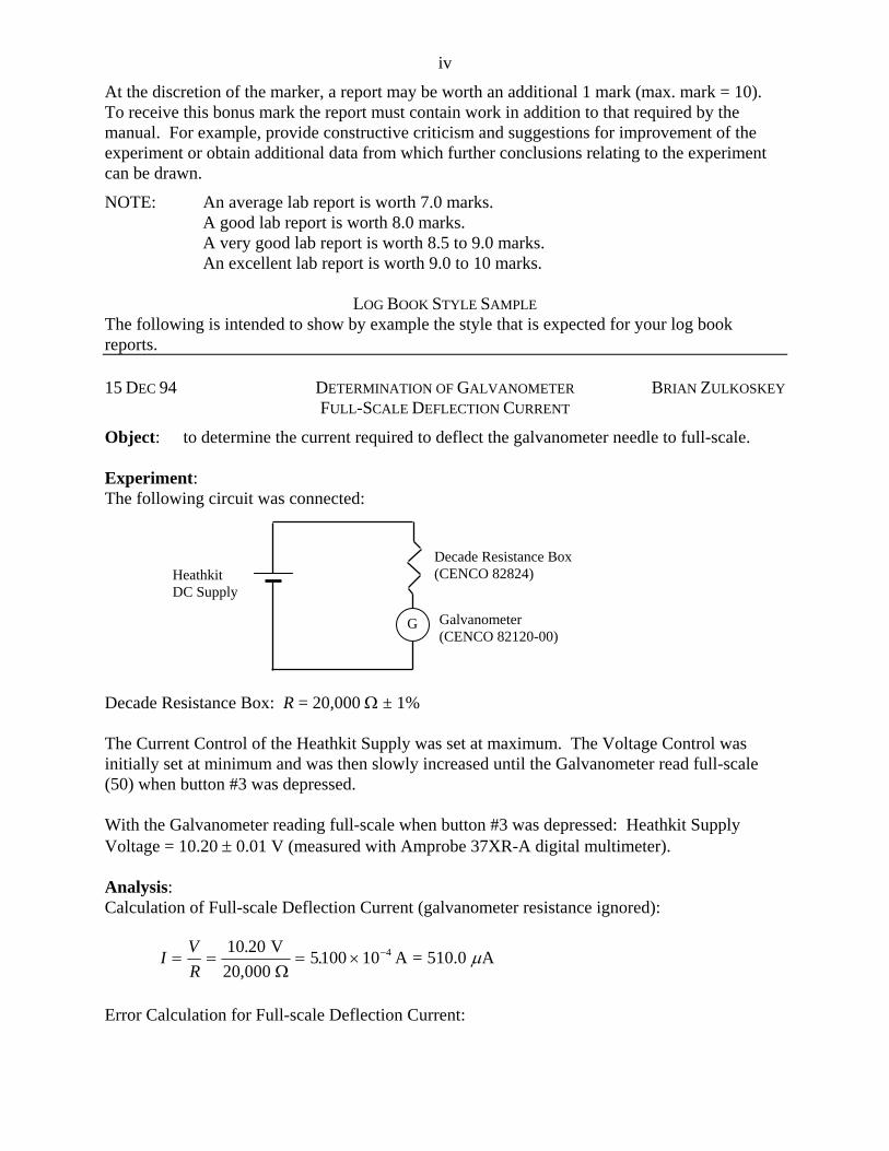
LOG BOOK STYLE SAMPLE The following is intended to show by example the style that is expected for your log book reports. 15 DEC 94 DETERMINATION OF GALVANOMETER BRIAN ZULKOSKEY FULL-SCALE DEFLECTION CURRENT
Object: to determine the current required to deflect the galvanometer needle to full-scale. Experiment: The following circuit was connected: Decade Resistance Box: R = 20,000 ± 1% The Current Control of the Heathkit Supply was set at maximum. The Voltage Control was initially set at minimum and was then slowly increased until the Galvanometer read full-scale (50) when button #3 was depressed. With the Galvanometer reading full-scale when button #3 was depressed: Heathkit Supply Voltage = 10.20 0.01 V (measured with Amprobe 37XR-A digital multimeter). Analysis: Calculation of Full-scale Deflection Current (galvanometer resistance ignored):
IV
R 10 20
20 0005100 10 4.
,.
VA = 510.0 A
Error Calculation for Full-scale Deflection Current:
G
Heathkit DC Supply
Decade Resistance Box (CENCO 82824)
Galvanometer (CENCO 82120-00)

v
A5.1=A100.051=A101.5
)000,20(
200)V20.10(
000,20
V01.0))(()(
4-6
2
2
22
2
22221
1
I
R
RV
R
VRRVRVI
VRR
VI
The experimental value obtained for the galvanometer full-scale deflection current is 510.0 ± 5.1 A. Conclusion: The experimental value of 510.0 ± 5.6 A is reasonably close to the quoted nominal value of 500 A for the galvanometer full-scale deflection current. Using a simple circuit and Ohm’s Law enabled determination of one of the galvanometer parameters that must be known in order to use the galvanometer as a measuring instrument. Sources of Error: All of the errors in this procedure are expected to have small effects on the result. – if the galvanometer is not properly zeroed the measured full-scale current value will be too
large or too small depending on which side of 0 the needle initially lies (systematic error). – mechanical friction in the needle suspension may cause varying needle response (random
error). – judgement error in deciding when the meter is reading exactly full-scale (random error). – to account for possible variations in the meter response due to ‘direction of deflection’-
dependent mechanical properties, the full-scale deflection currents should have been determined for the meter deflecting to each side of 0, and the results averaged.

vi
C: GRAPHICAL REPRESENTATION AND INTERPRETATION OF EXPERIMENTAL DATA
In order to understand a physical problem, one usually studies the dependence of one quantity upon another. Whereas sometimes such a dependence is obtained theoretically, at times it must be arrived at experimentally. The experimental determination involves obtaining experimentally a series of values of one quantity corresponding to the various arbitrary values of the other and then subjecting the data to some kind of analysis. One of the most convenient and useful means of treating the experimental data is by graphical analysis.
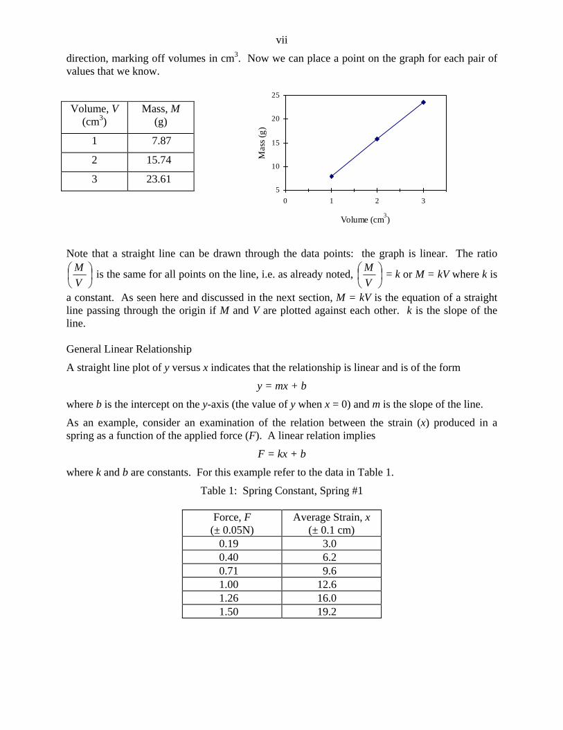
A graph shows the relation between the two quantities in the form of a curve. Suppose we are interested in looking at the relation between the volume of a piece of iron and its mass. If we make measurements on pieces of iron, we find that 1 cm3 has a mass of 7.87 g, 2 cm3 has a mass of 15.74 g, 3 cm3 has a mass of 23.61 g, and so on. This kind of relation in which doubling the volume doubles the mass, tripling the volume triples the mass, is called direct proportion. In Physics you will encounter many cases of such relations. In describing this relation we say:
(i) mass ‘is directly proportional to’ volume of iron or mass ‘varies directly as’ the volume of iron.
(ii) Mathematically we can write the relation as M V, where M is the mass of a piece of iron and V is its volume and the symbol means ‘is proportional to’. If we have two different volumes of iron, V1 and V2, their masses M1 and M2 may be expressed as
2
1
2
1
V
V
M
M
Another form of this relation expresses the fact than when mass and volume are related by direct proportion, they have a constant ratio. Thus
V
M of one sample =
V
M of another sample = k
The constant k is called the proportionality constant. In our example of iron
k = 7.87 g for each cubic centimetre
We now express this relation as an equation for any piece of iron:
V
M = k or M = kV, where the value of k as determined experimentally is 7.87 g/cm3.
An equation established in this way is an empirical equation.
We can illustrate this relation between mass and volume for iron by a graph. In trying to study the mass of a piece of iron as a function of its volume, we chose certain values for the volume and determined the corresponding values for the mass. In such a situation volume is said to be the independent variable and the mass is the dependent variable. Generally, the independent variable should be the variable that is altered in regular steps in the experiment, and the dependent variable is the quantity which is measured for each regular step of the independent variable. The independent variable (in our case the volume of a piece of iron) is plotted along the x axis and the dependent variable (in our case, the mass of the piece of iron) is plotted along the y axis. To plot the data we must choose scales – one for the vertical direction, marking off some suitable number of grams for each vertical division of the paper, and one for the horizontal
vii
direction, marking off volumes in cm3. Now we can place a point on the graph for each pair of values that we know.
Volume, V (cm3)
Mass, M (g)
1 7.87
2 15.74
3 23.61
Note that a straight line can be drawn through the data points: the graph is linear. The ratio
V
M is the same for all points on the line, i.e. as already noted,
V
M = k or M = kV where k is
a constant. As seen here and discussed in the next section, M = kV is the equation of a straight line passing through the origin if M and V are plotted against each other. k is the slope of the line. General Linear Relationship
A straight line plot of y versus x indicates that the relationship is linear and is of the form
y = mx + b
where b is the intercept on the y-axis (the value of y when x = 0) and m is the slope of the line.
As an example, consider an examination of the relation between the strain (x) produced in a spring as a function of the applied force (F). A linear relation implies
F = kx + b
where k and b are constants. For this example refer to the data in Table 1.
Table 1: Spring Constant, Spring #1
Force, F (± 0.05N)
Average Strain, x (± 0.1 cm)
0.19 3.0 0.40 6.2 0.71 9.6 1.00 12.6 1.26 16.0 1.50 19.2
5
10
15
20
25
0 1 2 3
Volume (cm3)
Mas
s (g
)

viii
(x4, y4) = (19.2 cm, 1.55 N) (x2, y2) = (17.8 cm, 1.40 N)
N/m8.33N/cm0833.0
cm0.12
N00.1
cm8.5cm8.17
N40.0N40.1
slope12
12
xx
yy
N/m8.70N/cm0870.0
cm2.16
N41.1
cm0.3cm2.19
N14.0N55.1
slopemax34
34
xx
yy
(slope) = max slope – slope slope = 8.33 ± 0.37 N/m = 8.70 N/m – 8.33 N/m = 0.37 N/m (x1, y1) = (5.8 cm, 0.40 N) (x3, y3) = (3.0 cm, 0.14 N)
Average Strain, x (cm)
Graph 1: Force vs. Average Strain to determine Spring Constant
For
ce, F
(N
)
ix
The experimentally obtained points usually do not lie exactly on a straight line; this is expected, because experimental data are never exact. In a straight line plot of experimental results, the straight line goes above some points and below others and represents an honest attempt on the part of the plotter to show the trend of the data. See Graph 1.
If the plot of y versus x yields a straight line, the relationship is linear and is of the form
y = mx + b
If m = 0, y does not depend on x. If the plot is a straight line passing through the origin, b = 0.
If the graph directly relating the variables does not give a straight line, one may search for the form of the function by considering a few of the common types of relationships one by one.
Power Relationship
One common type of relationship is of the form
u = cVn
where u and V are variables, c is a constant and n is the (constant) power to which V is raised and may be integral, fractional, positive, or negative. Taking logs of both sides gives
log u = log c + n log V
Letting log u = y, log c = b, and log V = x the equation becomes
y = nx + b
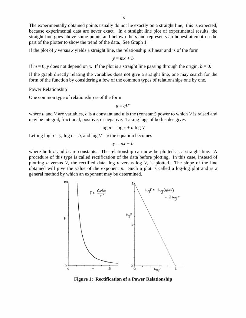
where both n and b are constants. The relationship can now be plotted as a straight line. A procedure of this type is called rectification of the data before plotting. In this case, instead of plotting u versus V, the rectified data, log u versus log V, is plotted. The slope of the line obtained will give the value of the exponent n. Such a plot is called a log-log plot and is a general method by which an exponent may be determined.
Figure 1: Rectification of a Power Relationship
x
Consider Newton's Law of Gravitation (2r
MmGF ). As shown in Figure 1, the plot of F versus
r does not clearly show the functional relationship between F and r. An inspection of the plot of log F versus log r shows a slope of –2 and thereby indicates the inverse square relation.
Exponential Relationship
Some physical situations are described by an exponential relationship. Such relationships are most commonly written as powers of the number e (= 2.71828...), the base of natural logarithms.
Consider the general form of an exponential relationship: axceu where c and a are constants.
Taking logarithms to the base e (ln) of both sides of the equation gives
ln u = ln c + ax
Since c is a constant, ln c is also a constant, and therefore a plot of ln u versus x will be a straight line with slope a and y-intercept ln c. Such a plot is called a semi-log plot.
This type of relationship is illustrated by the following example:
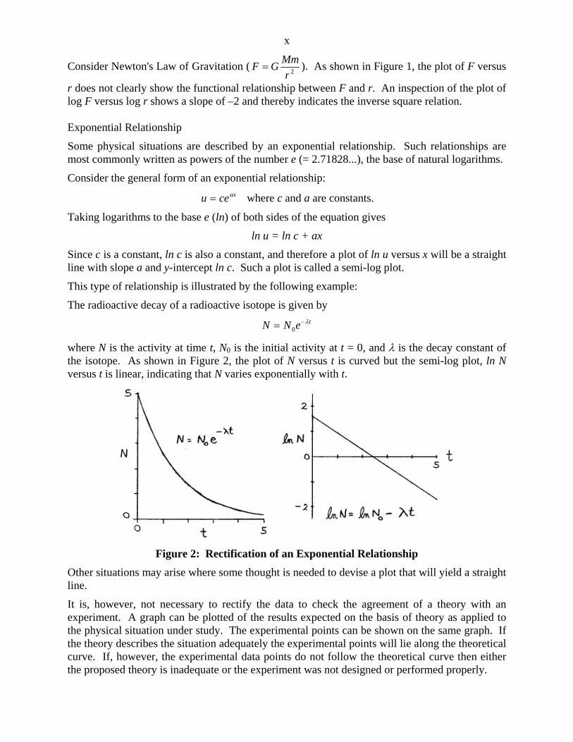
The radioactive decay of a radioactive isotope is given by teNN 0
where N is the activity at time t, N0 is the initial activity at t = 0, and is the decay constant of the isotope. As shown in Figure 2, the plot of N versus t is curved but the semi-log plot, ln N versus t is linear, indicating that N varies exponentially with t.
Figure 2: Rectification of an Exponential Relationship
Other situations may arise where some thought is needed to devise a plot that will yield a straight line.
It is, however, not necessary to rectify the data to check the agreement of a theory with an experiment. A graph can be plotted of the results expected on the basis of theory as applied to the physical situation under study. The experimental points can be shown on the same graph. If the theory describes the situation adequately the experimental points will lie along the theoretical curve. If, however, the experimental data points do not follow the theoretical curve then either the proposed theory is inadequate or the experiment was not designed or performed properly.
xi
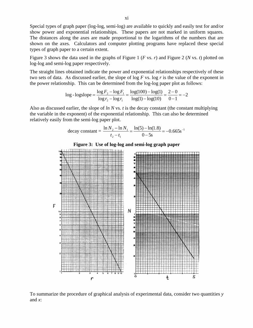
Special types of graph paper (log-log, semi-log) are available to quickly and easily test for and/or show power and exponential relationships. These papers are not marked in uniform squares. The distances along the axes are made proportional to the logarithms of the numbers that are shown on the axes. Calculators and computer plotting programs have replaced these special types of graph paper to a certain extent.
Figure 3 shows the data used in the graphs of Figure 1 (F vs. r) and Figure 2 (N vs. t) plotted on log-log and semi-log paper respectively.
The straight lines obtained indicate the power and exponential relationships respectively of these two sets of data. As discussed earlier, the slope of log F vs. log r is the value of the exponent in the power relationship. This can be determined from the log-log paper plot as follows:
210
02
)10log()1log(
)1log()100log(
loglog
loglogslopelog-log
12
12
rr
FF
Also as discussed earlier, the slope of ln N vs. t is the decay constant (the constant multiplying the variable in the exponent) of the exponential relationship. This can also be determined relatively easily from the semi-log paper plot.
decay constant = 1
12
12 s665.0s50
)8.1ln()5ln(lnln
tt
NN
Figure 3: Use of log-log and semi-log graph paper
To summarize the procedure of graphical analysis of experimental data, consider two quantities y and x:

xii
(a) If the plot of y versus x is a random scatter of points, y is not solely dependent on x in a smooth manner.
(b) If the plot of y versus x yields a straight line, the relationship is linear and is of the form y = mx + b. If m = 0, y does not depend on x. If the plot is a straight line passing through the origin, b = 0.
(c) If the plot of y versus x is not a straight line but log y versus log x yields a straight line then the relationship is that of a power law, the form being y = cxn.
(d) If the plot of ln y (or log y) versus x is a straight line then the relationship has an exponential form y = ceax. It may be necessary in practice to try plotting the log of one quantity versus the second quantity, and then the log of the second quantity versus the first.
When drawing graphs, the following rules are to be observed in order that the graphs neatly and clearly represent the experimental data.
1. Draw the axes. Axes are not normally placed along the boundaries between the graph paper and the margin although in some cases it may be necessary to do so because of the extent of the graph. Axes are usually drawn one or two large divisions in from the left and up from the bottom margin respectively. Label each axis with the variable being plotted (e.g. mass, period, time, etc.) and the units.
2. Mark the scales along the axes. The following points should be considered in choosing the scale:
a) the graph should be easy to read and it should be possible to easily interpolate values without the need for a calculator. Make each large division equal to 1, 2, 4, 5 or 10 units. Do NOT use scales of 3, 6, 7, 9, ... units per division;
b) the resultant curve should fill the whole graph and should not be confined to a small area of the graph paper;
c) the geometrical slope of the curve (if it is a straight line) should be approximately unity;
d) the point (0, 0) should not appear on the scales unless the point (0, 0) is a significant point on the graph.
3. Plot the points carefully. Mark each point so that the plotted point stands out clearly. When two sets of different data are plotted on the same set of axes use different symbols (e.g. circles and crosses) for each set of data.
4. Fit a curve to the plotted points. Most of the graphs drawn will be for the purpose of illustrating a law or determining a relationship. Hence it is reasonable to assume that the graph should be a uniformly smooth curve, possibly a straight line. Owing to the limits of experimental accuracy not all the plotted points will be exactly on the smooth curve or straight line. Use a transparent French curve or straight edge and draw a curve through the plotted points so that:
a) the curve is smooth;
b) the curve passes as close as possible to all the data points;
c) when taken in moderately sized groups, as many points fall on one side of the curve as on the other.
Note that the curve need not pass through any one point, and certainly need not pass through the end points as these end points are usually obtained at the limits of the accuracy of the

xiii
measuring instrument. Use dashes to show the extrapolation of the curve past the range of the data points.
5. Give the completed graph a descriptive title (what is being plotted and why). This should be placed in a position where it does not interfere with the curve.
6. If a slope calculation is required it should be done on the graph page or on the page immediately following the graph page. This reduces the possibilities of error in slope calculations and makes interpretation of the graph easier. A LARGE triangle should be drawn on the graph with vertices (x1, y1) and (x2, y2) as shown in Graph 1. The vertices are then used to calculate the slope according to the formula:
x
y
xx
yy
12
12
run
riseslope
Data points should not be used in slope calculations.
The experimental error in the slope can be calculated by performing an error calculation (discussed in a later section) on the slope equation.
7. It is sometimes desirable to indicate the experimental error in the plotted data points (see the section Discussion of Errors). This is done with ERROR BARS, which are shown in Graph 1. Vertical error bars are drawn by going above and below a data point a distance, determined by the vertical scale, corresponding to the error in the y-value. Horizontal error bars are drawn by going on either side of the data point a distance corresponding to the error in the x-value.
When error bars are drawn, the experimental error in the slope of a straight line is determined by one of the following methods:
Method 1
a) as already discussed, the best-fit straight line is drawn and its slope is calculated;
b) another line is drawn on the graph, this EXTREME-FIT line is the line passing through or near the error bars of all the data points and having the maximum or minimum possible slope;
c) the error in the best-fit slope is then taken as the absolute value of the difference between the extreme-fit slope and the best-fit slope.
Method 2
a) both the maximum-slope and the minimum-slope EXTREME-FIT lines are drawn on the graph;
b) the average slope is taken as the average of the slopes of the maximum-fit and minimum-fit lines;
c) the error in the average slope is taken as half the difference between the maximum-fit slope and the minimum-fit slope.
2
min)(max)(;
2
min)(max
slopeavgslopeavg
D: DISCUSSION OF ERRORS
xiv
Accuracy of Physical Measurements
Whether an experiment is of a precision type in which the answer is the magnitude of a quantity or of a qualitative nature in which the main aim is to substantiate a qualitative conclusion, it always involves taking measurements. Every measurement of a physical quantity is uncertain by some amount. When an observation or a result is recorded, one may ask the question - how precisely do we know this quantity? What we are asking for is a statement of some range of confidence in the quoted value or an expression of the uncertainty, sometimes called the error, in the quantity. By the word error we do not mean mistake but rather the uncertainty in the quantity.
There are three types of errors that may occur in experimental work:
1. Blunders or Mistakes on the part of the observer in reading the instruments or recording observations can be avoided by the exercise of reasonable care and therefore need no discussion. Some simple rules that will reduce the possibility of such mistakes are:
(a) consider whether or not the reading taken is reasonable. Is it of the order of magnitude expected?
(b) record the reading immediately and directly in the laboratory notebook. Do not attempt to remember it even for a few minutes nor record it on a loose sheet;
(c) whenever possible have your partner check your reading.
2. Systematic Errors refer to uncertainties that influence all the measurements of a particular quantity equally. These errors may be inherent in the calibration of a particular instrument or in the particular design of the apparatus used. For example, the reading on a certain thermometer may be consistently too high because the thermometer was incorrectly calibrated. Systematic errors can usually be eliminated either by calibrating the particular instrument under conditions similar to those of the experiment or by applying a correction term in the calculations. In those cases where it is known to be necessary to apply a correction for a systematic error in the experiments performed in this laboratory, the instructors will give the details of the procedure to be followed.
3. Experimental or Random Errors remain even when all mistakes and systematic errors have been avoided or accounted for. Thus when a given measurement is repeated the resulting values, in general, do not agree exactly. No one has so far designed a perfect experiment: imperfections in our senses; in the instruments we use; and chance variations in conditions assumed to remain constant all combine to cause uncertainties in our measurements. These random errors are unavoidable and their exact magnitude cannot be determined.
A good example of these random deviations or accidental errors is provided by the shot pattern obtained when an accurately zeroed and solidly clamped rifle is fired at a target. The pattern of fire will show a scatter of shots about the centre of fire, the number of shots in a given annular ring of constant width being progressively less as the distance from the centre of fire increases. The same effect may be demonstrated by repeatedly dropping a dart or sharp-pointed pencil vertically onto a mark on a piece of paper. The scatter of the shots about the aiming mark is analogous to the spread of experimentally obtained values about their mean value, due to accidental errors.
It is often difficult to determine the magnitude of systematic errors in an experiment. For example, in the case discussed of a systematic error introduced by a poorly calibrated thermometer one doesn't know if the error is 1° or 10° unless the thermometer is compared to a reliable thermometer. In the case of random errors, however, the data taken in the experiment is enough to indicate how large these errors are.

xv
A common way of approximating the magnitude of random errors is the use of significant figures. For a more reliable estimate of these errors, statistical methods and error calculations are employed.
xvi
E: SIGNIFICANT FIGURES
Numerical quantities have a different meaning in physics than they do in mathematics. The term ‘significant figures’ refers to the fact that while to a mathematician numbers are exact quantities, to a physicist a number is often a measured quantity and therefore inexact. A rough approximation of the uncertainty or experimental error in a number is indicated by the physicist by only writing those figures of the number in which he/she has confidence, i.e. by only writing the figures that are significant. For example, to a mathematician, 16 is the same as 16.0 or 16.00, but to a physicist, if x is a length measurement then x = 16 cm means 15.5 cm < x < 16.5 cm; x = 16.0 cm means 15.95 cm < x < 16.05 cm; and x = 16.00 cm means 15.995 cm < x < 16.005 cm.
Note that zeros used as place holders between the decimal point and the number are not significant and that zeros after the number may or may not be significant. To avoid this possible source of confusion very large and very small numbers are often written in scientific notation (also called power of ten notation). In this notation the number is written with one figure to the left of the decimal point and then multiplied by the appropriate power of ten.
e.g. 001804 = 1.804 × 10⁻³ (4 sig. fig.)
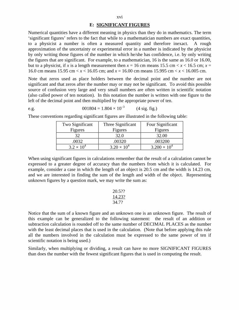
These conventions regarding significant figures are illustrated in the following table:
Two Significant Figures
Three Significant Figures
Four Significant Figures
32 32.0 32.00 .0032 .00320 .003200
3.2 × 10⁴ 3.20 × 10⁴ 3.200 × 10⁴ When using significant figures in calculations remember that the result of a calculation cannot be expressed to a greater degree of accuracy than the numbers from which it is calculated. For example, consider a case in which the length of an object is 20.5 cm and the width is 14.23 cm, and we are interested in finding the sum of the length and width of the object. Representing unknown figures by a question mark, we may write the sum as: 20.5?? 14.23? 34.7? Notice that the sum of a known figure and an unknown one is an unknown figure. The result of this example can be generalized to the following statement: the result of an addition or subtraction calculation is rounded off to the same number of DECIMAL PLACES as the number with the least decimal places that is used in the calculation. (Note that before applying this rule all the numbers involved in the calculation must be expressed to the same power of ten if scientific notation is being used.)
Similarly, when multiplying or dividing, a result can have no more SIGNIFICANT FIGURES than does the number with the fewest significant figures that is used in computing the result.

xvii
Exercises on Significant Figures
1. How many significant figures do each of the following numbers have? (a) 6.3 × 10³ (b) .00370 (c) 6700 (d) 670.0 × 10³
2. Round off to 2 significant figures and express in scientific notation: (a) 3.95 (b) .02862 (c) 219 (d) 4326
3. Calculate to the appropriate number of significant figures and express in scientific notation: (a) 63400 + 82 (b) 480 ÷ .060 (c) 379 – (6 × 10³) (d) 8900 ÷ 30 (e) 290 + 6.7 (f) .030 – .003 (g) 321 × 3
4. Suppose that you are instructed to draw a line ten centimetres long using an ordinary ruler (one which has millimetres marked on it). How will the length of the line be best expressed?
(a) 1 × 101 cm (b) 10 cm (c) 10.0 cm (d) 10.00 cm

xviii
F: ESTIMATING ABSOLUTE ERRORS FROM RANDOM CAUSES
The ABSOLUTE error in a quantity is the estimate of the range of values to be expected due to experimental errors. The absolute error has the same units as the quantity and is denoted by the Greek symbol lower-case delta () in front of the symbol for the quantity. For example, if a length measurement is denoted by x then x is the absolute error in this length. Experimental error can also be expressed relative to the quantity. This RELATIVE error is defined as the absolute error divided by the quantity. In symbols the relative error would be x/x for the example mentioned above. If expressed as a percentage, the relative error becomes a PERCENTAGE error, and is calculated by (x/x) × 100%.
The correct use of significant figures gives a rough estimate of the magnitude of random errors involved in taking readings. A more precise and reliable method of determining random errors is to determine absolute errors by estimation or calculation and then to use these values in subsequent calculations. Generally speaking, calculated values can be no more precise than the individual measurements. In fact, the errors accumulate so that the calculated value is usually less precise than the measurements on which it is based. The errors in a calculated quantity can be determined from the errors in each of the directly measured quantities on which the calculation is based. Before proceeding to calculate the experimental error, however, we must decide what numerical value shall be given to the absolute error in any measurement. The following rules may be used for assigning absolute errors:
1. When a quantity is just measured once, the measured value is taken as being the ‘true’ value and the absolute error due to random causes is estimated as the MAXIMUM INSTRUMENTAL ERROR in the measuring instrument. The maximum instrumental error will usually be the least count of the instrument (the size of the smallest scale division). For example in measuring the length of an object with a meter stick, the error would be ±1 mm since 1 mm is the smallest scale division on the meter stick.
2. A more accurate estimate of error can be obtained when a quantity is measured several times. The effect of random errors is usually to cause measurements to be distributed according to a normal curve (also called a bell-shaped or a Gaussian curve). An example of such a distribution would be obtained by a person shooting billiard balls at a meter stick placed at the edge of a billiard table. If he/she aimed at the 50 cm mark then his/her record of hits after many trials might look like the following:

xix
This bell-shaped distribution is caused by random errors: errors such as irregular wind currents, lack of sphericity in the billiard balls, etc. Note that the effect of a systematic error would be quite different. If the table was not level, for example, one might obtain a bell-shaped distribution around the 55 cm mark but the shape of the curve would be unchanged.
It is beyond the scope of this class to enter into a complete discussion of the statistical methods but the main results of the analysis of normal curves are as follows:
(a) The 'best' or most probable value in a normal distribution is the arithmetic mean x
xn
xii
n
1
1
where x1, x2, ..., xn are the individual measurements and n is the number of measurements.
(b) To provide a measure of the error in the measurement, one defines a quantity called the STANDARD DEVIATION IN THE MEAN:
x
1
12
1n nx xi
i
n
( )( )
For a normal distribution the probability of obtaining an error in x less than ± is 68.2%. In other words, on an average of 68 times out of 100 the true value of the quantity being measured will fall within the range of x – to x + . The probability of an error less than ±2 is 95.4% and the probability of an error less than ±3 is 99.7%.
Note that this method of treating errors has the following limitations: it assumes a normal distribution which is usually but not always valid; it provides no indication of errors due to systematic causes; the above formula is not the same as the formula used for standard deviation on most calculators.
The suggested procedure for this course will be to quote the error as x with 68% confidence. However, if the instrument error as described in 1. is greater than , then the instrument error should be taken to be the absolute error.

xx
G: PROPAGATION OF ERRORS IN CALCULATIONS In a number of cases the quantity of interest cannot be measured directly – it is calculated by using two or more directly measured quantities. When uncertain quantities are used in numerical calculations one usually wishes to know the error in the result. The simplest method, although not the most accurate, is to determine the maximum possible error. MAXIMUM POSSIBLE ERROR METHOD
CALCULUS TECHNIQUE
One technique for obtaining an error expression is to make use of calculus. If you are familiar with the rules for derivatives you will find this technique relatively simple.
Bottom Line: The maximum experimental uncertainty in a calculated value is obtained by adding the absolute values of the terms arising from the partial differential of the expression for the calculated value, treating each measured value as a variable.
Details: Before proceeding, a brief review of some of the definitions and rules of differential calculus will be helpful.
Suppose y is some function of the variable x. Then the derivative of y with respect to x is dy/dx, sometimes denoted y'. Mathematicians speak of ‘d/dx’ as being the differentiation operator: ‘d( )/dx’ means ‘take the derivative with respect to x’ of whatever function is placed in the parentheses. ‘d( )/dx’ can also be considered to represent the small change d( ) that occurs in ( ), for a small change dx in x, divided by this small change in x.
Therefore, starting from
dy
dxy
and multiplying both sides by the small change dx in x, yields
dy = y dx
Therefore the small change in the variable y arising from a small change in the variable x is calculated by multiplying the small change in x by the derivative of y with respect to x.
The ‘small changes’ are called the DIFFERENTIALS of the appropriate variables.
The rules of calculus for calculating differentials are the same as those for calculating derivatives.
Suppose y = cxn,
Using the exponent rule, the DERIVATIVE of y with respect to x, dy/dx = y', is
dy
dxy ncx n 1
The DIFFERENTIAL of y is
dy = ncxn–1 dx
Similarly, if u, v, and w are functions of some (dummy) variable x:

xxi
d
dxu v w
du
dx
dv
dx
dw
dx( ) (derivative)
d(u + v – w) = du + dv – dw (differential)
d
dxuvw vw
du
dxuw
dv
dxuv
dw
dx( ) (derivative)
d(uvw) = vw du + uw dv + uv dw (differential)
d
dxu
vv du dx u dv dx
v
( / ) ( / )2
(derivative)
d uv
vdu udv
v
2
(differential)
d
dx
d
dx(sin ) cos
(derivative)
d(sin) = cos d (differential)
Application of these rules of calculus to calculation of errors proceeds as follows:
1. Ensure that the original expression is in its simplest form and that each variable is independent of all other variables. You may also find it easier if you replace division with multiplication and negative exponents. e.g. replace a/b with ab–1.
2. Calculate the differential of the expression. (Each symbol representing a measured value is taken as a variable to be differentiated.)
3. Take the absolute value of each term in the differential expression. A TERM is defined as an expression containing ONE differential quantity. e.g. (a/b) dx, uvw dx, y dv, (a–b) dx. The expression (dx – dy) is TWO terms:
(dx – dy) = dx – dy = dx + (–dy)
The effect of this rule is that (dx – dy) becomes
|dx| + |–dy| = dx + dy
i.e. The terms in the differential expression add.
4. Whenever the differential of any variable appears, substitute the absolute error of that variable.
5. When angles are used, the absolute error of the angle must be expressed in radians (not degrees).
The following examples illustrate this technique.
Example 1
The equation for kinetic energy is KE = 12 mv2 where m and v are mass and speed respectively.
The differential of KE is:
dKE = 12 dm v2 + 1
2 m 2v dv
Thus the absolute error of K is:
KE = 12 m v2 + 1
2 m 2v v
xxii
where m and v are the absolute errors in m and v.
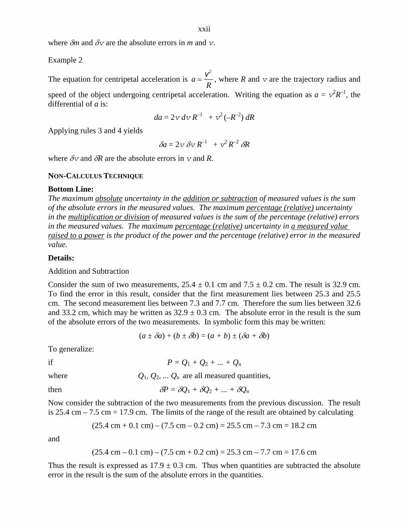
Example 2
The equation for centripetal acceleration is aR
v2
, where R and v are the trajectory radius and
speed of the object undergoing centripetal acceleration. Writing the equation as a = v2R–1, the differential of a is:
da = 2v dv R–1 + v2 (–R–2) dR
Applying rules 3 and 4 yields
a = 2v v R–1 + v2 R–2 R
where v and R are the absolute errors in v and R.
NON-CALCULUS TECHNIQUE
Bottom Line: The maximum absolute uncertainty in the addition or subtraction of measured values is the sum of the absolute errors in the measured values. The maximum percentage (relative) uncertainty in the multiplication or division of measured values is the sum of the percentage (relative) errors in the measured values. The maximum percentage (relative) uncertainty in a measured value raised to a power is the product of the power and the percentage (relative) error in the measured value.
Details:
Addition and Subtraction
Consider the sum of two measurements, 25.4 ± 0.1 cm and 7.5 ± 0.2 cm. The result is 32.9 cm. To find the error in this result, consider that the first measurement lies between 25.3 and 25.5 cm. The second measurement lies between 7.3 and 7.7 cm. Therefore the sum lies between 32.6 and 33.2 cm, which may be written as 32.9 ± 0.3 cm. The absolute error in the result is the sum of the absolute errors of the two measurements. In symbolic form this may be written:
(a ± a) + (b ± b) = (a + b) ± (a + b)
To generalize:
if P = Q1 + Q2 + ... + Qn
where Q1, Q2, ... Qn are all measured quantities,
then P = Q1 + Q2 + ... + Qn
Now consider the subtraction of the two measurements from the previous discussion. The result is 25.4 cm – 7.5 cm = 17.9 cm. The limits of the range of the result are obtained by calculating
(25.4 cm + 0.1 cm) – (7.5 cm – 0.2 cm) = 25.5 cm – 7.3 cm = 18.2 cm
and
(25.4 cm – 0.1 cm) – (7.5 cm + 0.2 cm) = 25.3 cm – 7.7 cm = 17.6 cm
Thus the result is expressed as 17.9 ± 0.3 cm. Thus when quantities are subtracted the absolute error in the result is the sum of the absolute errors in the quantities.
xxiii
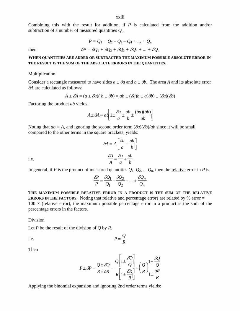
Combining this with the result for addition, if P is calculated from the addition and/or subtraction of a number of measured quantities Qi,
P = Q1 + Q2 – Q3 – Q4 + ... + Qn
then P = Q1 + Q2 +Q3 + Q4 + ... + Qn
WHEN QUANTITIES ARE ADDED OR SUBTRACTED THE MAXIMUM POSSIBLE ABSOLUTE ERROR IN
THE RESULT IS THE SUM OF THE ABSOLUTE ERRORS IN THE QUANTITIES. Multiplication
Consider a rectangle measured to have sides a ± a and b ± b. The area A and its absolute error A are calculated as follows:
A±A = (a ± a)( b ± b) = ab ± (a)b ± ab) ± (a)b)
Factoring the product ab yields:
A A aba
a
b
b
a b
ab
1( )( )
Noting that ab = A, and ignoring the second order term (a)(b)/ab since it will be small compared to the other terms in the square brackets, yields:
A A
a
a
b
b
i.e. A
A
a
a
b
b
In general, if P is the product of measured quantities Q1, Q2, ... Qn, then the relative error in P is
P
P
Q
Q
Q
Q
Q
Qn
n 1
1
2
2
THE MAXIMUM POSSIBLE RELATIVE ERROR IN A PRODUCT IS THE SUM OF THE RELATIVE
ERRORS IN THE FACTORS. Noting that relative and percentage errors are related by % error = 100 × (relative error), the maximum possible percentage error in a product is the sum of the percentage errors in the factors. Division
Let P be the result of the division of Q by R.
i.e. PQ
R
Then
P PQ Q
R R
Q
RR
R
Q
R
Q
QR
R
1
1
1
1
Applying the binomial expansion and ignoring 2nd order terms yields:

xxiv
P PQ
R
Q
Q
R
RP
Q
Q
R
R
1 1
so
P PQ
Q
R
R
i.e. P
P
Q
Q
R
R
THE MAXIMUM POSSIBLE RELATIVE ERROR IN A QUOTIENT IS THE SUM OF THE RELATIVE
ERRORS IN THE DIVISOR AND DIVIDEND. Powers and Roots
Using the result obtained for multiplication and realizing that the expression Qn means to multiply Q by itself n times, if
P = Qn then
P
Pn
Q
Q
THE MAXIMUM POSSIBLE RELATIVE ERROR IN RAISING A BASE VALUE TO AN EXPONENT IS THE
PRODUCT OF THE EXPONENT AND THE RELATIVE ERROR IN THE BASE.
For a more general example, consider the quantity N given by the following expression:
N = (AB4)/(CD½)
where A, B, C, D are all measured quantities. The maximum possible relative error in N is
N
N
A
A
B
B
C
C
D
D 4 ½
Note that the error in N is influenced more by errors made in measuring B than any of the other quantities. In designing and performing such an experiment great care should be taken to measure B with the highest degree of precision attainable. SUMMARY
1. All measured quantities have associated with them an uncertainty which can be expressed as an absolute or relative error and which limits the number of significant figures of these quantities and any results calculated from them.
2. When uncertain quantities are added or subtracted the maximum possible absolute error of the result is determined by adding the absolute errors of the separate quantities.
3. When uncertain quantities are multiplied or divided the maximum possible relative error of the result is determined by adding the relative errors of the separate quantities.
4. When an uncertain quantity is raised to a power (including a fractional power) the maximum possible relative error in the result is determined by multiplying the relative error in the quantity by the exponent.
xxv
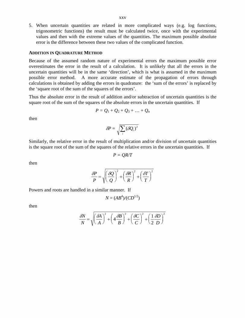
5. When uncertain quantities are related in more complicated ways (e.g. log functions, trigonometric functions) the result must be calculated twice, once with the experimental values and then with the extreme values of the quantities. The maximum possible absolute error is the difference between these two values of the complicated function.
ADDITION IN QUADRATURE METHOD
Because of the assumed random nature of experimental errors the maximum possible error overestimates the error in the result of a calculation. It is unlikely that all the errors in the uncertain quantities will be in the same ‘direction’, which is what is assumed in the maximum possible error method. A more accurate estimate of the propagation of errors through calculations is obtained by adding the errors in quadrature: the ‘sum of the errors’ is replaced by the ‘square root of the sum of the squares of the errors’.
Thus the absolute error in the result of addition and/or subtraction of uncertain quantities is the square root of the sum of the squares of the absolute errors in the uncertain quantities. If
P = Q1 + Q2 + Q3 + … + Qn
then
P = ( )Qii
2
Similarly, the relative error in the result of multiplication and/or division of uncertain quantities is the square root of the sum of the squares of the relative errors in the uncertain quantities. If
P = QR/T
then
P
P
Q
Q
R
R
T
T
2 2 2
Powers and roots are handled in a similar manner. If
N = (AB4)/(CD1/2)
then
N
N
A
A
B
B
C
C
D
D
2 2 2 2
41
2

xxvi
ERROR CALCULATION QUESTIONS
These questions are designed to help you in reviewing error calculations. In each of the questions you will be given an equation and some data to use in the equation. Each question consists of four parts.
(a) Derive the error equation. The error equation should be in symbols only.
(b) Use the data to do the calculation. Watch your significant figures and the units.
(c) Calculate the absolute error.
(d) Express the answer, with its absolute error, to the appropriate number of significant figures.
SAMPLE
The equation for kinetic energy is KE = 12 mv2 where m and v are mass and speed
respectively. Suppose that the following values were obtained in an experiment:
m = 5.32 ± 0.03 kg and v = 2.37 ± 0.07 m/s
(a) KE = 12 m v2 + 1
2 m 2v v where m and v are the absolute errors in m and v.
(b) KE = 12 (5.32 kg)(2.37 m/s)2 = 14.94 kgm2/s2 = 14.9 J
(c) KE = 12 (0.03 kg)(2.37 m/s)2 + 1
2 (5.32 kg)(2)(2.37 m/s)(0.07 m/s) = 0.967 J
(d) KE = 14.9 ± 1.0 J 1. The equation of an ellipse is
y bx
a= 1
2
2 ,
a = 22.6 ± 0.1 cm, b = 46.9 ± 0.1 cm, x = 12.2 ± 0.1 cm: y = 39.48 0.29 cm
2. From Kepler's third law of planetary motion, the orbital period T of a satellite in a circular
orbit at height h above a massive body of radius R and mass M is:
TR h
GM= 2
3
( ),
R = (1.738 ± 0.001) × 106 m; h = (1.1 ± 0.1) × 106 m
G = 6.67 × 10⁻¹¹ N·m2/kg2; M = (7.35 ± 0.01) × 1022 kg
T = (1.357 0.073) 104 s 3. Consider an Atwood's machine in which the pulley is neither frictionless nor massless. In
that case the acceleration is
am m g
I R m m m
( )
( / )2 1
21 2
where I is the moment of inertia of the pulley, R is its radius and m is a mass that is used to counteract the friction. Given g = 980 cm/s2, m1 = 100 ± 1 g, m2 = 200 ± 2 g,
I = 950 ± 50 g·cm2, R = 3.5 ± 0.1 cm and m = 5.0 ± 0.1 g: a = 256 15 cm/s2.

xxvii
4. When resistances R1, R2, and R3 are connected in parallel the total resistance, R, is given by
the equation
1 1 1 1
1 2 3R R R R
Given: R1 = 50 5 , R2 = 70 5 , R3 = 95 5 . R = 22.3 1.8

xxviii
H: SAMPLE CALCULATIONS For each different equation used in the analysis of an experiment a sample calculation (and possibly a sample error calculation) are required. The following discussion explains what is required in a proper sample calculation.
1. Label the calculation descriptively. Explicitly state, in words, what is being calculated. If this is one of many similar calculations, specify which one.
2. State the values, with their units and experimental errors, that will be used in the calculation. 3. State the equation in symbols. 4. Show the substitution of the values (with their units but not their experimental errors) into
the equation. 5. Give the result of the calculation. (Don’t round off, keep extra significant figures at this
stage, especially trailing zeros. Rounding will be done later). 6. State the error equation in symbols. 7. Show the substitution of values (with units) into the error equation. 8. Give the unrounded result of the error calculation, with units. 9. State the result and its absolute error with the appropriate number of significant figures.
The following rule is to be used in rounding off the results of calculations: ROUND OFF THE ABSOLUTE ERROR IN THE RESULT TO TWO SIGNIFICANT FIGURES, THEN ROUND OFF THE RESULT TO THE SAME NUMBER OF DECIMAL PLACES AS THE ABSOLUTE ERROR. If scientific notation is being used, express both the result and its absolute error to the same power of ten before applying the second part of this rule.
As an example, suppose the mass and speed of a car on an air track have been measured and the magnitude of the car’s momentum is to be calculated. The following is the correct sample calculation:
1. Sample Calculation of Momentum of Car (label) on Air Track for Trial #1
2. m = 0.675 ± 0.001 kg (statement of values) v = 0.123 ± 0.005 m/s
3. p = m (equation in symbols) 4. p = (0.675 kg)(0.123 m/s) (substitution of values) 5. p = 0.083025 kg·m/s (calculation result)
6. p = |m | + | m | (error equation in symbols)
7. p = (0.001 kg)(0.123 m/s) + (0.675 kg)(0.005 m/s) (substitution of values)
8. p = 0.003498 kg·m/s = 0.0035 kg·m/s (error calculation result)
9. p = 0.0830 ± 0.0035 kg·m/s or (round off) p = (8.30 ± 0.35) × 10–2 kg·m/s if scientific notation is being used
xxix
I: COMPARING TWO QUANTITIES
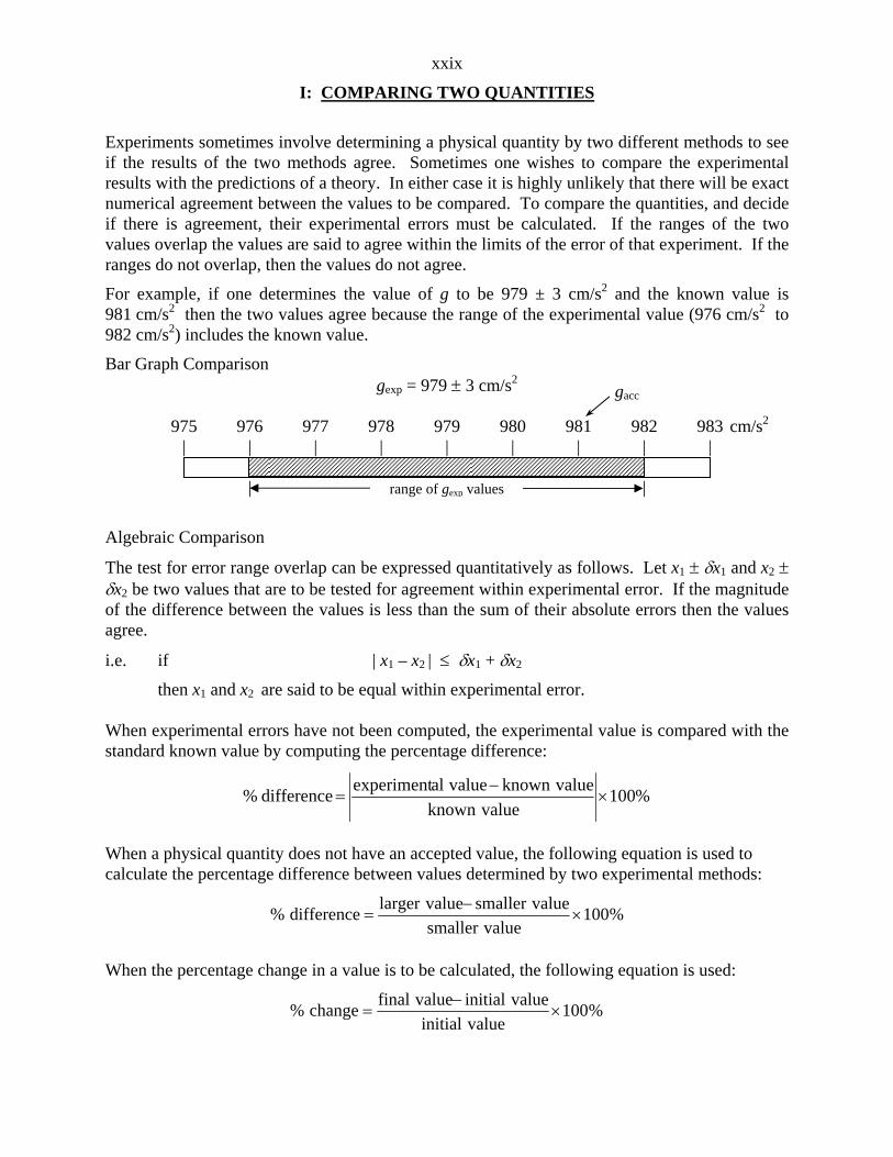
Experiments sometimes involve determining a physical quantity by two different methods to see if the results of the two methods agree. Sometimes one wishes to compare the experimental results with the predictions of a theory. In either case it is highly unlikely that there will be exact numerical agreement between the values to be compared. To compare the quantities, and decide if there is agreement, their experimental errors must be calculated. If the ranges of the two values overlap the values are said to agree within the limits of the error of that experiment. If the ranges do not overlap, then the values do not agree.
For example, if one determines the value of g to be 979 ± 3 cm/s2 and the known value is 981 cm/s2 then the two values agree because the range of the experimental value (976 cm/s2 to 982 cm/s2) includes the known value.
Bar Graph Comparison gexp = 979 3 cm/s2
975 976 977 978 979 980 981 982 983 cm/s2 | | | | | | | | | | |
Algebraic Comparison
The test for error range overlap can be expressed quantitatively as follows. Let x1 x1 and x2 x2 be two values that are to be tested for agreement within experimental error. If the magnitude of the difference between the values is less than the sum of their absolute errors then the values agree.
i.e. if | x1 – x2 | x1 + x2
then x1 and x2 are said to be equal within experimental error. When experimental errors have not been computed, the experimental value is compared with the standard known value by computing the percentage difference:
%100valueknown
valueknownvaluealexperimentdifference%
When a physical quantity does not have an accepted value, the following equation is used to calculate the percentage difference between values determined by two experimental methods:
%100valuesmaller
valuesmallervaluelargerdifference%
When the percentage change in a value is to be calculated, the following equation is used:
%100valueinitial
valueinitialvaluefinalchange%
range of gexp values
gacc

21 Jan 13 1 Phys 231 Expt 1
MIRRORS AND LENSES – GEOMETRIC OPTICS REVIEW AND ADDITIONAL THEORY Concave Mirror
Figure 1
Rfqpf 2
1;111
(1)
Quantity Positive when… Negative when… p object in front of mirror object in back of mirror q image in front image in back f and R concave mirror convex mirror h' (image height) image is upright image is inverted Thin Lenses When an object is viewed through a lens, the position of the image may be graphically determined by using principal rays. The method consists of propagating any two of the three principal rays from a point on the object and noting the point where they recombine after passing through the lens.
Figure 2
p (+)
f
q (+)
object
image
f (+) 1
2
3
21 Jan 13 2 Phys 231 Expt 1
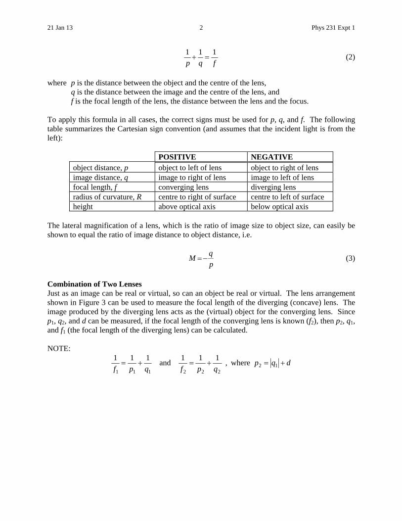
fqp
111 (2)
where p is the distance between the object and the centre of the lens, q is the distance between the image and the centre of the lens, and f is the focal length of the lens, the distance between the lens and the focus. To apply this formula in all cases, the correct signs must be used for p, q, and f. The following table summarizes the Cartesian sign convention (and assumes that the incident light is from the left):
POSITIVE NEGATIVE object distance, p object to left of lens object to right of lens image distance, q image to right of lens image to left of lens focal length, f converging lens diverging lens radius of curvature, R centre to right of surface centre to left of surface height above optical axis below optical axis
The lateral magnification of a lens, which is the ratio of image size to object size, can easily be shown to equal the ratio of image distance to object distance, i.e.
p
qM (3)
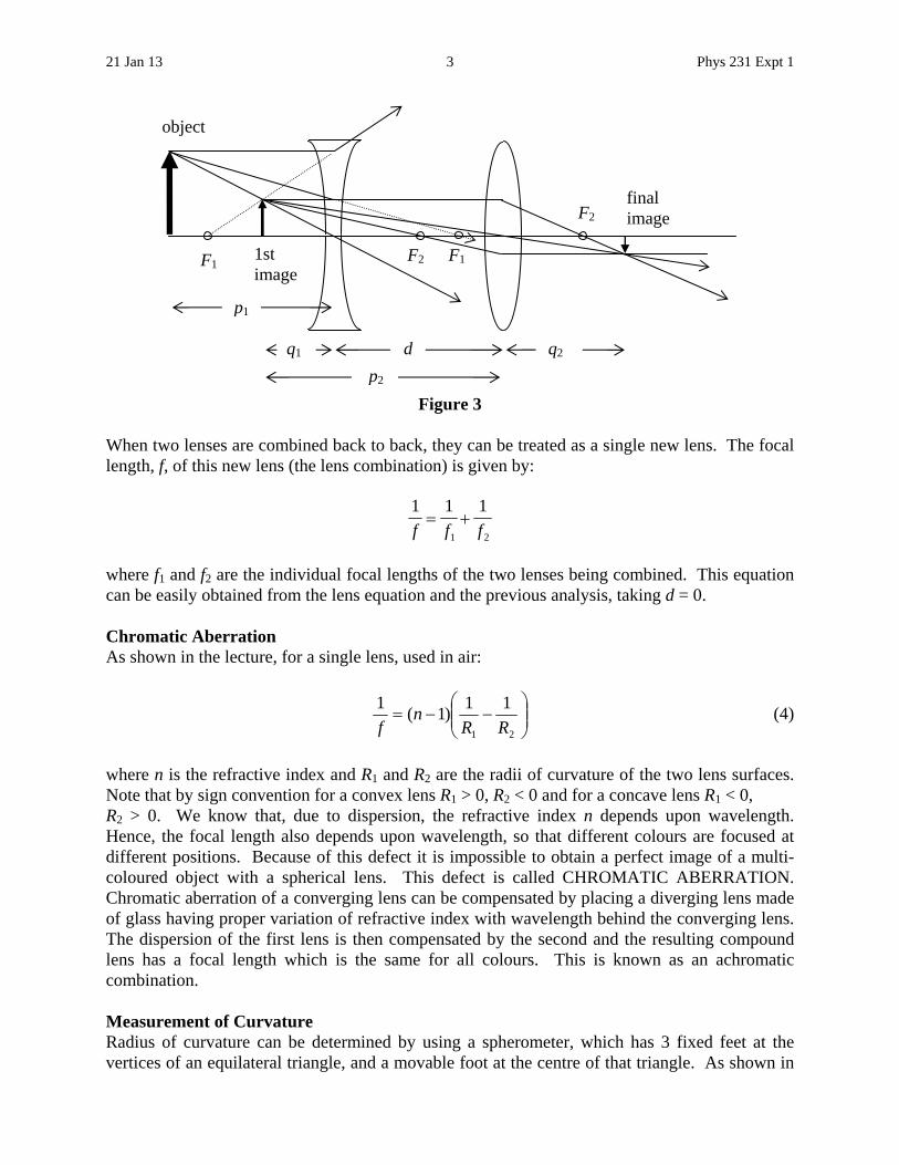
Combination of Two Lenses Just as an image can be real or virtual, so can an object be real or virtual. The lens arrangement shown in Figure 3 can be used to measure the focal length of the diverging (concave) lens. The image produced by the diverging lens acts as the (virtual) object for the converging lens. Since p1, q2, and d can be measured, if the focal length of the converging lens is known (f2), then p2, q1, and f1 (the focal length of the diverging lens) can be calculated. NOTE:
dqpqpfqpf
12222111
where, 111
and 111
21 Jan 13 3 Phys 231 Expt 1
Figure 3 When two lenses are combined back to back, they can be treated as a single new lens. The focal length, f, of this new lens (the lens combination) is given by:
1 1 1
1 2f f f
where f1 and f2 are the individual focal lengths of the two lenses being combined. This equation can be easily obtained from the lens equation and the previous analysis, taking d = 0. Chromatic Aberration As shown in the lecture, for a single lens, used in air:
21
11)1(
1
RRn
f (4)
where n is the refractive index and R1 and R2 are the radii of curvature of the two lens surfaces. Note that by sign convention for a convex lens R1 > 0, R2 < 0 and for a concave lens R1 < 0, R2 > 0. We know that, due to dispersion, the refractive index n depends upon wavelength. Hence, the focal length also depends upon wavelength, so that different colours are focused at different positions. Because of this defect it is impossible to obtain a perfect image of a multi-coloured object with a spherical lens. This defect is called CHROMATIC ABERRATION. Chromatic aberration of a converging lens can be compensated by placing a diverging lens made of glass having proper variation of refractive index with wavelength behind the converging lens. The dispersion of the first lens is then compensated by the second and the resulting compound lens has a focal length which is the same for all colours. This is known as an achromatic combination. Measurement of Curvature Radius of curvature can be determined by using a spherometer, which has 3 fixed feet at the vertices of an equilateral triangle, and a movable foot at the centre of that triangle. As shown in
q1
object
F2 F1
F2 final image
F1 1st image
p1
d q2
p2

21 Jan 13 4 Phys 231 Expt 1
Figure 4, the centre of the equilateral triangle is a distance 2y/3 from any corner, where y is the distance from a vertex to the midpoint of the opposite side. Since the length of a side of the triangle, a, is easily measured, it is convenient to express the distance 2y/3 in terms of the distance a: In triangle MNO:
y aa a
ya
2 22 2
4
3
4
3
2
hence
2
3 3
y a
Figure 4 Now imagine a vertical plane containing one of the fixed feet, the centre C of the equilateral triangle formed by the fixed feet, and the movable foot when it just touches the lens at height h above the point C. The radius of the curved surface is R. From the Pythagorean theorem:
32
3)(
2222
222
ahRhRR
ahRR
Solving for R:
h
ahR
62
2
Thus by measuring a and h, the radius of curvature, R, can be determined. EXPERIMENT The apparatus consists of an optical bench, a concave mirror, a converging lens, a diverging lens, a light source, an object slide, a screen, colour filters, and a spherometer. NOTE: Draw a ray diagram for each different mirror/lens/object situation (e.g. convex lens with p > f; etc.)

21 Jan 13 5 Phys 231 Expt 1
Object/Image data and results should be tabulated as follows:
Object Location ( __ cm)
Mirror/Lens Location ( __ cm)
Image Location
(cm)
p (cm)
q (cm)
f (cm)
Image Orientation(upright or inverted)
A. CONCAVE MIRROR A1. Qualitative examination of image formation by a concave mirror (to be done by each
person) Hold the concave mirror in front of your eye so that you can see an upright image of your
face. Slowly move the mirror away from you and record your observations of the behaviour of the image that you see. Find the approximate position of the mirror where the characteristics of the image change, and have your partner carefully measure the distance of the mirror from your eye.
A2. Determination of focal length from radius of curvature Determine the focal length of your concave mirror by first determining its radius of
curvature by measuring a and h. A3. Determination of focal length using the mirror equation Determine the focal length of your concave mirror by measuring the image distance, q, for
the following object distances/locations: p = 100 cm, 80 cm, 60 cm, q, 30 cm, object distance such that the image forms on the wall B. CONVEX LENS B1. Determination of focal length, p = Determine the focal length of your convex lens by focusing the image of a light bulb, placed
at the other end of the room (so that p = ), on the screen.
B2. Determination of focal length, p > f Use the crossed arrow slide, placed in front of your light source, as the object. Determine
the focal length of your convex lens by measuring the image distance, q, for the following object distances: p = 15 cm, 20 cm, 25 cm.
21 Jan 13 6 Phys 231 Expt 1
B4. Chromatic Aberration Measure a, and the two h values for your convex lens with the spherometer, and hence
determine the radii of curvature of the two surfaces of the lens. Determine the average index of refraction for your lens for white light, using the average
focal length from parts B1 and B2, and the lens maker's equation (4). Using the method of B2 with an object distance of 25 cm and the red and violet filters, is
there observable chromatic aberration for your lens? C. CONCAVE LENS C1. Determination of focal length: concave-convex combination Using your convex lens (whose focal length has been determined in B1 and B2) and your
concave lens, determine the focal length of the concave lens by the method illustrated in Figure 3, using the crossed arrow slide as the object, and focusing the image on the screen. (Use p1 = 20 cm and d = 10 cm)
C2. Determination of focal length: back-to-back concave-convex combination Place the convex and concave lenses back-to-back in a single lens holder. Using the method
of B2 with an object distance of 40 cm, determine the focal length of the lens combination. Using your average value for the convex lens focal length, calculate the focal length of the concave lens.
22 Jan 13 1 2013_phys231_expt2.doc
REFLECTION, REFRACTION, AND PRISMS – GEOMETRIC OPTICS OBJECTS
To study the reflection and refraction of light incident on a glass block; To use the critical angle method to study the dispersion of light passing through a prism.
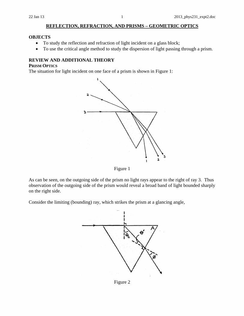
REVIEW AND ADDITIONAL THEORY PRISM OPTICS The situation for light incident on one face of a prism is shown in Figure 1:
Figure 1
As can be seen, on the outgoing side of the prism no light rays appear to the right of ray 3. Thus observation of the outgoing side of the prism would reveal a broad band of light bounded sharply on the right side. Consider the limiting (bounding) ray, which strikes the prism at a glancing angle,
Figure 2

22 Jan 13 2 2013_phys231_expt2.doc
From geometry, (90° – C) + (90° – ) + A = 180° Therefore, A = C + (1) From Snell's law, at the incident face of the prism nair sin 90 = nG sin C 1 = nG sin C (2) and at the outgoing face, nG sin = sin (3) where nair = 1 and nG is nGLASS. From (1), = A – C nG sin = nG sin(A – C) = nG sinA cos C – nG cosA sin C and since nG sin C = 1, nG sin = nG sinA cos C – cosA Substituting into (3): nG sinA cos C – cosA = sin (4) sin2 + cos2 = 1 yields (nG sin C)2 + (nG cos C)2 = nG
2 and from (2), nG sin C = 1,
so nG cos C = nG2 1
(4) becomes sinA nG2 1 – cosA = sin
and 1sin
cossin2
G
A
An
(5)
Therefore, measuring the angle and knowing or measuring the prism angle A enables determination of the index of refraction of the prism glass. As will be observed, the value of nG depends on the wavelength of light incident on the prism. This phenomenon is known as dispersion.

22 Jan 13 3 2013_phys231_expt2.doc
EXPERIMENT REFLECTION AND REFRACTION Place the glass block on top of a piece of paper. Shine the laser on the glass block as shown so that you can see the incident ray, the reflected ray, and the outgoing ray on the far side of the block.
Figure 3
On the paper, carefully trace the location of the glass block, the incident ray, the reflected ray and the outgoing ray. Be sure to mark the location where the light enters the glass block and the location where the light exits the glass block.
DISPERSION OF LIGHT PASSING THROUGH A PRISM Refer to the Spectrometer Adjustment document. It will be assumed that the prism/grating table and telescope and collimator optical axes are properly adjusted, i.e. perpendicular to the central mechanical axis of the spectrometer.
Adjust the spectrometer for parallel rays.
Measure the apex angle, A, of your prism by recording the positions of the reflected ray on the left and the reflected ray on the right. (See Spectrometer Adjustment document.)
Arrange the equipment as shown in Figure 4 below:
glass block
laser

22 Jan 13 4 2013_phys231_expt2.doc
The light shield can consist of a number of layers of masking tape trimmed to exactly cover the unused face of the prism. The collimator is not used and is turned out of the way.
The sodium source will be used to properly orient the equipment. No interference filter will be required for this part of the experiment. Place the ground glass plate between the source and the spectrometer to diffuse the light from the source.
Looking through the telescope, observe the sharp boundary corresponding to the cutoff angle . The sharpness of the cutoff boundary depends on the illumination of the prism. The cutoff boundary should be made as sharp as possible by adjustment of the relative positions of the illumination and the prism face. This is done by rotating the prism table.
Once the critical angle cutoff has been made as sharp as possible, the prism table should be locked, and should not be moved for the remainder of the experiment.
Centre the boundary (cutoff line) in the crosshairs and read the angle. Now move the telescope so that it is perpendicular to the prism face. Unfortunately, this must be done ‘by eye’ and so is not very precise. However, assuming that the objective end of the telescope is perpendicular to the optical axis, placing a steel rule against the end of the telescope should enable the telescope to be positioned to within 0.5° of normal to the prism face.
Figure 5 Record the angle reading when the telescope is normal to the prism face. The cutoff angle is the difference between the reading when the telescope is normal (perpendicular) and the reading when the telescope is centred on the cutoff boundary.
Replace the sodium source with the mercury source. With no filter in place, a series of coloured bands will be seen in the telescope because mercury has several bright emission lines, each with a slightly different critical angle cutoff. As mentioned in the theory, this variation of cutoff angle (and hence refractive index) with wavelength is called dispersion. A set of interference filters is provided to enable determination of the critical angle cutoff for each spectral line.

22 Jan 13 5 2013_phys231_expt2.doc
Measure the cutoff angle readings for the red, yellow, green, blue, and violet mercury spectral lines, in that order.
ANALYSIS REFLECTION AND REFRACTION 1. Calculate the angle of incidence and the angle of reflection. Is the law of reflection verified?
2. Calculate the index of refraction of the glass block. You may assume that the index of refraction of air is 1.00.
DISPERSION OF LIGHT PASSING THROUGH A PRISM 1. Calculate the apex angle of the prism.
2. Calculate the cutoff angles for the Na and Hg spectral lines.
3. Calculate (to 3 decimal places) the refractive index of the prism glass for each of the wavelengths measured.
Tabulate the data and results as follows: A =
Source Colour Wavelength, (nm)
Normal Reading ( __)
Cutoff Reading ( __)
Cutoff Angle ( __)
Refractive Index, n
Na Yellow 589.3 Hg Red 1 623.4
Yellow 578.0 Green 546.1 Blue 3 435.8 Violet 1 404.7
4. Plot refractive index versus wavelength.
5. Now plot refractive index versus inverse wavelength squared. i.e. n vs. 1/2. What does this graph suggest?

10 Feb 12 1 2013_phys231_expt3.doc
SINGLE- AND MULTIPLE-SLIT INTERFERENCE-DIFFRACTION PATTERNS OBJECT
To investigate the diffraction pattern of a single slit, and the interference-diffraction patterns of N-slit rulings for various numbers of slits and various slit widths.
REVIEW OF THEORY SINGLE-SLIT DIFFRACTION There is an intensity maximum in the forward direction, which we shall choose as the reference direction = 0° for angular measurements. The intensity at angle is given by
I I
a
a( )
sinsin
sin
MAX
2
(1)
where is the wavelength of the incident light. The resulting pattern is shown in Figure (1).
Figure (1) There is a strong central maximum, and minima occur when a sin = n for n = 1, 2, 3, ... (2) There are maxima of intensity between the minima, but they fall off rapidly in intensity away from the central maximum. Notice that the central diffraction lobe is twice as wide (in units of
(a sin
)) as the non-central lobes.
10 Feb 12 2 2013_phys231_expt3.doc
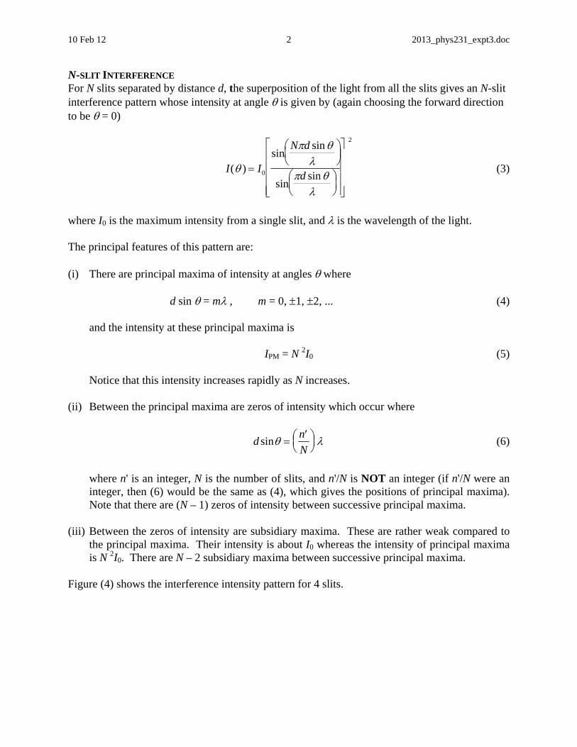
N-SLIT INTERFERENCE For N slits separated by distance d, the superposition of the light from all the slits gives an N-slit interference pattern whose intensity at angle is given by (again choosing the forward direction to be = 0)
I I
N d
d( )
sinsin
sinsin
0
2
(3)
where I0 is the maximum intensity from a single slit, and is the wavelength of the light. The principal features of this pattern are: (i) There are principal maxima of intensity at angles where d sin = m , m = 0, 1, 2, ... (4) and the intensity at these principal maxima is IPM = N 2I0 (5) Notice that this intensity increases rapidly as N increases. (ii) Between the principal maxima are zeros of intensity which occur where
dn
Nsin
(6)
where n' is an integer, N is the number of slits, and n'/N is NOT an integer (if n'/N were an
integer, then (6) would be the same as (4), which gives the positions of principal maxima). Note that there are (N – 1) zeros of intensity between successive principal maxima.
(iii) Between the zeros of intensity are subsidiary maxima. These are rather weak compared to
the principal maxima. Their intensity is about I0 whereas the intensity of principal maxima is N 2I0. There are N – 2 subsidiary maxima between successive principal maxima.
Figure (4) shows the interference intensity pattern for 4 slits.

10 Feb 12 3 2013_phys231_expt3.doc
Figure (4) Notice that there are 4 – 1 = 3 zeros and 4 – 2 = 2 subsidiary maxima between successive principal maxima. N-SLIT INTERFERENCE-DIFFRACTION PATTERNS In the preceding section we considered only the interference between the various slits. However, each slit has its own diffraction pattern. The net observed pattern is the product of the single slit diffraction pattern and the N-slit interference pattern. The combined interference-diffraction pattern is given by the equation
I I
N d
d( )
sinsin
sinsin
0
2
sinsin
sin
a
a
2
(7)
As an example, the combined interference-diffraction pattern for a 3 slit ruling of slit width a and slit separation d = 3a is shown in Figure (5).

10 Feb 12 4 2013_phys231_expt3.doc
Figure (5) When a set of slits (called a ruling or grating) has narrow slits and a small slit separation the single-slit diffraction pattern is rather broad, and not apparent to the observer. The subsidiary maxima are also no longer visible. The observer sees the bright, sharp principal maxima of the N-slit interference pattern. Recall (equation (4)) that the positions of the principal maxima depend on the wavelength of the incident light. Therefore, if the incident light is not monochromatic, the ruling will cause the incident light to be split into its component colours. Thus by knowing the slit separation for a ruling and measuring the angular locations of the principal maxima for a specific colour (called a spectral line) the wavelength of this colour (line) can be determined. m = d sin , m = 0, 1, 2, ... (8) The first principal maximum on one side of the slit image (m = 0) occurs for m = 1, and is said to be the first order maximum. The first order maximum on the other side of the slit image occurs for m = –1. That is, the pattern is symmetric about the incident direction (provided the ruling is mounted perpendicularly to the incident light). Also notice that the possibility exists for a spectral line of one wavelength in one order to be overlapped by a spectral line of another wavelength from a different order. In other words, the angular location for two different colours from different orders could be the same. This would result in the observer seeing a third colour (different from the two component colours) at this location! This ‘new’ spectral line is called an anomalous line since it does not originate from the light source.
10 Feb 12 5 2013_phys231_expt3.doc
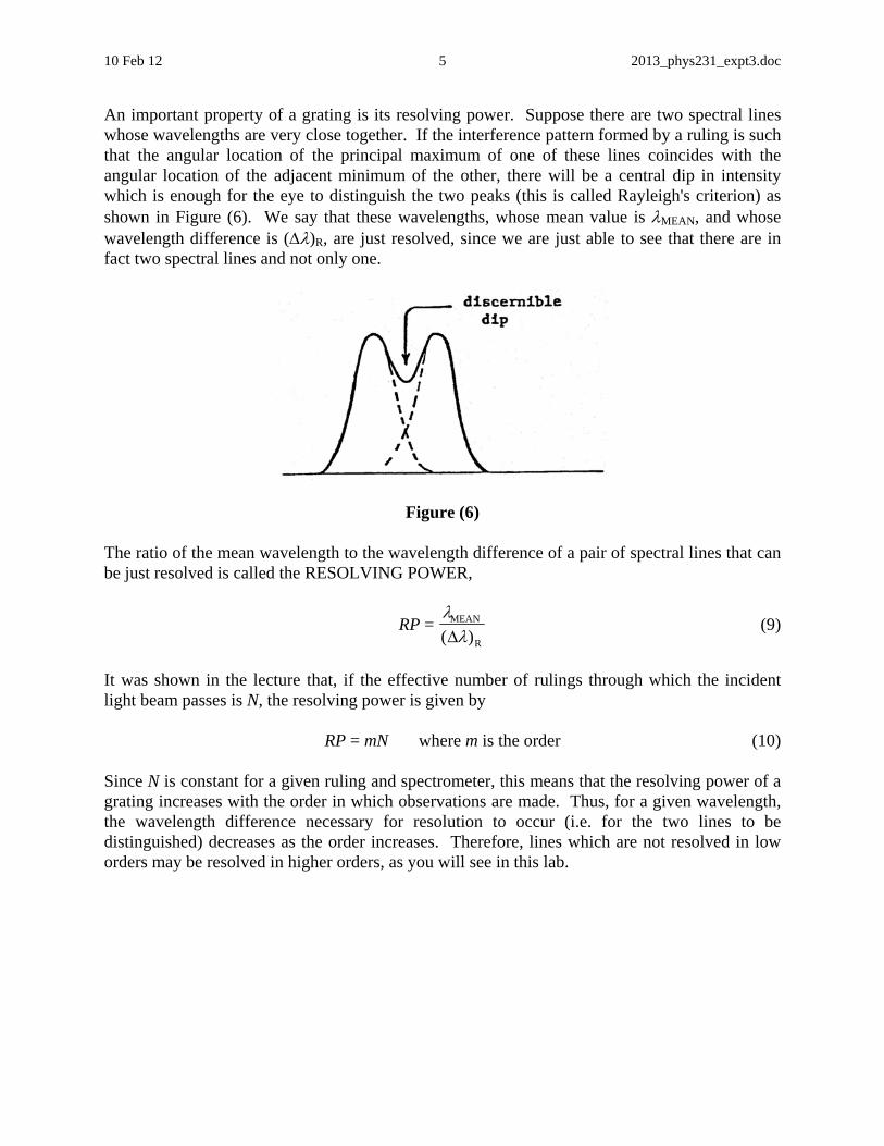
An important property of a grating is its resolving power. Suppose there are two spectral lines whose wavelengths are very close together. If the interference pattern formed by a ruling is such that the angular location of the principal maximum of one of these lines coincides with the angular location of the adjacent minimum of the other, there will be a central dip in intensity which is enough for the eye to distinguish the two peaks (this is called Rayleigh's criterion) as shown in Figure (6). We say that these wavelengths, whose mean value is MEAN, and whose wavelength difference is ()R, are just resolved, since we are just able to see that there are in fact two spectral lines and not only one.
Figure (6) The ratio of the mean wavelength to the wavelength difference of a pair of spectral lines that can be just resolved is called the RESOLVING POWER,
RP =
MEAN
R( ) (9)
It was shown in the lecture that, if the effective number of rulings through which the incident light beam passes is N, the resolving power is given by RP = mN where m is the order (10) Since N is constant for a given ruling and spectrometer, this means that the resolving power of a grating increases with the order in which observations are made. Thus, for a given wavelength, the wavelength difference necessary for resolution to occur (i.e. for the two lines to be distinguished) decreases as the order increases. Therefore, lines which are not resolved in low orders may be resolved in higher orders, as you will see in this lab.
10 Feb 12 6 2013_phys231_expt3.doc
EXPERIMENT 1. Plug in the mercury source. Adjust the telescope and collimator of the spectrometer for
parallel light as described in the spectrometer adjustment documentation. Mount the 546 nm filter on the collimator end of the spectrometer. This allows only the green line at 546.074 nm to pass.
2. You are given a slide containing rulings with 1 to 6 slits. Each ruling has the same slit
width a and slit separation d.
(i) Examine the single-slit pattern. In order to obtain an easily visible pattern, you may have to open the collimator slit. In your lab notebook, draw a sketch of the intensity versus angle (incident direction = 0) for the pattern. Qualitatively compare your observations with the predictions of theory.
(ii) Measure the angular positions of the first and second minima of the single-slit pattern.
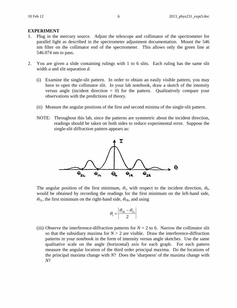
NOTE: Throughout this lab, since the patterns are symmetric about the incident direction,
readings should be taken on both sides to reduce experimental error. Suppose the single-slit diffraction pattern appears as:
The angular position of the first minimum, 1, with respect to the incident direction, 0, would be obtained by recording the readings for the first minimum on the left-hand side, 1L, the first minimum on the right-hand side, 1R, and using
11 1
2
R L
(iii) Observe the interference-diffraction patterns for N = 2 to 6. Narrow the collimator slit
so that the subsidiary maxima for N > 2 are visible. Draw the interference-diffraction patterns in your notebook in the form of intensity versus angle sketches. Use the same qualitative scale on the angle (horizontal) axis for each graph. For each pattern measure the angular location of the third order principal maxima. Do the locations of the principal maxima change with N? Does the 'sharpness' of the maxima change with N?
10 Feb 12 7 2013_phys231_expt3.doc
3. Replace the 1- to 6-slit slide with the Ronchi ruling. A Ronchi ruling is simply a glass plate with black rulings baked on, the width of the rulings and spacings between the rulings being equal. With the Ronchi ruling, the subsidiary maxima are no longer visible and the diffraction pattern is so broad as to not be apparent.
(i) Measuring the angular position of the mercury green line in 5th, 10th, and 15th order. (ii) Replace the 546 nm interference filter with the 577 nm filter. This filter allows only
the yellow pair of spectral lines of mercury to pass. Observe that in low orders the yellow pair appears to be a single line, but that in higher orders it is observable that in fact there are two closely-spaced lines. Measure the angular position of the yellow pair in a known (high) order.
(iii) Adjust the collimator slit so that the lines are as sharp as possible but still visible.
Judge in what order the two lines of the yellow pair are just resolved (i.e. what is the lowest order in which you can tell that there are in fact two lines and not just one).
(vi) In terms of d, calculate the angular position of the 3rd order yellow pair (use =
578.0 nm) and the angular position of the 4th order blue 3 line.
i.e. dd
d YYYY
nm 1734arcsin
3arcsin3sin
, and similarly for B.
Open the collimator slit slightly so that the lines are easily visible, yet not too wide. Position the cross hair of the telescope on the 3rd order yellow pair. Now without moving the telescope replace the 577 nm filter with the 435 nm filter. This filter passes only the blue mercury lines. What do you observe? Is the cross hair on one of the blue lines? If so, which order? Finally, remove the filter and observe the unfiltered mercury spectrum. What colour is the spectral line on which the cross hair is located? This unexpected spectral colour is called an anomalous line, since it arises not from the atomic energy levels of the source, but from the nearly geometric ratio of the wavelengths of at least two spectral lines of the source.
(vii) In terms of d, calculate the angular position of the 4th order green line and the angular
position of the 5th order blue line. Insert the 546 nm (green) filter. Position the cross hair on the 4th order green line. Without moving the telescope replace the 546 nm filter with the 435 nm (blue) filter. Is the cross hair on one of the blue lines? If so, which order? Remove the filter and observe the unfiltered mercury spectrum. What colour is the spectral line on which the cross hair is located? This unexpected spectral colour is another anomalous line.

10 Feb 12 8 2013_phys231_expt3.doc
Accepted Values of Mercury Spectrum
Colour Wavelength
(nm) Relative Intensity
Violet 1 404.7 10 Violet 2 407.8 7 Blue 1 433.9 5 Blue 2 434.8 5 Blue 3 435.8 10 Blue Green 1 491.6 7 Blue Green 2 496.0 6 Green 546.1 10 Green Yellow 567.6 4 Yellow 1 577.0 10 Yellow 2 579.1 10 Orange 1 607.3 5 Orange 2 612.3 5 Red 1 623.4 7 Red 2 690.7 4
ANALYSIS 1. Using the measurements from 2. (ii), calculate an average value for the slit width a.
2. Using the measurements from 2. (iii) of the principal maxima for N = 6, calculate the slit separation d.
3. Using the measurements from 3. (i) in dm
sin
, calculate d for each of the 3 sets of
measurements and calculate the average.
4. Using the measurements from 3. (ii), calculate the average wavelength for the yellow pair.
5. Using the average wavelength for the yellow pair and the wavelength difference calculated from the wavelength table, calculate the resolving power when the yellow pair is just resolved (equation 9).
6. Using the value obtained in 3. (iii) for the just-resolved order and the resolving power calculated above, calculate the effective number of rulings across the width of the collimated beam (use equation 10).

8 Mar 12 1 2013_phys231_expt4.doc
MICROWAVE OPTICS AND POLARISATION OBJECTS
To investigate whether microwaves obey the law of reflection; To use a Michelson interferometer to measure the microwave wavelength; To investigate double slit interference of microwaves; To investigate polarisation of microwaves.
REVIEW OF THEORY DOUBLE-SLIT INTERFERENCE For two slits of width a separated by distance d, the superposition of the waves from the slits gives an interference-diffraction pattern whose intensity at angle is given by (choosing the forward direction to be = 0):
2
0 sinsin
sin2sin
)(
d
d
II
2
sin
sinsin
a
a
2
0 sinsin
sin2cos
sin2sin2
)(
d
dd
II
2
sin
sinsin
a
a
sin2
cos4)( 20
dII
2
sin
sinsin
a
a
where I0 is the maximum intensity from a single slit, and is the wavelength. The principal features of this pattern are: (i) There are maxima of intensity at angles where
d sin = m , m = 0, 1, 2 ... (ii) There are minima (zeros) of intensity at angles where
d sin = (m + ½) , m = 0, 1, 2 ... (iii) Diffraction results in the overall intensity decreasing as increases.

8 Mar 12 2 2013_phys231_expt4.doc
The following figure shows the overall intensity pattern:
EXPERIMENT MICROWAVE OPERATING INSTRUCTIONS 1. Keep the Variable Sensitivity control turned fully counter-clockwise (minimum setting).
2. Turn the Receiver OFF when not in use. (It is battery powered.)
3. Do not place your hand or any other object within the field while making measurements – this causes inaccurate Microammeter readings.
4. The Microammeter is damped to reduce the effect of variation in the input line voltage. Thus when seeking a peak reading by moving either the Transmitter, Receiver, Rotary Platform, or Sliding Accessory Holder, all changes in position should be made slowly.
5. The receiver reading is obtained by multiplying the meter reading by the scale factor. i.e. 30 is the LEAST sensitive scale and 1 is the MOST sensitive scale.

8 Mar 12 3 2013_phys231_expt4.doc
MEASUREMENT OF REFLECTION Arrange the equipment as shown:
Record the angular position of the Transmitter, T. Position the Reflector at an angle to the microwave beam from the Transmitter (thus defining an angle of incidence i) and record the angular position of the right edge (as seen from above) of the Reflector, Rf. Slowly rotate the Receiver about the central axis until a peak reading is obtained on the Microammeter. Record this angular position of the Receiver, R. Repeat the above measurements for two other incident angles. MICHELSON INTERFEROMETER Arrange the equipment as shown:
Position the Moveable Reflector A close to the Half-Reflector C.

8 Mar 12 4 2013_phys231_expt4.doc
Slowly slide the Moveable Reflector away from the Half-Reflector until a maximum reading is obtained on the Microammeter. Record the position of the Moveable Reflector. Continue to slide the Moveable Reflector away from the Half-Reflector, recording the positions of the Moveable Reflector for at least 10 consecutive maxima. DOUBLE SLIT INTERFERENCE Assemble the double-slit by using the two wide and one narrow metal plates and the slit extender arm, as shown:
Set the slit width to be about 1.5 cm. Measure the centreline slit separation, d. Place the Transmitter horn about 5 cm from the slits. Position the Receiver at 90° to the Transmitter. Slowly move the Receiver through 180°, taking readings from the Microammeter every 5°. POLARISATION Arrange the equipment as shown:
Ensure that the rotational positions of both the transmitter and receiver are 0, so that their polarisation axes are vertical. Adjust the Receiver settings for approximately full-scale meter
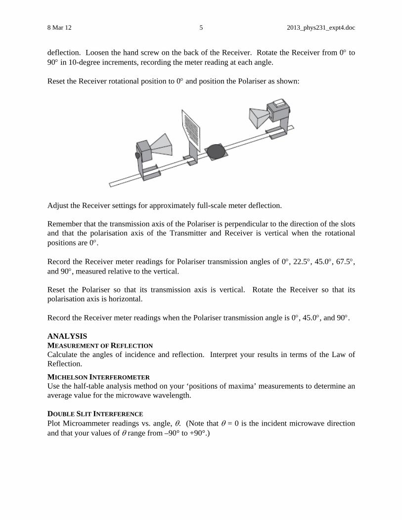
8 Mar 12 5 2013_phys231_expt4.doc
deflection. Loosen the hand screw on the back of the Receiver. Rotate the Receiver from 0 to 90 in 10-degree increments, recording the meter reading at each angle. Reset the Receiver rotational position to 0 and position the Polariser as shown:
Adjust the Receiver settings for approximately full-scale meter deflection. Remember that the transmission axis of the Polariser is perpendicular to the direction of the slots and that the polarisation axis of the Transmitter and Receiver is vertical when the rotational positions are 0. Record the Receiver meter readings for Polariser transmission angles of 0, 22.5, 45.0, 67.5, and 90, measured relative to the vertical. Reset the Polariser so that its transmission axis is vertical. Rotate the Receiver so that its polarisation axis is horizontal. Record the Receiver meter readings when the Polariser transmission angle is 0, 45.0, and 90. ANALYSIS MEASUREMENT OF REFLECTION Calculate the angles of incidence and reflection. Interpret your results in terms of the Law of Reflection.
MICHELSON INTERFEROMETER Use the half-table analysis method on your ‘positions of maxima’ measurements to determine an average value for the microwave wavelength. DOUBLE SLIT INTERFERENCE Plot Microammeter readings vs. angle, . (Note that = 0 is the incident microwave direction and that your values of range from –90° to +90°.)
8 Mar 12 6 2013_phys231_expt4.doc
Compare the experimental maxima angles obtained from your graph with the theoretical angles obtained from = arcsin(m/d) (use the value of wavelength determined from the Michelson Interferometer analysis). Discuss. POLARISATION Plot Receiver meter reading vs. Receiver rotation angle. Discuss and explain the shape of the graph. Plot Receiver meter reading vs. angle of the Polarisation transmission axis with respect to the vertical. Discuss and explain the shape of the graph. Discuss and explain the results obtained when the Transmitter and Receiver were perpendicular and the orientation of the Polariser was varied.
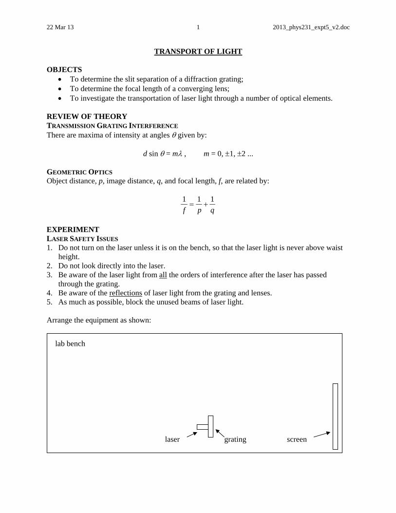
22 Mar 13 1 2013_phys231_expt5_v2.doc
TRANSPORT OF LIGHT OBJECTS
To determine the slit separation of a diffraction grating; To determine the focal length of a converging lens; To investigate the transportation of laser light through a number of optical elements.
REVIEW OF THEORY TRANSMISSION GRATING INTERFERENCE There are maxima of intensity at angles given by:
d sin = m , m = 0, 1, 2 ... GEOMETRIC OPTICS Object distance, p, image distance, q, and focal length, f, are related by:
qpf
111
EXPERIMENT LASER SAFETY ISSUES 1. Do not turn on the laser unless it is on the bench, so that the laser light is never above waist
height. 2. Do not look directly into the laser. 3. Be aware of the laser light from all the orders of interference after the laser has passed
through the grating. 4. Be aware of the reflections of laser light from the grating and lenses. 5. As much as possible, block the unused beams of laser light. Arrange the equipment as shown:
laser grating screen
lab bench
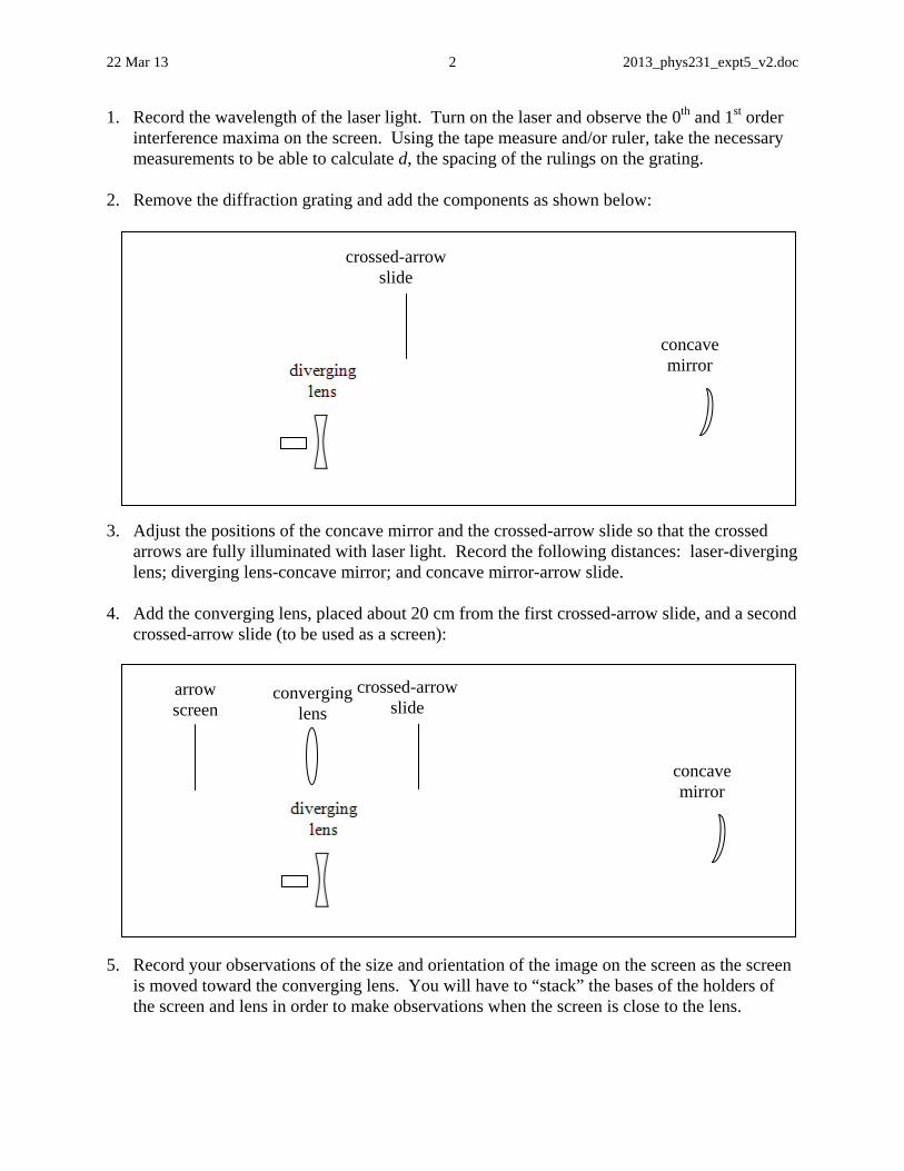
22 Mar 13 2 2013_phys231_expt5_v2.doc
1. Record the wavelength of the laser light. Turn on the laser and observe the 0th and 1st order interference maxima on the screen. Using the tape measure and/or ruler, take the necessary measurements to be able to calculate d, the spacing of the rulings on the grating.
2. Remove the diffraction grating and add the components as shown below: 3. Adjust the positions of the concave mirror and the crossed-arrow slide so that the crossed
arrows are fully illuminated with laser light. Record the following distances: laser-diverging lens; diverging lens-concave mirror; and concave mirror-arrow slide.
4. Add the converging lens, placed about 20 cm from the first crossed-arrow slide, and a second
crossed-arrow slide (to be used as a screen): 5. Record your observations of the size and orientation of the image on the screen as the screen
is moved toward the converging lens. You will have to “stack” the bases of the holders of the screen and lens in order to make observations when the screen is close to the lens.
concave mirror
crossed-arrow slide
converging lens
crossed-arrow screen
concave mirror
crossed-arrow slide
converging lens
arrow screen
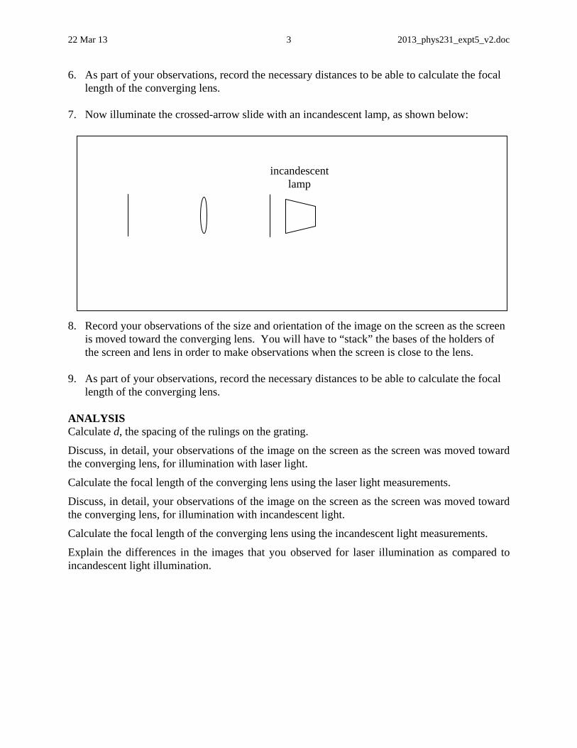
22 Mar 13 3 2013_phys231_expt5_v2.doc
6. As part of your observations, record the necessary distances to be able to calculate the focal length of the converging lens.
7. Now illuminate the crossed-arrow slide with an incandescent lamp, as shown below: 8. Record your observations of the size and orientation of the image on the screen as the screen
is moved toward the converging lens. You will have to “stack” the bases of the holders of the screen and lens in order to make observations when the screen is close to the lens.
9. As part of your observations, record the necessary distances to be able to calculate the focal
length of the converging lens. ANALYSIS Calculate d, the spacing of the rulings on the grating.
Discuss, in detail, your observations of the image on the screen as the screen was moved toward the converging lens, for illumination with laser light.
Calculate the focal length of the converging lens using the laser light measurements.
Discuss, in detail, your observations of the image on the screen as the screen was moved toward the converging lens, for illumination with incandescent light.
Calculate the focal length of the converging lens using the incandescent light measurements.
Explain the differences in the images that you observed for laser illumination as compared to incandescent light illumination.
converging lens
crossed-arrow screen
incandescent lamp