A Java planner for Blocksworld problems

A Bachelor’s thesis

15220 words

by Elif Aktolga

elif81@web.de 19th January 2004

Supervisors: PD. Dr. rer. nat. Ute Schmid

Dr. habil. Helmar Gust

University of Osnabrueck WS 03/04

2

Abstract

Intelligent strategies are indispensable for solving problems arising daily in life. Knowledge-based intelligent strategies are required to solve such problems efficiently and to obtain the desired result. This is e.g. achieved by finding a sequence of actions that lead from the initial state to the goal state. We refer to this as planning. In Cognitive Science, human problem solving and planning is analysed; in Artificial Intelligence this behaviour is attempted to be simulated in machines – with varying methods. This paper overviews current planning approaches and deals with the core parts of problem solving and (linear-) total-order state-based planning. Additionally, this work is based on a non-linear Java planner that implements the essential parts mentioned above using the Blocksworld domain and Blocksworld problems.

Zusammenfassung

Intelligente Strategien sind unentbehrlich beim Lösen von Problemen, die einem im täglichen Leben begegnen. Wissensbasierte intelligente Strategien sind erforderlich, um Probleme effizient zu lösen und das erwünschte Resultat zu erhalten. Dazu muss man z.B. eine Folge von Zuständen finden, die vom Startzustand zum gewünschten Endzustand führt. Dies nennt man Planen. In Cognitive Science wird menschliches Problemlösen und Planen analysiert; in der Künstlichen Intelligenz wird versucht dieses Verhalten mit verschiedenen Methoden in Maschinen zu simulieren. Diese Arbeit verschafft einen Überblick über aktuelle Planungsmethoden und -systeme; der Hauptteil der Arbeit befasst sich ausschließlich mit klassischem Problemlösen und dem (linearen) Zustands-Basierten Planen, in der die Abfolge der Operatoren vollständig determiniert ist. Außerdem stützt sich die Arbeit auf einen nicht-linearen Java-Planer, in dem die o. g. Konzepte implementiert sind. Als Anwendungsbeispiel werden die Blockswelt-Domäne und Blockswelt-Probleme verwendet.

3

Table of Contents

1 Introduction.............................................................................................. 5 1.1 Motivation.......................................................................................................................5 1.2 What do Problem Solving and Planning involve?......................................................5 1.3 Problem Solving and Planning.....................................................................................6

1.3.1 The Cognitive Approach........................................................................................6 1.3.2 The Computational Approach..............................................................................7

1.4 Classical Planning and Production Systems..............................................................7 1.4.1 Linear Strategy and Total-Order Planning .........................................................7 1.4.2 Non-linear Strategy and Partial-Order Planning...............................................8 1.4.3 State-Space and Plan-Space Planning ................................................................8 1.4.4 Hierarchical Planning.............................................................................................9

1.5 About the scope of this work and the underlying implementation......................9

2 Problem Solving and Planning ..............................................................10

2.1 Basic Formalism and Definitions ..............................................................................10 2.1.1 STRIPS.....................................................................................................................10 2.1.2 PDDL.......................................................................................................................11 2.1.3 The Blocksworld Domain ....................................................................................11 2.1.4 Predicate ................................................................................................................11 2.1.5 State........................................................................................................................12 2.1.6 Operator/Action...................................................................................................13 2.1.7 Operator-State Pair..............................................................................................15 2.1.8 Search Tree............................................................................................................15

2.2 Classical Search...........................................................................................................16 2.2.1 Uninformed Search Algorithms..........................................................................16

2.2.1.1 Breadth-First Search.....................................................................................17 2.2.1.2 Depth-First Search........................................................................................17

2.2.2 Informed Search Algorithms...............................................................................18 2.2.2.1 Greedy Search................................................................................................19 2.2.2.2 A* Search........................................................................................................20

2.3 State-Based Planning..................................................................................................21 2.3.1 Planning Problem.................................................................................................21 2.3.2 Operator Application...........................................................................................22

2.3.2.1 Forward Operator Application.....................................................................22 2.3.2.2 Backward Operator Application..................................................................23

2.3.3 Generation of successor states..........................................................................23 2.3.4 Main planning algorithm.....................................................................................25 2.3.5 Some Blocksworld Problems...............................................................................27 2.3.6 Blocksworld Heuristics for Informed Search....................................................27

4

3 Implementation of the planner .............................................................30 3.1 Overview of Classes....................................................................................................30 3.2 Parsing PDDL to Java...................................................................................................32

3.2.1 Lexical Analyser....................................................................................................32 3.2.2 Syntax Analyser....................................................................................................33 3.2.3 Code Generation...................................................................................................34 3.2.4 Detection of errors...............................................................................................34

3.3 The Applet....................................................................................................................34 3.3.1 Illustration.............................................................................................................35 3.3.2 Output of the Planner..........................................................................................36

4 Conclusion..............................................................................................38

4.1 Achievements and Problems.....................................................................................38 4.2 Outlook.........................................................................................................................38

References .................................................................................................39

Appendix ...................................................................................................41

Extension to part 3.2.2 (Syntax Analyser)..................................................................41 Blocksworld domain file ................................................................................................41 Blocksworld problem files.............................................................................................42

5

1 Introduction This chapter introduces and motivates the field of problem solving and planning. It is based on the cognitive and historical basis of the two fields, however differences between the psychological and computational approach are revealed. A historical overview of the most important planning systems is given in section 1.4. The connection between this chapter and the underlying Java implementation is discussed in the last part of this chapter.

1.1 Motivation Problem solving and planning are relevant to Artificial Intelligence. Particularly in the fields of game playing, robots utilise problem solving and planning techniques to accomplish their tasks. However, problem solving and planning are also required in every day situations, where human beings are confronted with problems and must construct plans to solve them. The aim of this thesis is to demonstrate the methods applied by human beings and in AI for problem solving and planning. Within AI, problem solving and planning are utilised for situations where complex strategic and reasoned behaviour is required. Two aspects are significant: Knowledge about the problem and the applied strategy. Characteristic languages for AI are Prolog, LISP, or ML, since these logical and functional programming languages facilitate knowledge representation and rule application. Matching is an important issue, i.e. substituting and mapping variables with concrete terms. Another programming concept that is used extensively nowadays – though not in AI – is object-oriented programming. Java is a relatively new example of this paradigm that has proven to be very flexible. The aim of the programming part of this work was to use an untypical AI programming language like Java to implement a simple non-linear and total-order planner. Blocksworld, which is a well-known planning example, is used as a domain for testing. Chapter 1 introduces the fields from a cognitive and computational point of view. Current approaches to planning are discussed briefly. Chapter 2 then explains the basic concepts of problem solving and planning with reference to the implementation. Chapter 3 describes the non-planning parts of the implementation like parsing and illustration of the applet. Chapter 4 concludes from the overall work.

1.2 What do Problem Solving and Planning involve? Problem solving and planning are two core fields of AI. Problem solving comprises standard search problems. Planning is typically viewed as a generic term of problem solving because it deals with search on an abstract level. Problem solving is typically more concerned with plan execution, whereas planning is involved with plan generation. This is due to the fact that problem solving systems are usually designed to solve one specific task and therefore they are restricted. However, modern planning systems are able to deal with much harder problems and unexpected issues that arise during the planning process. Since the scope of problems dealt with in planning is much wider, a planner is viewed as the producer or generator of the solution, and a problem solving system just “demonstrates” one specific solution. Cognitive science typically deals with information processing: “The human mind is viewed as a complex system that receives, stores, retrieves, transforms, and transmits information. These operations on information are called computations or information processes.” […] (qt. from Stillings et al., 1998). In AI, machines or computers are designed to perform these computations, though not necessarily in a “human way” as described above. This is due to the fact that artificial intelligent systems do not possess goal-determining organisms.

6

Within the scope of cognitive science, a planner that comprises planning and problem solving techniques can be considered as an information processing system. The task of this system is to receive information as input – a search or planning problem – and to produce an output that represents the solution path to this problem. Two examples shall be discussed from the real world. Imagine, one wants to build a house. What has to be done? One has to consult an architect, who will construct a plan that will ideally include all the wishes and ideas that one has in mind about the house. The architect will hand over the theoretical plan on paper to a civic engineer. This person will execute the plan by means of construction workers (“motor systems”) according to the prescriptions of the architect, but he or she will also contribute his own knowledge to the plan, e.g. about which material to choose, how it shall be processed etc. If we regard this problem “building a house” from an AI point of view, then the architect and civic engineer form the information processing system. The architect performs the plan generation on a more abstract level – the planning, and the civic engineer executes this plan and applies his problem-specific knowledge to it – he does the problem solving. The second example is a characteristic cognitive science one: Human problem solving or thinking. If one reflects on a specific problem that must be solved, one constructs a plan in the prefrontal cortex. This plan is passed on to the cerebellum and the basal ganglia and it is prepared for execution. Once the plan is ready to be executed, it is passed on to the motor system for physical execution. Typically, in this example plan generation is done in the brain, whereas plan execution is performed physically by the motor system visibly to the outer world. In planning, hard problems are approached by problem decomposition. If a problem is too difficult to solve as a whole, it is divided into small tasks with subgoals. Consequently, these have to be solved by the planner. Once all subgoals are solved, the solution is synthesised. Planning uses knowledge representation schemes such as STRIPS, situation calculus, PDDL etc. to represent planning problems (Marshall, 1996).

1.3 Problem Solving and Planning In cognitive psychology human problem solving is an area of research, rather than planning. In AI both play an important role, which has been described in the previous section. In this part, the relevant features of both shall be discussed and highlighted. This section is largely based on (Schmid, 2002), (Schmid, 2003), and (Stillings et al., 1998).

1.3.1 The Cognitive Approach In cognitive psychology theories and models of human information processing are proposed and tested empirically. Human problem solving and reasoning are typical, overlapping fields. Still, the term “reasoning” is rather used to refer to drawing inferences, whereas problem solving refers to performing domain-specific tasks. Newell and Simon studied human problem solving in the early 1960’s and developed the GPS (General Problem Solver) in 1972. The GPS uses means-ends analysis and subgoaling (problem decomposition) for simulation of human problem solving. As a result of their research, they hypothesised that human beings solve problems within a problem space, which contains all the possible situations or cases of the problem (states), and operators that lead from one state to another (state transformation). In order to solve a problem, one has to find a solution path from the initial state to the goal state (desired state) by applying operators. Means-ends analysis is a typical human strategy for operator selection: The operator is chosen that most reduces the remaining difference between the current state and the goal state. This is accomplished with a difference operator table (Schmidt, 1996). Still, this technique is not a very good one, since an operator that looks promising to solve the

7

problem might also be misleading. Additionally, problem-specific knowledge about each state is required. A production system in cognitive psychology is fairly analogous to a planning system in AI. It resembles the cognitive architecture of human beings in that it can hold facts (declarative knowledge stored in a database) about the to-be-solved problem and rules (procedural knowledge). It applies these rules or definitions to the problem by using an interpreter. The interpreter goes through match-select-apply cycles during rule application, i.e. it matches the available rules with the current state, selects a suitable rule according to a strategy (e.g. means-ends analysis), and applies this to the state to obtain the successor state (note the parallels between this system and planning systems in Chapter 2). Rules typically consist of if-then clauses as used in programming languages in computer science. Human beings typically think and act in a goal-driven way (Stillings et al., 1998). Therefore, their problem solving is guided by goals. Although the human brain is able to solve complex problems in every day situations, due to memory and time limitations, mostly simpler strategies are preferred over complicated ones. Still, as human beings possess the skill of thinking creatively, including their experience and logic, they are superior to computers and machines in many fields of problem solving. So far in game playing, particularly chess, computational performance is somewhat comparable with human cognition.

1.3.2 The Computational Approach In AI, we talk about planning systems within the fields of problem solving and planning. These are typically efficient computer programs, or “formalised information processes” (qt. from Schmid, 2002). Consistency is important, i.e. the program – representing a system – must return stable outputs to all possible inputs. This also contributes to the efficiency of the program. Computers store, maintain, and process information differently than human beings do. So the aim of AI is not to build computer systems that process information exactly like human beings do. Still, human problem solving is an example for AI and therefore it is not surprising to find many parallels between the areas. Characteristic of planning systems are the usage of states, operators (correspond to rules in production systems), search algorithms and heuristics (strategy), as well as domain-specific knowledge (see Chapter 2). Basically, the roots of the computational and cognitive approach are the same, starting with Newell and Simon’s GPS. However, as more complex planning problems have been examined, different planning concepts arose that are briefly discussed in the next section. It is particularly interesting to observe that the tendency of modern planning systems goes towards abstraction and generalisation of problems. Therefore, nowadays a good planner should be applicable to many domains, being able to deal with arising problems; it should be able to backtrack and solve goals parallel and not sequentially.

1.4 Classical Planning and Production Systems In this section the best-known classical planning and production systems of the past 30-40 years will be outlined. The content of this part is largely based on (Russel & Norvig, 2003) and (Schmid, 2003).

1.4.1 Linear Strategy and Total-Order Planning STRIPS was the first significant linear planning system introduced by Fikes and Nilsson in 1971. It is used and described later on especially in Chapter 2 (see section 2.1.1). STRIPS uses concepts of GPS as introduced earlier and of the QA3 proving system by Green in

8

1969. Characteristic of all these planning systems is their linear approach, i.e. only one aim is followed and attempted to be solved – interleaving of goals is not allowed. So, goals are maintained on a stack and dealt with one by one. Additionally, only totally ordered action sequences are allowed, i.e. the order of actions cannot be changed later on and must be strictly determined once planning is complete (total-order planning). Soon after the invention of STRIPS, which actually represents both a language for planning systems and the system itself, the languages ADL (Action Description Language) by Pednault (1986), and PDDL (Planning Domain Definition Language) by Ghallab et. al. (1998) followed. PDDL is the language that is used for my underlying Java planning system (please refer to section 2.1.2). As to problem solving, A*, which was introduced by Hart, Nilsson, and Raphael in 1968, is worth mentioning since it is also utilised in many planning systems. A* is the current best-performing search algorithm. It has been changed and varied after its emergence in 1968. For more detail please refer to section 2.2.2.2.

1.4.2 Non-linear Strategy and Partial-Order Planning Soon after the linear strategy of planning was proposed, it became evident that it was incomplete: It was insufficient for interaction of goals (Simmons, 2001). The so-called Sussman anomaly, discovered by Brown in 1975, proved that interleaving of goals is required to solve specific problems. As mentioned before, problem decomposition is typically applied in planning systems. The Sussman anomaly showed that some subgoals depend on other subgoals, therefore a planning system had to be able to recognise this and switch to the goal that had to be solved first. Thus, the concept of non-linear planning arose and the serialisation of subgoals became standard. Goals were not ordered on a stack any more, instead they were used as a set (Simmons, 2001). NOAH, proposed by Sacerdoti in 1975, was the first planning system that used this approach. Consequently with non-linear planning, the notion of partial-order planning was proposed, too. GRAPHPLAN, invented by Blum and Furst in 1997, uses this idea, as well as IPP (by Koehler et. al., 1997), and STAN (by Fox and Long, 1998). In partial-order planning, the order of actions need not to be fully determined, i.e. if at a specific choice point several solutions are possible, then this choice point is left “open”. Such plans are completed with “plan-space” search (see next section). Partial-order planning also uses a so-called ”least commitment strategy” because only the necessary planning steps and initialisations are accomplished and the redundant ones are omitted as long as possible. This technique was used until the late 1990’s. The development of planning systems clearly progressed towards solving more complex and abstract problems on a higher level.

1.4.3 State-Space and Plan-Space Planning GPS, HSP (Heuristic Search Planner) by Bonet and Geffner in 1999, which generates heuristic functions to given problems, and FASTFORWARD (from Hoffmann in 2000), use the approach of state-space planning. State-space planning refers to the basic approach of search where states are expanded from the initial state to the goal state to find a solution path. The majority of the early days’ and today’s basic planners use this strategy. In plan-space planning, search is performed in a space of plans. Therefore it can be associated with partial-order planning, since it is typically applied to partially finished plans. Remember that partial-order planning allows incomplete plans with open choice points, so these types of plans can be fully ordered in plan space only. NOAH (introduced in the last section), and UCPOP, originally by Weld and Penberthy in 1992, are typical examples for plan-space planners. Production systems, introduced in section 1.3.1, are applied in various fields, such as mathematics, logic, games etc. Typically, state-space search is utilised for these systems.

9

ACT (Adaptive Character of Thought) is one of those systems that should be mentioned: This goal-directed system was introduced by Anderson in 1983. It uses declarative and procedural knowledge for e.g. analogous problem solving. SOAR (State, Operator And Result), proposed by Laird et. al. in 1987, works similarly to ACT and is modelled on GPS.

1.4.4 Hierarchical Planning Hierarchical planning is another planning systems concept. Plan construction is performed on different levels of abstraction, and it resembles some type of abstract problem decomposition. The aim is to reduce problem-specific search by solving a more general version of the problem (Knoblock, 1993). ABSTRIPS, proposed by Sacerdoti in 1974, was the first planner to use this method. HSP, introduced in the previous section, is also a typical example. It uses forward planning (see section 2.3.2.1) to find heuristic functions.

1.5 About the scope of this work and the underlying implementation This thesis refers to the programming work that comes on the CD. The program is a non-linear, total-order, state-based planner written in Java. It has been tested with Blocksworld problems only (see Appendix), but theoretically it is applicable to any kind of problem that can be solved with a total-order and non-linear planning strategy. Domain and problem files have to be specified in PDDL. Please refer to Chapter 3 for the Java implementation. The following second chapter is meant to be the formal basis of the implementation; any definitions mentioned abstractly describe the methods and data types that were used. Therefore only the topics that are relevant for the implementation are specified in the second chapter. Thus, this paper does not discuss further any of the introduced areas of modern planning such as partial-order planning, hierarchical decomposition etc., since this goes beyond the scope of the Java implementation.

10

2 Problem Solving and Planning Problem solving and planning are two related fields of Artificial Intelligence that share many methods. However there are important differences. Planning includes problem solving and deals with more complex problems (Schmid, 2002). Their goals are the same, but the approaches are different. Whereas problem solving is mainly concerned with classical search, i.e. uninformed and informed search algorithms, planning is more general. Detailed and explicit domain and problem-specific knowledge is available in an independent logical format (Schmid, 2003). As a result, planning algorithms and information about the problem are clearly separated. In search the input is mostly optimised and simplified for a specific problem. Predominantly, algorithms and the problem are programmed together, so that they are not compatible with other systems. In contrast, my Java Blocksworld planner could also be used for other domains. Once the source information is available about the operators, domain objects, costs etc. and if at least one problem file is specified, then the planner can easily be applied. This is due to the generalised and flexible planning concept that does not change for different problems. In problem solving, one usually has to alter the whole program if one wants to apply it to a different problem. Planning requires a detailed organisation of advanced and flexible search. It offers many options, such as operator application direction. Backwards planning is typical for planning, whereas in problem solving usually only forward search is utilised. In my Java implementation, both techniques are available. Another difference between problem solving and planning is the usage of operators or “successor functions”. In planning operators can be seen as concrete methods, whereas in common search usually a single successor function is used that is optimised for the problem. This issue is explained in section 2.1.6. This chapter discusses typical topics of the fields problem solving and planning. The first part introduces definitions and the formal issues that are required as base knowledge for this chapter. The second part deals with problem solving only, i.e. the common search strategies. The third part then focuses on state-based planning techniques and extends the first part of this chapter.

2.1 Basic Formalism and Definitions As the two fields problem solving and planning share many components, it is difficult to differentiate between them and to deal separately with both. Since the emphasis is on planning, all the definitions and explanations in this section refer to a planning environment. Still, as some terms typically belong to problem solving (like “state space” in section 2.1.8), the explanations are purposely adjusted only so that they fit the planning concept.

2.1.1 STRIPS The STRIPS language (“Stanford Research Institute Problem Solver”) by (Fikes & Nilsson, 1971), is commonly used in planning for representing states, goals, and actions (Schmid, 2003). The Closed World Assumption (CWA) holds, i.e. any states or relations that are not explicitly defined are assumed to be false. States and goals are represented as conjunctions of positive literals. Operators are used as instantiated actions to transform states to others. STRIPS is like the Situation Calculus, introduced by McCarthy in 1963, but it is much more restricted so that it meets the requirements of a representation language for planning problems. The following definitions in sections 2.1.4 to 2.1.7 about states, predicates, operators, and operator-state pairs are based on the STRIPS language. A formal description of STRIPS can be found in (Schmid, 2003).

11

2.1.2 PDDL PDDL (“Planning Domain Definition Language”) by (McDermott, 1998), is a useful language for representing planning domains and problems. Planning domains build the source knowledge of the planner by providing general information about an environment, defining valid objects, operators, predicates etc. A planning problem specifies some problem to be solved by the planner. Typical components are declarations of the initial and goal state, the used objects, heuristic function, and the domain that is used in conjunction. An example of a planning domain, the Blocksworld domain, and planning problems can be found in the Appendix. PDDL is mainly inspired by STRIPS, but also by many other languages and extensions that arose since the invention of STRIPS. A description of the syntax of PDDL is given in (AIPS-98 Planning Competition Committee, 1998) and also in (Fox and Long, 2003), which is the most recent extension to PDDL. Section 3.2 contains a description of the PDDL Java parser that is used for the Java implementation. There, it also becomes obvious which parts of PDDL are utilised for the implementation.

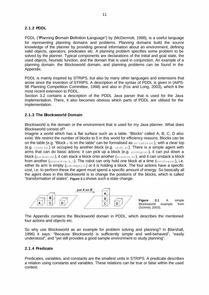
2.1.3 The Blocksworld Domain Blocksworld is the domain or the environment that is used for my Java planner. What does Blocksworld consist of? Imagine a world which has a flat surface such as a table. “Blocks” called A, B, C, D also exist. We restrict the number of blocks to 5 in this world for efficiency reasons. Blocks can be on the table (e.g. “Block a is on the table” can be formalised as on-table(a)), with a clear top (e.g. clear(a)) or occupied by another block (e.g. on(b,a)). There is a simple agent with arms that can do basic actions: it can pick up a block (e.g. pickup(a)), it can put down a block (putdown(a)), it can stack a block onto another (stack(a,b)), and it can unstack a block from another (unstack(a,b,)). The robot can only hold one block at a time (holding(a)), i.e. either its arm is empty (arm-empty()) or it is holding a block. The four actions have a specific cost, i.e. to perform these the agent must spend a specific amount of energy. So basically all the agent does in this Blocksworld is to change the positions of the blocks, which is called “transformation of states”. Figure 2.1 shows such a state change.

Figure 2.1 A simple Blocksworld example from (Schmid, 2003).

The Appendix contains the Blocksworld domain in PDDL, which describes the mentioned four actions and objects etc. So why use Blocksworld as an example for problem solving and planning? In (Marshall, 1996) it says: “Because Blocksworld is sufficiently simple and well-behaved”, “easily understood”, and “yet still provides a good sample environment to study planning”.

2.1.4 Predicate Predicates, variables, and constants are the smallest units in STRIPS. A predicate describes a relation using constants and variables. These relations can be true or false within the used context.

12

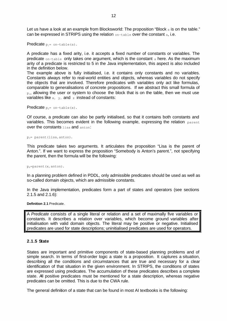
Let us have a look at an example from Blocksworld: The proposition “Block a is on the table.” can be expressed in STRIPS using the relation on-table over the constant a, i.e. Predicate p1= on-table(a). A predicate has a fixed arity, i.e. it accepts a fixed number of constants or variables. The predicate on-table only takes one argument, which is the constant a here. As the maximum arity of a predicate is restricted to 5 in the Java implementation, this aspect is also included in the definition below. The example above is fully initialised, i.e. it contains only constants and no variables. Constants always refer to real-world entities and objects, whereas variables do not specify the objects that are involved. Therefore predicates with variables only act like formulas, comparable to generalisations of concrete propositions. If we abstract this small formula of p1, allowing the user or system to choose the block that is on the table, then we must use variables like x, y, and z instead of constants: Predicate p2= on-table(x). Of course, a predicate can also be partly initialised, so that it contains both constants and variables. This becomes evident in the following example, expressing the relation parent over the constants lisa and anton: p3= parent(lisa,anton). This predicate takes two arguments. It articulates the proposition “Lisa is the parent of Anton.”. If we want to express the proposition “Somebody is Anton’s parent.”, not specifying the parent, then the formula will be the following: p4=parent(x,anton). In a planning problem defined in PDDL, only admissible predicates should be used as well as so-called domain objects, which are admissible constants. In the Java implementation, predicates form a part of states and operators (see sections 2.1.5 and 2.1.6): Definition 2.1 Predicate.

A Predicate consists of a single literal or relation and a set of maximally five variables or constants. It describes a relation over variables, which become ground variables after initialisation with valid domain objects. The literal may be positive or negative. Initialised predicates are used for state descriptions; uninitialised predicates are used for operators.

2.1.5 State States are important and primitive components of state-based planning problems and of simple search. In terms of first-order logic a state is a proposition. It captures a situation, describing all the conditions and circumstances that are true and necessary for a clear identification of that situation in the given environment. In STRIPS, the conditions of states are expressed using predicates. The accumulation of these predicates describes a complete state. All positive predicates must be mentioned for a state description, whereas negative predicates can be omitted. This is due to the CWA rule. The general definition of a state that can be found in most AI textbooks is the following:

13

Definition 2.2 State.

A State is a description of a situation, i.e. a conjunction of necessary positive Predicates. The Closed World Assumption (CWA) holds, i.e. unmentioned relations are false. Therefore all relevant predicates must be included in a state description. Let us have a look at a Blocksworld example in STRIPS: State s0= {on-table(x), clear(x), arm-empty()}. This is a state with three predicates. All predicates are uninitialised, so the state is uninstantiated. If we picturise this state, it will look like the following:

Figure 2.2 State s0.

Block x is on the table; it does not have any other blocks on top of it (it is “clear”), and no blocks are being held by the agent or robot (the arm is empty). Notice that block x can be any block since it does not denote a specific block yet (x is a variable, not a constant). So if a is a valid object or constant, s1={on-table(a), clear(a), arm-empty()} is a valid, instantiated state. Now, in Figure 2.3 block a exists in the defined environment.

Figure 2.3 State s1. Referring to the Java implementation, a state also possesses the following feature: Definition 2.3 Parent state of a state.

A state sn has exactly one link to its parent state or predecessor sn-1. A parent state is transformed to a successor state or a child after applying an operator o to it, so that on(sn-1)=sn. A state can have an infinite number of successor states. The parent state plays a crucial role in the generation of successor states (see 2.3.3) because predecessor states and their successors are connected via the parent link. Another issue is the generation of the solution path, which is done by chaining back from the goal state to the initial one by following the parent link of each state (see also next section for the operators). This way, the whole path can be generated. Figure 2.4 shows such an example.

Figure 2.4 Successor and predecessor states S with their parent links P.

2.1.6 Operator/Action Operators transform states to successor states, so that search can be performed and a search tree can be generated. Operators use so-called preconditions and effects. Preconditions describe the conditions that a state must contain or fulfil in order for the operator to be applicable. They are abbreviated as PRE. Effects (EFF) describe the changes that are applied to the current state to form the resulting new state. They are divided into an ADD-list and a DEL-list part. The ADD-list contains a set of positive predicates, whereas

14

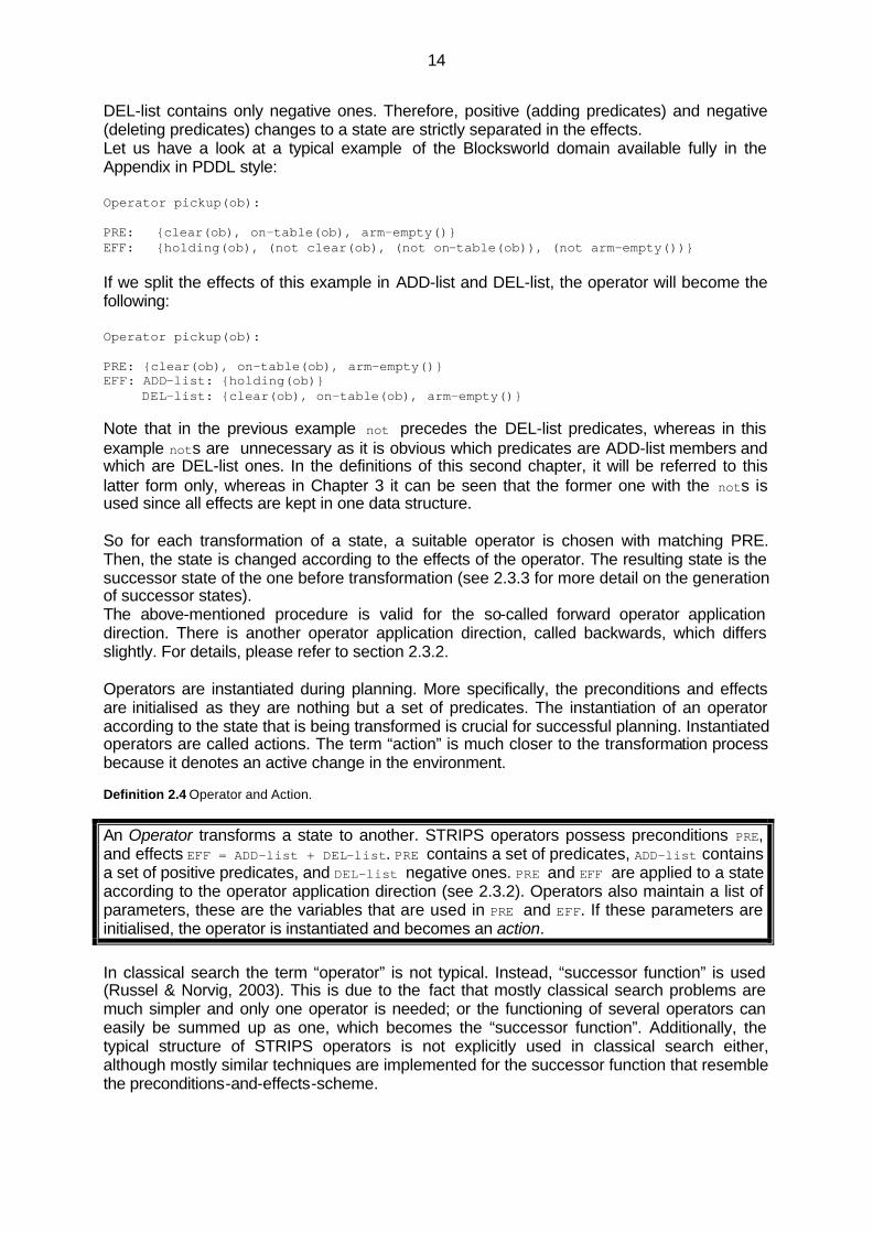
DEL-list contains only negative ones. Therefore, positive (adding predicates) and negative (deleting predicates) changes to a state are strictly separated in the effects. Let us have a look at a typical example of the Blocksworld domain available fully in the Appendix in PDDL style: Operator pickup(ob): PRE: {clear(ob), on-table(ob), arm-empty()} EFF: {holding(ob), (not clear(ob), (not on-table(ob)), (not arm-empty())} If we split the effects of this example in ADD-list and DEL-list, the operator will become the following: Operator pickup(ob): PRE: {clear(ob), on-table(ob), arm-empty()} EFF: ADD-list: {holding(ob)} DEL-list: {clear(ob), on-table(ob), arm-empty()} Note that in the previous example not precedes the DEL-list predicates, whereas in this example nots are unnecessary as it is obvious which predicates are ADD-list members and which are DEL-list ones. In the definitions of this second chapter, it will be referred to this latter form only, whereas in Chapter 3 it can be seen that the former one with the nots is used since all effects are kept in one data structure. So for each transformation of a state, a suitable operator is chosen with matching PRE. Then, the state is changed according to the effects of the operator. The resulting state is the successor state of the one before transformation (see 2.3.3 for more detail on the generation of successor states). The above-mentioned procedure is valid for the so-called forward operator application direction. There is another operator application direction, called backwards, which differs slightly. For details, please refer to section 2.3.2. Operators are instantiated during planning. More specifically, the preconditions and effects are initialised as they are nothing but a set of predicates. The instantiation of an operator according to the state that is being transformed is crucial for successful planning. Instantiated operators are called actions. The term “action” is much closer to the transformation process because it denotes an active change in the environment. Definition 2.4 Operator and Action.

An Operator transforms a state to another. STRIPS operators possess preconditions PRE, and effects EFF = ADD-list + DEL-list. PRE contains a set of predicates, ADD-list contains a set of positive predicates, and DEL-list negative ones. PRE and EFF are applied to a state according to the operator application direction (see 2.3.2). Operators also maintain a list of parameters, these are the variables that are used in PRE and EFF. If these parameters are initialised, the operator is instantiated and becomes an action. In classical search the term “operator” is not typical. Instead, “successor function” is used (Russel & Norvig, 2003). This is due to the fact that mostly classical search problems are much simpler and only one operator is needed; or the functioning of several operators can easily be summed up as one, which becomes the “successor function”. Additionally, the typical structure of STRIPS operators is not explicitly used in classical search either, although mostly similar techniques are implemented for the successor function that resemble the preconditions-and-effects-scheme.

15

2.1.7 Operator-State Pair As discussed in the last part, actions or instantiated operators transform a state to a successor state. Therefore it is useful to associate the resulting state and the operator with its initialised parameter(s). This is called operator-state pair. By doing this, it is possible to trace back the states and operators that have been generated during search, since predecessor and successor states are linked to each other via the parent link (see Definition 2.3). This is indispensable for the search tree and maintenance of the history of a search problem (see next part) and also for the search algorithms themselves (see 2.2). Definition 2.5 Operator-State Pair.

An Operator-State Pair is referred to as a Pair p=(o,s), and contains one instance of an operator o and a state s. O is the action that has been applied to s’ parent state to acquire s: on(sn-1)=sn.

Typical examples of operator-state pairs can be seen in Figures 3.7 and 3.8 in the next chapter.

2.1.8 Search Tree The search tree is an important data structure in problem solving, for it is used to record the whole search process accurately. Traditionally, the search tree is used to retain unexplored states only (Russel & Norvig, 1995), and some other data structure or list is reserved to maintain the set of explored states. These are called OPEN list and CLOSED list often in conjunction with best-first search strategies (see section 2.2.2). But on implementation grounds when it comes to programming, it is of advantage to maintain both in one data structure. This is why this type of search tree is preferred here (Definition 2.7). Before defining a search tree, one should first know about the state space. We are already familiar with predicates, states, and operators. The latter ones transform states to successors. Successors and the transforming actions are stored together as operator-state pairs. If we imagine the states of these operator-state pairs now as nodes of a tree, or as locations (dots) on a map, and the connections or operators between predecessor and successor states as lines or edges, then we can draw a complete tree or a map consisting of nodes and edges, or of dots and lines respectively. This is exactly what a state space is; it defines the set of all possible states and operators within a search or planning problem. That is, all possible state generations with the applied operators are gathered in a huge map. Starting from the initial state s0, which is kept in the operator-state pair p0=(null,s0) (there is no operator for the initial state for it does not have a predecessor state), one can follow any sequence of actions from one pair to another. Definition 2.6 State space.

The State space of a search or planning problem (see 2.3.1) contains the set of all existing states and operators that are valid within this problem. It consists of nodes (=states), which are linked by edges (=operators). A state and its immediately preceding operator are stored as an operator-state pair p=(o,s) in the state space. A search tree typically contains the operator-state pairs that are expanded from the state space during the search or planning process in a queue. These are called “explored states” in classical search. The search tree of Definition 2.9 always marks the current pair that is being explored, which starts with the initial pair p0. It proceeds from left to right, going from pair to pair as the search continues. New successor pairs are added to the right of the current pair always in correct order according to the search strategy. This way, the “history” of the search

16

process is stored left to the current pair, whereas unexplored pairs are added to its right. This data structure is applicable for all search strategies if one orders the successor pairs properly and adds them to the correct position in the tree (for more details see section 2.2). Definition 2.7 Search Tree and History.

A Search Tree ST represents the part of the state space that has been explored with a specific search strategy for a search problem. An index pos marks the current pair c that is being explored, which is initially set to pos=0. All the pairs p for which holds p(pos)<c(pos) define the history, i.e. the explored pairs, and all the pairs p for which holds p(pos)>c(pos) define the set of unexplored states. So formally, a search tree is a flattened list of pairs ST=(p0,…,pn), where p0=(null,s0) is the initial pair.

2.2 Classical Search In classical search problems the task is to find a solution path, i.e. a sequence of states that lead from the initial given state to the desired goal state. This is achieved by systematic search. Basic information about the problem is given as input: the so-called successor function (which acts as an operator), initial state, and goal state. The output is the solution path. The search technique relies on the chosen search strategy, of which there are two different kinds in problem solving: Uninformed and informed search. The former one searches the state space according to a fixed systematic order – it does not use further information about the problem for favouring nodes. Therefore uninformed search is also called blind search. Informed search is different: It includes special information about the problem, called heuristics, which increases the efficiency of the search process. Good nodes or paths are clearly favoured, bad ones are omitted and not elaborated on. The better the heuristics are, the better and faster the search will be performed. The current best informed search algorithm is A*. More on that will follow in this chapter.

2.2.1 Uninformed Search Algorithms As already mentioned, uninformed search algorithms search the state space according to a predetermined systematic order. There are many different algorithms, but all of them are mainly based on Breadth-First Search and Depth-First Search. These two strategies are explained in detail below because they are also relevant for my Java Blocksworld implementation. Other strategies that are extensions or combinations of the above-mentioned ones are the following (Russel & Norvig, 1995):

- Uniform cost search (combination of Breadth-First and Depth-First), - Depth-Limited (Depth-First Search with fixed maximal depth limit), - Iterative Deepening Search (Depth-Limited Search with increasing depth limit), - Bidirectional Search (searching forwards from the initial state and backwards from the

goal state) The definitions of the algorithms below only portray the core function addToTree. This function is sufficient for expressing a search strategy, since all it does is ordering the set of successor states in a specific way. Of course, a search strategy is only completely specified within the context of a proper main search algorithm. So please refer to section 2.3.4 for the main planning algorithm, where addToTree is included.

17

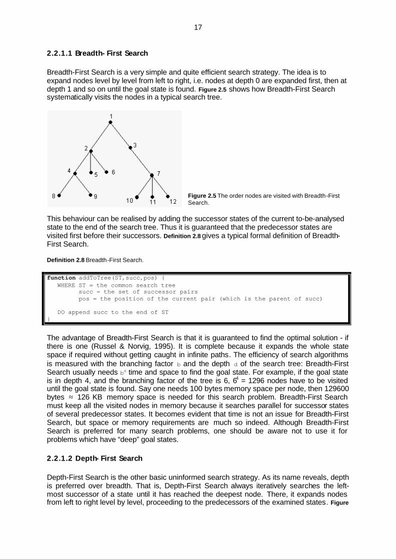
2.2.1.1 Breadth-First Search Breadth-First Search is a very simple and quite efficient search strategy. The idea is to expand nodes level by level from left to right, i.e. nodes at depth 0 are expanded first, then at depth 1 and so on until the goal state is found. Figure 2.5 shows how Breadth-First Search systematically visits the nodes in a typical search tree.

Figure 2.5 The order nodes are visited with Breadth-First Search.

This behaviour can be realised by adding the successor states of the current to-be-analysed state to the end of the search tree. Thus it is guaranteed that the predecessor states are visited first before their successors. Definition 2.8 gives a typical formal definition of Breadth-First Search. Definition 2.8 Breadth-First Search. function addToTree(ST,succ,pos) { WHERE ST = the common search tree succ = the set of successor pairs pos = the position of the current pair (which is the parent of succ) DO append succ to the end of ST }

The advantage of Breadth-First Search is that it is guaranteed to find the optimal solution - if there is one (Russel & Norvig, 1995). It is complete because it expands the whole state space if required without getting caught in infinite paths. The efficiency of search algorithms is measured with the branching factor b and the depth d of the search tree: Breadth-First Search usually needs bd time and space to find the goal state. For example, if the goal state is in depth 4, and the branching factor of the tree is 6, 64 = 1296 nodes have to be visited until the goal state is found. Say one needs 100 bytes memory space per node, then 129600 bytes ≈ 126 KB memory space is needed for this search problem. Breadth-First Search must keep all the visited nodes in memory because it searches parallel for successor states of several predecessor states. It becomes evident that time is not an issue for Breadth-First Search, but space or memory requirements are much so indeed. Although Breadth-First Search is preferred for many search problems, one should be aware not to use it for problems which have “deep” goal states.

2.2.1.2 Depth-First Search Depth-First Search is the other basic uninformed search strategy. As its name reveals, depth is preferred over breadth. That is, Depth-First Search always iteratively searches the left-most successor of a state until it has reached the deepest node. There, it expands nodes from left to right level by level, proceeding to the predecessors of the examined states. Figure

18

2.6 demonstrates how Depth-First Search systematically visits the nodes in a typical search tree.

Figure 2.6 The order nodes are visited with Depth-First Search.

Depth-First Search is typically implemented by adding the successor states of a state to the front of the search tree. This way it is assured that the newest successor states are expanded before their predecessors. Definition 2.9 seems to be different from this traditional approach – but actually it is not: Remember that our search tree (Definition 2.7) maintains both the history and the set of unexplored states. It also has a marker for the current state that is being explored (setting the border between the history and unexplored states), which is shifted to the right after every expansion. So according to this procedure one has to add the new successor states immediately after the current state – and not to the front of the search tree! Definition 2.9 Depth-First Search. function addToTree(ST,succ,pos) { WHERE ST = the common search tree succ = the set of successor pairs pos = the position of the current pair (which is the parent of succ) DO append succ at pos+1, shifting any successive pairs to the right }

Depth-First Search does not have the memory requirements of bd like Breadth-First Search. It usually only stores b*d nodes, which would be just 6*4 = 24 nodes in the above-mentioned example. Time requirements are the same as Breadth-First Search. But this is the only advantage: Depth-First Search is neither complete nor optimal, since it can get stuck in infinite loops! Imagine there was no goal state in the search tree of Figure 2.6, and node 4 had an infinite number of successor states. Then Depth-First Search would never finish as it would get stuck searching in the depth of the tree. Due to this reason Depth-First Search should not be chosen for problems which are known to have such infinite depths (Russel & Norvig, 1995).

2.2.2 Informed Search Algorithms Informed Search Algorithms use additional information about the search problem, a heuristic evaluation function. This function evaluates successor states by yielding a cost for them and thus helps in deciding which one to choose next. This cost stands for the remaining path costs that must be spent from the state to the goal state. Consequently, informed search algorithms differ from blind ones in that they do not use a fixed-order strategy, but some kind of “intelligent” information or knowledge for estimating successor states . The states or nodes are ordered such that the best ones (according to the evaluation function) are expanded first. (Russel & Norvig, 1995). Thus informed search algorithms are also called best-first search algorithms.

19

The performance of the best-first algorithm clearly depends on the heuristic function. Because of the heuristics, fewer states are expanded with a best-first algorithm than with a blind one, since the best-first algorithm does not require to “search” blindly. Time is not wasted by choosing redundant or irrelevant paths. The fewer steps are needed to obtain the solution path – i.e. the fewer states are expanded – the better the solution path will be. The aim of problem solving has always been to minimise the cost of search. So how to choose a good heuristic function? This depends on the problem on the one hand, but on the other hand there are some clear universal criteria that should be fulfilled:

1. A heuristic function should never overestimate the actual path costs. (Russel & Norvig, 1995).

2. The heuristic function should yield values for the remaining path cost that are as

close as possible to the actual ones. From this we can follow, that the heuristic function should yield as high values as possible, but it should not overestimate the actual ones. Such heuristics (especially fulfilling criterion 1 above) are called admissible (Russel & Norvig, 1995). The idea behind this underestimating heuristic function is that it will keep the search on the right track and ensure that the goal is reached. Section 2.3.6 covers heuristics functions for Blocksworld problems as an example. In order to perform informed search, states and operators must have additional information about costs. An operator has a fixed cost, which is the actual cost that is required to move from state A to state B. This is named g-cost. A state is assigned two different kinds of costs: The total amount of g-costs that has been spent to reach this state (g-cost), and the estimation of the heuristic function for the remaining path cost from this state to the goal state (h-cost). Definition 2.10 Cost information of a state.

A State s holds information about the actual cost that has been spent from the initial state s0 until s (g-cost), and the slightly underestimated cost that will be spent for the remaining path from s to the goal state sg (h-cost). Definition 2.11 Cost of an Operator.

An Operator o possesses a g-cost, which indicates the cost of moving from state s to successor state s’ with o. There are several types of best-first algorithms which differ in the usage of this heuristic function. Greedy Search and A* Search are described below.

2.2.2.1 Greedy Search Greedy Search is a very simple best-first algorithm. It aims at minimising the estimated path cost without taking into account the totally spent path cost (Russel & Norvig, 1995). In other words, this algorithm only utilises the h-cost but not the g-cost that is yielded by the operators. This is why it is said to be greedy; it chooses the seemingly best states without considering the whole result. Greedy Search can easily be implemented by ordering the successor states and the set of all unexplored states according to their h-cost so that the best successor states are guaranteed to be expanded first.

20

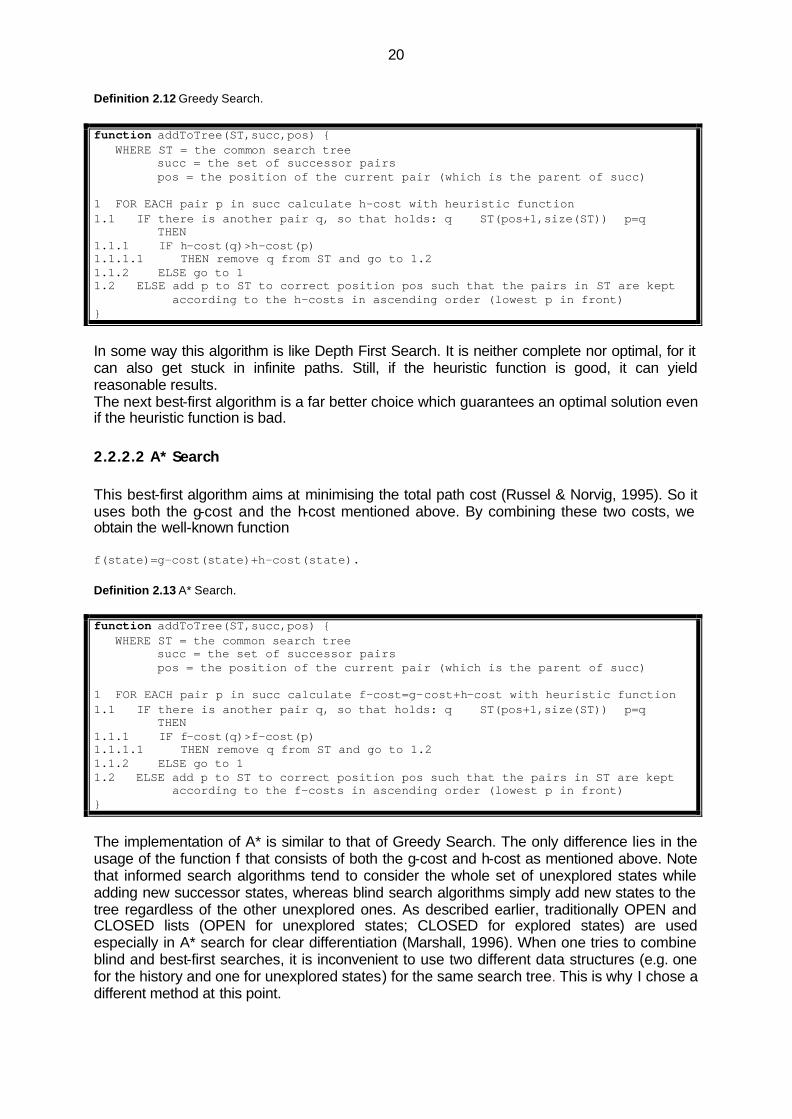
Definition 2.12 Greedy Search. function addToTree(ST,succ,pos) { WHERE ST = the common search tree succ = the set of successor pairs pos = the position of the current pair (which is the parent of succ) 1 FOR EACH pair p in succ calculate h-cost with heuristic function 1.1 IF there is another pair q, so that holds: q ∈ ST(pos+1,size(ST)) ∧ p=q THEN 1.1.1 IF h-cost(q)>h-cost(p) 1.1.1.1 THEN remove q from ST and go to 1.2 1.1.2 ELSE go to 1 1.2 ELSE add p to ST to correct position pos such that the pairs in ST are kept according to the h-costs in ascending order (lowest p in front) }

In some way this algorithm is like Depth First Search. It is neither complete nor optimal, for it can also get stuck in infinite paths. Still, if the heuristic function is good, it can yield reasonable results. The next best-first algorithm is a far better choice which guarantees an optimal solution even if the heuristic function is bad.

2.2.2.2 A* Search This best-first algorithm aims at minimising the total path cost (Russel & Norvig, 1995). So it uses both the g-cost and the h-cost mentioned above. By combining these two costs, we obtain the well-known function f(state)=g-cost(state)+h-cost(state). Definition 2.13 A* Search. function addToTree(ST,succ,pos) { WHERE ST = the common search tree succ = the set of successor pairs pos = the position of the current pair (which is the parent of succ) 1 FOR EACH pair p in succ calculate f-cost=g-cost+h-cost with heuristic function 1.1 IF there is another pair q, so that holds: q ∈ ST(pos+1,size(ST)) ∧ p=q THEN 1.1.1 IF f-cost(q)>f-cost(p) 1.1.1.1 THEN remove q from ST and go to 1.2 1.1.2 ELSE go to 1 1.2 ELSE add p to ST to correct position pos such that the pairs in ST are kept according to the f-costs in ascending order (lowest p in front) }

The implementation of A* is similar to that of Greedy Search. The only difference lies in the usage of the function f that consists of both the g-cost and h-cost as mentioned above. Note that informed search algorithms tend to consider the whole set of unexplored states while adding new successor states, whereas blind search algorithms simply add new states to the tree regardless of the other unexplored ones. As described earlier, traditionally OPEN and CLOSED lists (OPEN for unexplored states; CLOSED for explored states) are used especially in A* search for clear differentiation (Marshall, 1996). When one tries to combine blind and best-first searches, it is inconvenient to use two different data structures (e.g. one for the history and one for unexplored states) for the same search tree. This is why I chose a different method at this point.

21

A* is optimal and complete because it always finds the cheapest solution. This is because it basically both looks back an forth, and does not make its decisions blindly. A* combines the features of uniform cost search and the heuristic function.

2.3 State-Based Planning State-based planning uses problem-solving basics for a broader type of searching: Planning. Planning allows different operator application directions, diverse search strategies, and most important – a planner can easily be combined with numerous domain and problem files. We defined the output of a search problem as the “solution path”, i.e. a sequence of actions starting from the initial state and leading to the goal state. Now in planning, we call the output a plan. The emphasis here does not reside in the goal state that we obtain, or just the solution path. The solution represents the whole strategy or approach that has been undertaken to solve the given problem. As a result, plans can be complete or incomplete (partial plans) for one can record the planning process and store it easily. This is useful if one has to change the strategy because the applied one is not optimal. Planning problems tend to be more complex than search problems, so being able to decompose the problem is crucial in planning (Rich & Knight, 1991). However, search problems have to be finished and cannot be altered once the search has been executed. One cannot recover a search process effortlessly and continue searching from any arbitrary position. In this last part of the chapter, the components of sections 2.1 and 2.2 are integrated into the main planning concept and become a complete system which can be used for solving problems eventually. Special topics are elaborated that are required for the main planning algorithm. At last, it is dealt with Blocksworld specific issues.

2.3.1 Planning Problem The term “planning problem” corresponds to the contents of problem and domain files in PDDL. There, all the information that is problem specific is included in the problem file, whereas domain specific knowledge is available in the domain file. Here, we deal with both information in a PDDL-independent format. The input to a planner is a “planning problem” as defined in Definition 2.14. As mentioned before, there are different kinds of planners. A partial order planner does not require a fixed ordering for all actions and partly instantiated plans are allowed, whereas a total order planner accepts only a strict ordering of applied actions. That is, a finished plan must be fully instantiated so that no alteration is possible (Russel & Norvig, 1995). Note that actually total order planners accept a set of initial states I and goal states G, but my Java implementation restricts this to one each (as in Definition 2.14).

22

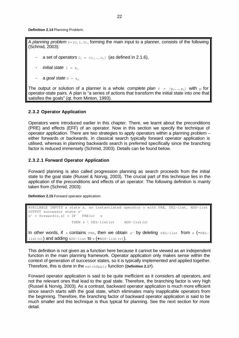
Definition 2.14 Planning Problem.

A planning problem P=(O,I,G), forming the main input to a planner, consists of the following (Schmid, 2003):

- a set of operators Oi = {o1,…,on} (as defined in 2.1.6), - initial state I = so, - a goal state G = sg.

The output or solution of a planner is a whole complete plan P = {p0,…,pg} with p for operator-state pairs. A plan is “a series of actions that transform the initial state into one that satisfies the goals” (qt. from Minton, 1993).

2.3.2 Operator Application Operators were introduced earlier in this chapter. There, we learnt about the preconditions (PRE) and effects (EFF) of an operator. Now in this section we specify the technique of operator application. There are two strategies to apply operators within a planning problem – either forwards or backwards. In classical search typically forward operator application is utilised, whereas in planning backwards search is preferred specifically since the branching factor is reduced immensely (Schmid, 2003). Details can be found below.

2.3.2.1 Forward Operator Application Forward planning is also called progression planning as search proceeds from the initial state to the goal state (Russel & Norvig, 2003). The crucial part of this technique lies in the application of the preconditions and effects of an operator. The following definition is mainly taken from (Schmid, 2003): Definition 2.15 Forward operator application. AVAILABLE INPUTS a state s, an instantiated operator o with PRE, DEL-list, ADD-list OUTPUT successor state s’ s’ = forward(o,s) = IF PRE(o) ⊆ s

THEN s \ DEL-list(o) ∪ ADD-list(o) In other words, if s contains PRE, then we obtain s’ by deleting DEL-list from s (-DEL-list(o)) and adding ADD-list to s (+ADD-list(o)).

This definition is not given as a function here because it cannot be viewed as an independent function in the main planning framework. Operator application only makes sense within the context of generation of successor states, so it is typically implemented and applied together. Therefore, this is done in the matchApply function (Definition 2.17). Forward operator application is said to be quite inefficient as it considers all operators, and not the relevant ones that lead to the goal state. Therefore, the branching factor is very high (Russel & Norvig, 2003). As a contrast, backward operator application is much more efficient since search starts with the goal state, which eliminates many inapplicable operators from the beginning. Therefore, the branching factor of backward operator application is said to be much smaller and this technique is thus typical for planning. See the next section for more detail.

23

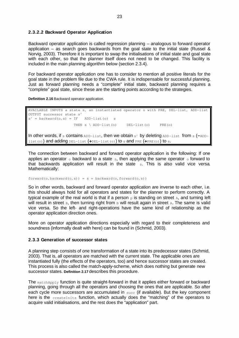
2.3.2.2 Backward Operator Application Backward operator application is called regression planning – analogous to forward operator application – as search goes backwards from the goal state to the initial state (Russel & Norvig, 2003). Therefore it is important to swap the initialisations of initial state and goal state with each other, so that the planner itself does not need to be changed. This facility is included in the main planning algorithm below (section 2.3.4). For backward operator application one has to consider to mention all positive literals for the goal state in the problem file due to the CWA rule. It is indispensable for successful planning. Just as forward planning needs a “complete” initial state, backward planning requires a “complete” goal state, since these are the starting points according to the strategies. Definition 2.16 Backward operator application. AVAILABLE INPUTS a state s, an instantiated operator o with PRE, DEL-list, ADD-list OUTPUT successor state s’ s’ = backward(o,s) = IF ADD-list(o)⊆ s

THEN s \ ADD-list(o) ∪ DEL-list(o) ∪ PRE(o) In other words, if s contains ADD-list, then we obtain s’ by deleting ADD-list from s (-ADD-list(o)) and adding DEL-list (+DEL-list(o)) to s and PRE (+PRE(o)) to s.

The connection between backward and forward operator application is the following: If one applies an operator o backward to a state s, then applying the same operator o forward to that backwards application will result in the state s. This is also valid vice versa. Mathematically: forward(o,backward(o,s)) = s = backward(o,forward(o,s)) So in other words, backward and forward operator application are inverse to each other, i.e. this should always hold for all operators and states for the planner to perform correctly. A typical example of the real world is that if a person p is standing on street A, and turning left will result in street B, then turning right from B will result again in street A. The same is valid vice versa. So the left- and right-operations have the same kind of relationship as the operator application direction ones. More on operator application directions especially with regard to their completeness and soundness (informally dealt with here) can be found in (Schmid, 2003).

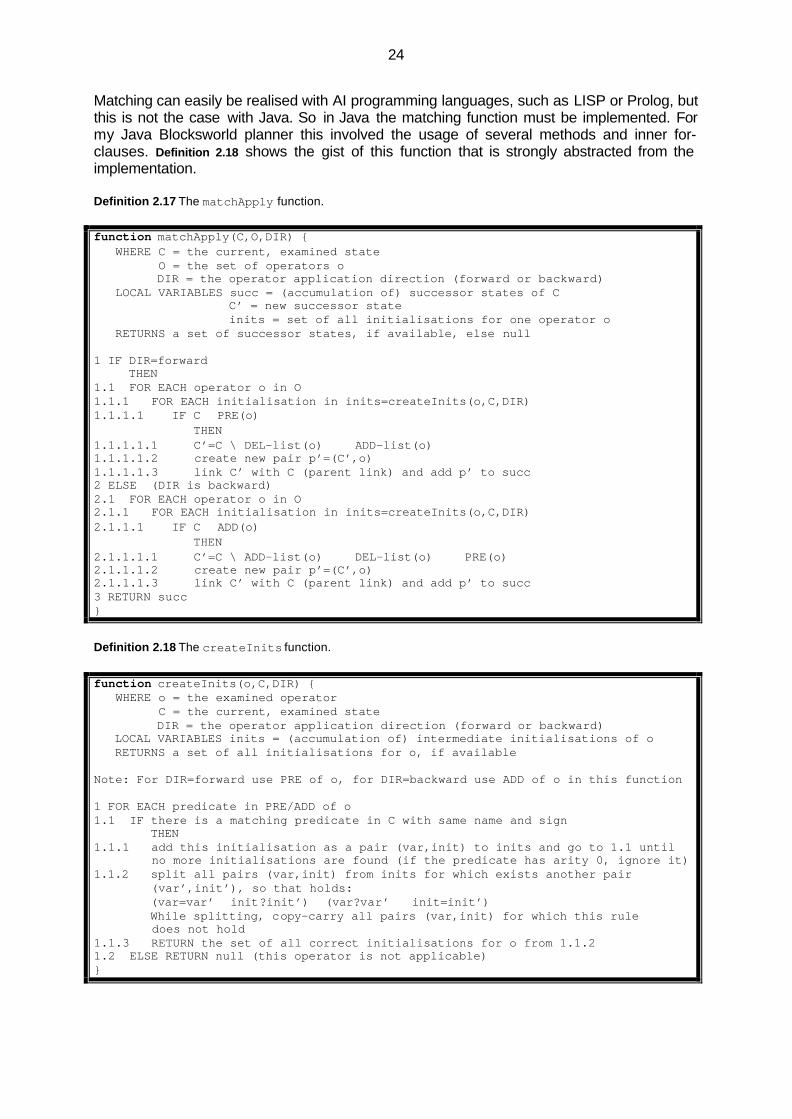
2.3.3 Generation of successor states A planning step consists of one transformation of a state into its predecessor states (Schmid, 2003). That is, all operators are matched with the current state. The applicable ones are instantiated fully (the effects of the operators, too) and hence successor states are created. This process is also called the match-apply-scheme, which does nothing but generate new successor states. Definition 2.17 describes this procedure. The matchApply function is quite straight-forward in that it applies either forward or backward planning, going through all the operators and choosing the ones that are applicable. So after each cycle more successors are accumulated in succ (if available). But the key component here is the createInits function, which actually does the “matching” of the operators to acquire valid initialisations, and the rest does the “application” part.

24

Matching can easily be realised with AI programming languages, such as LISP or Prolog, but this is not the case with Java. So in Java the matching function must be implemented. For my Java Blocksworld planner this involved the usage of several methods and inner for-clauses. Definition 2.18 shows the gist of this function that is strongly abstracted from the implementation. Definition 2.17 The matchApply function. function matchApply(C,O,DIR) { WHERE C = the current, examined state O = the set of operators o DIR = the operator application direction (forward or backward) LOCAL VARIABLES succ = (accumulation of) successor states of C C’ = new successor state inits = set of all initialisations for one operator o RETURNS a set of successor states, if available, else null 1 IF DIR=forward THEN 1.1 FOR EACH operator o in O 1.1.1 FOR EACH initialisation in inits=createInits(o,C,DIR) 1.1.1.1 IF C ⊆ PRE(o) THEN 1.1.1.1.1 C’=C \ DEL-list(o) ∪ ADD-list(o) 1.1.1.1.2 create new pair p’=(C’,o) 1.1.1.1.3 link C’ with C (parent link) and add p’ to succ 2 ELSE (DIR is backward) 2.1 FOR EACH operator o in O 2.1.1 FOR EACH initialisation in inits=createInits(o,C,DIR) 2.1.1.1 IF C ⊆ ADD(o) THEN 2.1.1.1.1 C’=C \ ADD-list(o) ∪ DEL-list(o) ∪ PRE(o) 2.1.1.1.2 create new pair p’=(C’,o) 2.1.1.1.3 link C’ with C (parent link) and add p’ to succ 3 RETURN succ } Definition 2.18 The createInits function. function createInits(o,C,DIR) { WHERE o = the examined operator C = the current, examined state DIR = the operator application direction (forward or backward) LOCAL VARIABLES inits = (accumulation of) intermediate initialisations of o RETURNS a set of all initialisations for o, if available Note: For DIR=forward use PRE of o, for DIR=backward use ADD of o in this function 1 FOR EACH predicate in PRE/ADD of o 1.1 IF there is a matching predicate in C with same name and sign THEN 1.1.1 add this initialisation as a pair (var,init) to inits and go to 1.1 until no more initialisations are found (if the predicate has arity 0, ignore it) 1.1.2 split all pairs (var,init) from inits for which exists another pair (var’,init’), so that holds: (var=var’ ∧ init?init’) ∨ (var?var’ ∧ init=init’) While splitting, copy-carry all pairs (var,init) for which this rule does not hold 1.1.3 RETURN the set of all correct initialisations for o from 1.1.2 1.2 ELSE RETURN null (this operator is not applicable) }

25

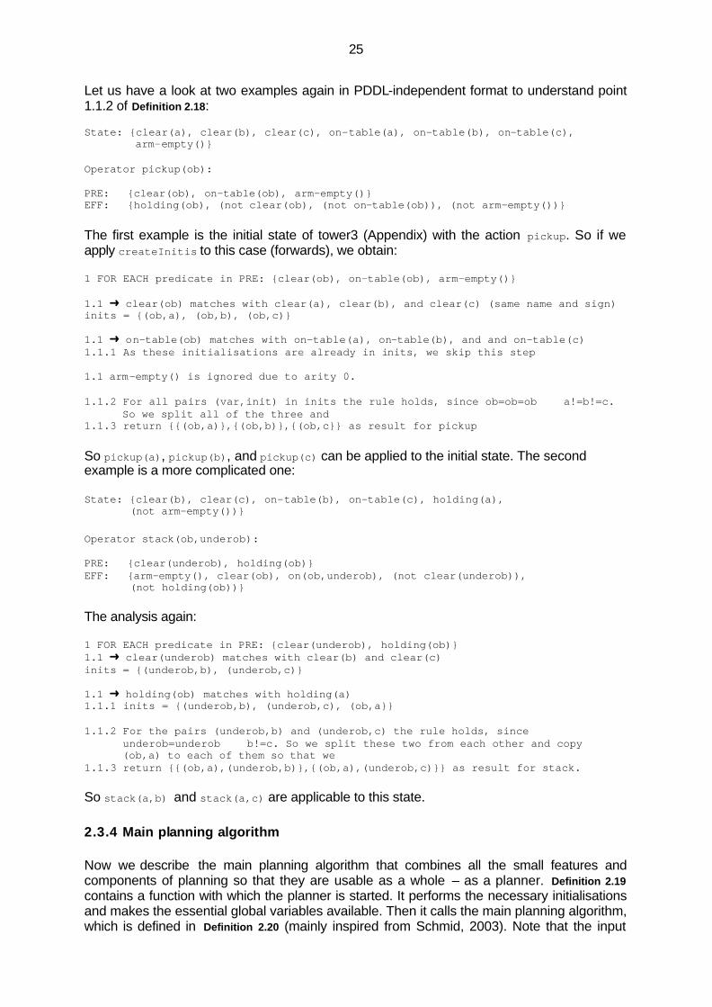
Let us have a look at two examples again in PDDL-independent format to understand point 1.1.2 of Definition 2.18: State: {clear(a), clear(b), clear(c), on-table(a), on-table(b), on-table(c), arm-empty()} Operator pickup(ob): PRE: {clear(ob), on-table(ob), arm-empty()} EFF: {holding(ob), (not clear(ob), (not on-table(ob)), (not arm-empty())} The first example is the initial state of tower3 (Appendix) with the action pickup. So if we apply createInitis to this case (forwards), we obtain: 1 FOR EACH predicate in PRE: {clear(ob), on-table(ob), arm-empty()} 1.1 Ü clear(ob) matches with clear(a), clear(b), and clear(c) (same name and sign) inits = {(ob,a), (ob,b), (ob,c)} 1.1 Ü on-table(ob) matches with on-table(a), on-table(b), and and on-table(c) 1.1.1 As these initialisations are already in inits, we skip this step 1.1 arm-empty() is ignored due to arity 0. 1.1.2 For all pairs (var,init) in inits the rule holds, since ob=ob=ob ∧ a!=b!=c. So we split all of the three and 1.1.3 return {{(ob,a)},{(ob,b)},{(ob,c}} as result for pickup So pickup(a), pickup(b), and pickup(c) can be applied to the initial state. The second example is a more complicated one: State: {clear(b), clear(c), on-table(b), on-table(c), holding(a), (not arm-empty())} Operator stack(ob,underob): PRE: {clear(underob), holding(ob)} EFF: {arm-empty(), clear(ob), on(ob,underob), (not clear(underob)), (not holding(ob))} The analysis again: 1 FOR EACH predicate in PRE: {clear(underob), holding(ob)} 1.1 Ü clear(underob) matches with clear(b) and clear(c) inits = {(underob,b), (underob,c)} 1.1 Ü holding(ob) matches with holding(a) 1.1.1 inits = {(underob,b), (underob,c), (ob,a}} 1.1.2 For the pairs (underob,b) and (underob,c) the rule holds, since underob=underob ∧ b!=c. So we split these two from each other and copy (ob,a) to each of them so that we 1.1.3 return {{(ob,a),(underob,b)},{(ob,a),(underob,c)}} as result for stack. So stack(a,b) and stack(a,c) are applicable to this state.

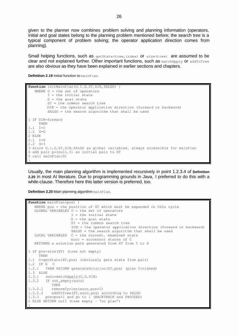
2.3.4 Main planning algorithm Now we describe the main planning algorithm that combines all the small features and components of planning so that they are usable as a whole – as a planner. Definition 2.19 contains a function with which the planner is started. It performs the necessary initialisations and makes the essential global variables available. Then it calls the main planning algorithm, which is defined in Definition 2.20 (mainly inspired from Schmid, 2003). Note that the input

26

given to the planner now combines problem solving and planning information (operators, initial and goal states belong to the planning problem mentioned before; the search tree is a typical component of problem solving; the operator application direction comes from planning). Small helping functions, such as getState(tree,index) or size(tree) are assumed to be clear and not explained further. Other important functions, such as matchApply or addToTree are also obvious as they have been explained in earlier sections and chapters. Definition 2.19 Initial function to mainPlan. function initMainPlan(O,I,G,ST,DIR,SALGO) { WHERE O = the set of operators I = the initial state G = the goal state ST = the common search tree DIR = the operator application direction (forward or backward) SALGO = the search algorithm that shall be used 1 IF DIR=forward THEN 1.1 I=I 1.2 G=G 2 ELSE 2.1 I=G 2.2 G=I 3 store O,I,G,ST,DIR,SALGO as global variables, always accessible for mainPlan 4 add pair p=(null,I) as initial pair to ST 5 call mainPlan(0) }

Usually, the main planning algorithm is implemented recursively in point 1.2.3.4 of Definition 2.20 in most AI literature. Due to programming grounds in Java, I preferred to do this with a while-clause. Therefore here this latter version is preferred, too. Definition 2.20 Main planning algorithm mainPlan. function mainPlan(pos) { WHERE pos = the position of ST which must be expanded in this cycle GLOBAL VARIABLES O = the set of operators I = the initial state G = the goal state ST = the common search tree DIR = the operator application direction (forward or backward) SALGO = the search algorithm that shall be used LOCAL VARIABLES C = the current, examined state succ = successor states of C RETURNS a solution path generated from ST from I to G 1 IF pos<size(ST) (tree not empty) THEN 1.1 C=getState(ST,pos) (obviously gets state from pair) 1.2 IF G ⊆ C 1.2.1 THEN RETURN generateSolution(ST,pos) (plan finished) 1.3 ELSE 1.3.1 succ=matchApply(C,O,DIR) 1.3.2 IF not_empty(succ) THEN 1.3.2.1 removeCycles(succ,pos+1) 1.3.2.2 addToTree(ST,succ,pos) according to SALGO 1.3.3 pos=pos+1 and go to 1 (BACKTRACK and PROCEED) 2 ELSE RETURN null (tree empty – “no plan”) }

27

A planner that is programmed according to this main planning algorithm will find a solution, if there is one, else it will quit without a solution. Backtracking to the last choice point and proceeding to the next state are possible without any efforts or fussy search. This is due to the structure of the search tree, which maintains both the history and explored states, but it is also due to the compatibility of the planning algorithm with several search strategies. Backtracking becomes necessary if a currently examined state does not possess any successors and if it does not contain the goal state. At this point, one must backtrack to the last choice point, to the set of unexplored “sister states” of the last predecessor that was examined. Proceeding to the next state simply means expanding the current successor state. The function removeCycles(succ, pos+1) removes all double pairs pi=(oi,si) from the set of successor states succ, which are also contained in the history (this holds for all search algorithms except for the informed search ones where the whole search tree, i.e. history plus unexplored states must be considered). Thus, it is guaranteed that there are no cycles in the search tree which would lead to a never terminating planner.

2.3.5 Some Blocksworld Problems In section 2.1.3 the Blocksworld domain was introduced, and throughout the chapter several examples were given. The Appendix contains several Blocksworld problem files in PDDL, like tower2, two tower3 problems, and tower4, which are picturised below.

Figure 2.7 tower2 (see Appendix). Figure 2.8 tower3 (see Appendix).

Figure 2.9 variant of tower3 (see Appendix). Figure 2.10 tower4 (see Appendix). The approach that is taken is always the same: We choose one problem file, formulate it in a language that our planner understands (e.g. PDDL), choose a search strategy, and an operator application direction. Then we let the planner perform the search and return the solution path that contains all the operator state pairs that were used to construct the plan. The next chapter contains screen shots of such example runs with the problems above (or one can also test it oneself by running the planner provided on the CD).

2.3.6 Blocksworld Heuristics for Informed Search Recall that in section 2.2.2 when describing informed search algorithms, we introduced heuristics. A good heuristic function determines the performance of the best-first algorithm. Turning now to our well-known domain, Blocksworld: How could a good heuristic function for the Blocksworld domain look like? How to create such a function? The basic approach to finding a good heuristic function is to “look at the effects of the actions and the goals that must be achieved and to guess how many actions are needed to achieve

28

all the goals” (qt. from Russel & Norvig, 2003). But this is not as straight-forward as it sounds. A heuristic function cannot be that precise to judge exactly how many steps still must be taken after a specific action. One thing is certain: Finding a good heuristic function for Blocksworld is difficult. One sub-aim is to choose an admissible heuristics, i.e. one that never overestimates the actual costs that are required. The easiest way to do this is to manually favour the best states. This has been done for the implementation of A* in the underlying planner. For A*, costs are distributed according to the total cost f. For each choice point, one has to assign the lowest cost to the state that shall be favoured. Thus, it is always guaranteed that the heuristics will be optimal. The examples are available in full length in the Appendix (under “Blocksworld problem files”), but let us have a look at the simple heuristics part of “tower2” to get an impression about how to distribute the costs: (:heuristics (on-table a) (on-table b) (clear a) (clear b) (arm-empty) 4 (on-table b) (clear b) (holding a) 2 (on-table a) (clear a) (holding b) 5 (arm-empty) (on a b) (on-table b) (clear a) 0 (arm-empty) (on b a) (on-table a) (clear b) 5 ) The heuristics resembles a table, where for each possible state in the state space a cost has to be given (h-cost). The costs are mentioned here after each state. Additionally, the actions must also have costs (g-cost). They are abbreviated here (also available in full length in the Appendix). (:action pickup (:action putdown (:action stack (:action unstack :cost (1) :cost (3) :cost (1) :cost (4) …) …) …) …) Figure 2.7 shows the search tree for tower 2 with costs at each edge.

Figure 2.7 The search tree of tower2 with costs.

Here, the first cost of the equations mentioned next to the arrows is the g-cost of the operator, the second one is the h-cost of the next state. It is evident that A* chooses the left path of this tree as pickup(A) is cheaper than pickup(B), and then after one more step it will have reached the goal state anyway. So in order to create a good heuristic function by hand, one must favour the best path. Still, for more complex problems than tower2, it is necessary to check whether the assigned costs are unequivocal and that no other path can be chosen than the intended one.

29

Note that tower4 available in the Appendix does not contain any heuristics as it already finds the optimal solution (it behaves like Breadth-First Search without heuristics). There are also some “real” approaches to Blocksworld heuristics with functions that do not work with a table but “judge” a state according to specific rules. In (Rieksts, 2002) it is proposed to count the blocks in a state that must be moved twice. So, the heuristic function would be h = N(1) + N(2) where N(1) is the number of blocks that must be moved, and N(2) is the number of blocks that must be moved twice. The question here is how to decide which blocks must be moved twice. One idea is to count the number of blocks which a block depends on, i.e. it cannot be moved before those blocks are moved. As one can see, the most accurate heuristics can be obtained by choosing a “hand-made” one. This method is also much more efficient as only the lookup time to the table is spent. The drawback is that one has to include all states of the state space in the table manually. As a contrast, such functions as shown above might be easy to program but they might take much calculation time to consider all the cases that influence the cost.

30

3 Implementation of the planner This chapter gives an insight into the programming code in Java provided on the CD that comes with this paper. The Java planner implements the concepts and definitions discussed in Chapter 2. Blocksworld examples introduced in section 2.3.5 are available for testing with forward and backward operator application directions – with breadth-first search, depth-first search, and A* search algorithms. The functioning of the planner is shown by screen shots from an example run with tower3, breadth-first search, and forward operator application. Additionally, this chapter is concerned with the non-problem solving and planning parts, such as parsing PDDL code to Java. User interaction with the interface (applet) is shown in the last part of this chapter.

3.1 Overview of Classes Figure 3.1 and Figure 3.2 give a general view of the classes that are involved, showing their structure and components.

Figure 3.1 An abridged UML diagram of PlannerApplet.java and its interactions. PlannerApplet.java contains the code of the applet, which provides an environment for the planner for obtaining user input and showing the output of the solution. The planning process is started by calling Planner.java with the relevant information that is required. Therefore Planner.java acts as the main method of the planning process. The package bscproj as shown in Figure 3.2 contains all the parsing and planning classes. Parsing classes are LexicalAnalyser.java and SyntaxAnalyser.java. They translate PDDL code to Java, which is dealt with in 3.2 in more detail. All the other classes belong to the planner. Details about the concepts and algorithms that were used are given in Chapter 2 formally, or in pseudo code respectively.

31

Figure 3.2 UML diagram of the package bscproj.

32

3.2 Parsing PDDL to Java PDDL is a typical language for describing planning problems as discussed in 2.2.3. The target language for the underlying Blocksworld planner is Java, so the PDDL input has to be translated into it. This is done by the parser classes in bscproj (see 3.1). The used parser is a simple top-down left-to-right one-token-lookahead parser. It analyses the input code and creates code in Java accordingly. Analysis is done in two steps, first on a lexical basis, i.e. tokens are recognised. Then the analysis is performed on a syntactical level. This is realised by lexical and syntax analysers, which are described in this chapter. Top-down predictive parsers have been proven to be very easy to implement for it is guaranteed that the correct code is chosen at all times (Watson, 2001). This is important for the parser’s efficiency because backtracking is very costly and complicates the code. This technique was utilised to implement the parser for the planner. Unfortunately – according to the PDDL grammars specified in Figure 3.4 and Figure 3.5 – sometimes it was necessary to look two tokens ahead. Still, the parser is deterministic and tackles these problems.

3.2.1 Lexical Analyser LexicalAnalyser.java represents this part. The main work this class does is recognising tokens that are used in PDDL input files, namely the following ones:

Additional information for tokens 20-23: A <Variable> is recognised with the starting symbol "?". Then its name is parsed and stored as a string (according to <Name>). A <Name> is an arbitrary string that starts with a letter and is not one of the reserved tokens 0-19. Additionally, it must not be longer than 20 characters. Its value is stored as a String. A <Number> is a number of maximally two digits. Its value is stored as an int. An <Error> represents an error message which can be produced by both the lexical analyser and syntax analyser after either reading an invalid token (including too long <Name>s and <Variable>s) or if a syntax error is encountered. Figure 3.3 Encoding of tokens: Symbol table.

Each token type is encoded with a special integer. This information is used by the syntax analyser for parsing a PDDL file (see next section). Tokens 1-19 are “reserved”, i.e. if they are intended to be used as variables or in any other context than the intended one, the lexical analyser will complain. Tokens 20-23 are special tokens, as they also have a so-called “token value”. This is used to store values that names,

token type Meaning “has value” 0 define No 1 domain No 2 not No 3 and No 4 problem No 5 :requirements No 6 :strips No 7 :predicates No 8 :action No 9 :parameters No 10 :precondition No 11 :effect No 12 :domain No 13 :objects No 14 :init No 15 :goal No 16 :cost No 17 :heuristics No 18 ( No 19 ) No 20 ?<Variable> Yes 21 <Name> Yes 22 <Number> Yes 23 <Error> Yes

33

variables, numbers, and error messages refer to. This information is processed by the syntax analyser. Spaces, tabs, new lines, and comments are recognised and ignored by the lexical analyser. Therefore they do not need to be encoded.

3.2.2 Syntax Analyser SyntaxAnalyser.java represents the syntax analyser. It requests tokens from the lexical analyser whenever it is needed, and parses those according to the EBNF grammar rules specified in Figure 3.4 and Figure 3.5. First, the domain file is parsed always, followed by the problem file. The Appendix contains descriptions of the syntactic notation that has been used for the EBNF grammars. Furthermore, the following conventions hold within the SyntaxAnalyser.java class: Comments begin with a semicolon ";" and end at the end of the line. They will be ignored

by the parser. File Only one PDDL domain or problem specification may occur in a single file. Requirements If the requirements field is missing, :strips is used. Variables Actions: Only variables that have been declared in the parameters section of

the action description may be used. Free variables are not allowed. At most 5 variables are allowed for one predicate.

Parameters The number of parameters is restricted to 5 in the implementation. Objects used in the :init and :goal fields must be declared in the :objects field (see

Figure 3.4). The grammars in Figures 3.4 and 3.5 define a subset of PDDL 1.2 as it is required for the planner. Only the most important features of PDDL v1.2 are utilised, such as basic STRIPS-style actions. Other requirements are not supported. Problem files also use some of the non-terminals specified in Figure 3.4. Domain = "(" "define" "(" "domain" Name ")" [Requirements] Predicates Actions

{Actions} ")". Requirements = "(" ":requirements" ":strips" ")". Predicates = "(" ":predicates" PredDef {PredDef} ")". PredDef = "(" Name {Variable} ")". Actions = "(" ":action" Name [":cost" "(" Number ")"] ":parameters" "(" {Variable} ")" [Precondition] [Effect] ")". Precondition = ":precondition" EffectGoalDef. Effect = ":effect" EffectGoalDef. EffectGoalDef = Literal | "(" "and" {EffectGoalDef} ")". Literal = "(" "not" PredDef ")" | PredDef. Name = Letter {Letter | Digit | Special}. Number = Digit [Digit]. Variable = "?" Name. Letter = "A" | "B" | "C" | "D" | "E" | "F" | "G" | "H" | "I" | "J" | "K" | "L" |

"M" | "N" | "O" | "P" | "Q" | "R" | "S" | "T" | "U" | "V" | "W" | "X" | "Y" | "Z" | "a" | "b" | "c" | "d" | "e" | "f" | "g" | "h" | "i" | "j" | "k" | "l" | "m" | "n" | "o" | "p" | "q" | "r" | "s" | "t" | "u" | "v" | "x" | "y" | "z".

Digit = "0" | "1" | "2" | "3" | "4" | "5" | "6" | "7" | "8" | "9". Special = "-" | "_". Figure 3.4 EBNF description for domain files. As mentioned in the beginning of this chapter, a one-token-lookahead parser is not sufficient at all times. Many rules start with an open bracket. If there are choice points where one has to decide which rule to choose of two – and both start with the same terminal symbol, then the above-mentioned parser cannot be deterministic anymore. In these two EBNF grammars here we encounter this problem since many rules start with an open bracket. The affected

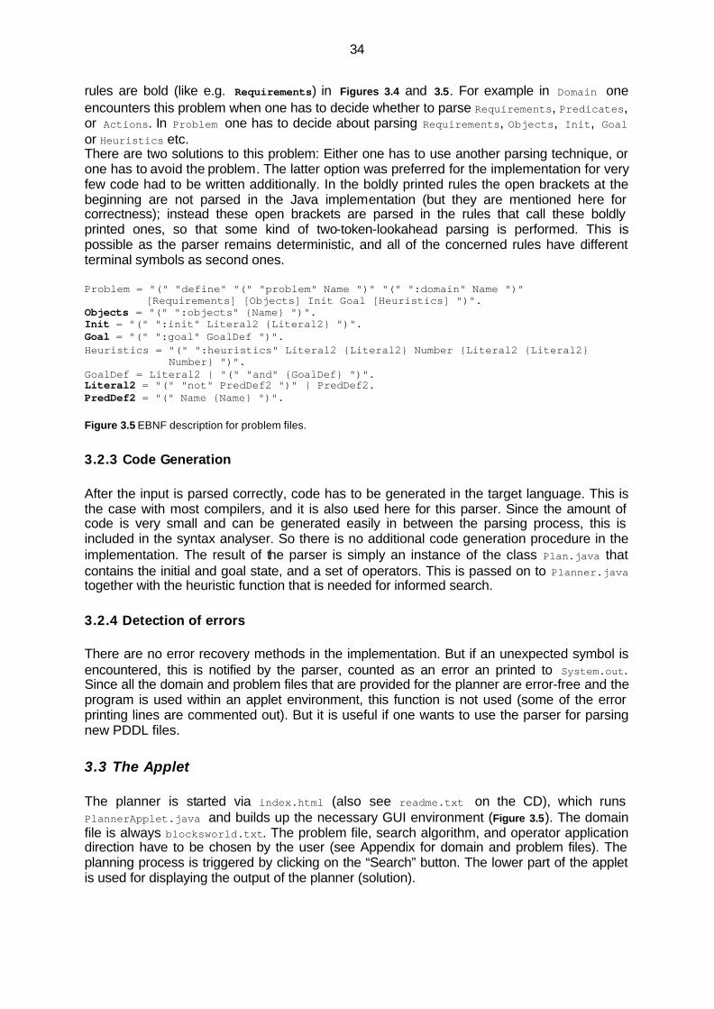
34

rules are bold (like e.g. Requirements) in Figures 3.4 and 3.5. For example in Domain one encounters this problem when one has to decide whether to parse Requirements, Predicates, or Actions. In Problem one has to decide about parsing Requirements, Objects, Init, Goal or Heuristics etc. There are two solutions to this problem: Either one has to use another parsing technique, or one has to avoid the problem. The latter option was preferred for the implementation for very few code had to be written additionally. In the boldly printed rules the open brackets at the beginning are not parsed in the Java implementation (but they are mentioned here for correctness); instead these open brackets are parsed in the rules that call these boldly printed ones, so that some kind of two-token-lookahead parsing is performed. This is possible as the parser remains deterministic, and all of the concerned rules have different terminal symbols as second ones. Problem = "(" "define" "(" "problem" Name ")" "(" ":domain" Name ")"

[Requirements] [Objects] Init Goal [Heuristics] ")". Objects = "(" ":objects" {Name} ")". Init = "(" ":init" Literal2 {Literal2} ")". Goal = "(" ":goal" GoalDef ")". Heuristics = "(" ":heuristics" Literal2 {Literal2} Number {Literal2 {Literal2} Number} ")". GoalDef = Literal2 | "(" "and" {GoalDef} ")". Literal2 = "(" "not" PredDef2 ")" | PredDef2. PredDef2 = "(" Name {Name} ")". Figure 3.5 EBNF description for problem files.

3.2.3 Code Generation After the input is parsed correctly, code has to be generated in the target language. This is the case with most compilers, and it is also used here for this parser. Since the amount of code is very small and can be generated easily in between the parsing process, this is included in the syntax analyser. So there is no additional code generation procedure in the implementation. The result of the parser is simply an instance of the class Plan.java that contains the initial and goal state, and a set of operators. This is passed on to Planner.java together with the heuristic function that is needed for informed search.

3.2.4 Detection of errors There are no error recovery methods in the implementation. But if an unexpected symbol is encountered, this is notified by the parser, counted as an error an printed to System.out. Since all the domain and problem files that are provided for the planner are error-free and the program is used within an applet environment, this function is not used (some of the error printing lines are commented out). But it is useful if one wants to use the parser for parsing new PDDL files.

3.3 The Applet The planner is started via index.html (also see readme.txt on the CD), which runs PlannerApplet.java and builds up the necessary GUI environment (Figure 3.5). The domain file is always blocksworld.txt. The problem file, search algorithm, and operator application direction have to be chosen by the user (see Appendix for domain and problem files). The planning process is triggered by clicking on the “Search” button. The lower part of the applet is used for displaying the output of the planner (solution).

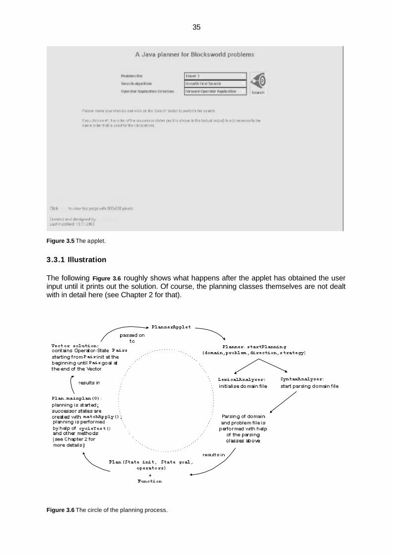
35

Figure 3.5 The applet.

3.3.1 Illustration The following Figure 3.6 roughly shows what happens after the applet has obtained the user input until it prints out the solution. Of course, the planning classes themselves are not dealt with in detail here (see Chapter 2 for that).

Figure 3.6 The circle of the planning process.

36

3.3.2 Output of the Planner After the goal state has been found, the planner chains back from the goal state to the initial state following the “parent link” of each state. Furthermore, all the negative predicates of these states (like (not on-table a)) are eliminated for reading grounds. As the Closed World Assumption (CWA) holds for Blocksworld, this is perfectly permitted. Figure 3.7 shows a typical output of the planner:

Figure 3.7 Output of Solution Path. The first state mentioned here is not associated with an operator, as it is the initial state, which is already given at the beginning. Starting from the second state, operators are included and describe the action that has been taken to transform the preceding state into the subsequent one (operator-state pairs). The applet does not only show the solution path; it also prints out the whole search process at the beginning. If one scrolls up to the top looking at the same example as above, one can see the initial state named as “Current State” (Figure 3.8). During this search process, states are printed out with their negative predicates, too (Figure 3.9). This results from the ADD and DEL operations that are done by the operators during planning. Unfortunately, these accumulate as the search goes on, but they were not removed purposely so that one can follow the process properly. Whenever new successor states are created and added to the search tree, they are printed out, too (Figure 3.8, “Successor Pairs added to the tree”). Sometimes, no successor states are created, which is printed out as “No new Successor Pairs added to the tree.” in Figure 3.8. The planning process stops as soon as the goal state is found. Actually, the process should be stopped as soon as the goal state is created as a successor state, but this is not the case in standard search. The planner does not assess a state until it is chosen as the “current” one. So mostly, a lot of unnecessary states and their successor states are being created if they have been added to the search tree before the goal state, and the search strategy

37

favours these. This is a matter of informed and blind search that is explained in Chapter 2. As a result of the above-mentioned, the output of the search path stops as soon as the goal state is printed out as the current state.

Figure 3.8 New successors are added.

Figure 3.9 Output of “Current State” and “No new successors”.

38

4 Conclusion This chapter mainly summarises the underlying programming work and discusses difficulties and accomplishments.

4.1 Achievements and Problems The aim of this thesis was to describe the fields of problem solving and planning within the scope of Artificial Intelligence, supported by an implementation of a non-linear total-order state-based planner written in an untypical AI language like Java. Concerning the programming, I had different impressions and experiences. The parsing part was fairly easy as I included my inspirations from the Languages and Compilers course at Sussex University (UK) trouble-freely. The planning part was theoretically clear to me, but I had to refine and change my programming concept several times. This was due to choosing Java as a programming language for the planning project. Although I judge myself as fairly advanced in Java, implementing the matching of the operators with the states, remembering which initialisations were already found and which not yet – this was the most demanding part of the project that kept me busy for one full month. Finally, I found a method to tackle this problem, which is described in section 2.3.3. Towards the end of the project I was confronted with a principally unwanted feature of Java, aliasing. Since in Java object references are passed around rather than the objects themselves, this created unpredicted effects in parts of the program where least expected. After completing the programming part successfully, I conclude that planning can be implemented using object-oriented languages like Java, but it is quite complicated and thorny. Many for-clauses, also inner ones are required to simulate matching procedures. Naturally, this slows down the program, but luckily not noticeable enough for Blocksworld problems up to five blocks. Still, classical AI-languages are more suitable for planning indeed – although I do not regret having attempted it with Java. Originally, the applet was intended to include real graphics, i.e. the search tree would have been drawn as solution of the planner instead of the text-based output. I did not master this part by reason of the variable branching factor of Blocksworld. A possible approach is discussed in the next section.

4.2 Outlook Possible future improvements of the program are required in the applet. As mentioned in the previous section, it would be nice if the search tree containing the solution path was drawn on the screen. I attempted this with common Java Swing GUI components, but I had difficulties in drawing the levels properly. This is due to the variable branching factor of the tree, i.e. the nodes can practically possess one to an unlimited number of successor nodes, which complicates the calculation of space allocation for each node. The maximum number of successors of a node has to be known in advance to draw each level properly. Or, some procedure has to remember the location of each node, so that these can be redrawn recursively up to the higher levels once more space is required in the lower ones. On time and experience grounds with Swing, I did not concentrate further on this part.

39

References AIPS-98 Planning Competition Committee (1998). “PDDL – The Planning Domain Definition Language Version 1.2.” http://www.informatik.uni-ulm.de/ki/Edu/Vorlesungen/GdKI/WS0203/ pddl.pdf (16.11.2003). Fox, M., Long, D. (2003). “PDDL2.1: An Extension to PDDL for Expressing Temporal Planning Domains”. http://www.dur.ac.uk/d.p.long/pddl2.ps.gz (16.11.2003). Knoblock, C., A. (1993). “Generating abstraction hierarchies: An Automated Approach to Reducing Search in Planning”. Boston [u.a.]: Kluwer. Marshall, D. (1996). “Artificial Intelligence II” (Script). Cardiff University, UK. http://www.cs.cf.ac.uk/ Dave/AI2/ (16.11.2003). Minton, S. (1993). “Machine learning methods for planning”. San Mateo, California: Kaufmann. Paine, J. (1997). "AI and Problem Solving: Planning". http://www.j-paine.org/students/tutorials/planning/planning.html (03.01.2004). Rich, E., Knight, K. (1991). ”Artificial Intelligence.” New York [et.al.]: McGraw-Hill. Rieksts, O. (2002). “Improving the State Space Search for Blocks World”. Kutztown University, USA. http://faculty.kutztown.edu/rieksts/347/projects/state-search/improve.html (11.09.2003). Russell, S. J., Norvig P. (1995). “Artificial intelligence: A Modern Approach”. Englewood Cliffs, NJ: Prentice Hall. Russell, S. J., Norvig P. (2003). “Artificial intelligence: A Modern Approach”. Upper Saddle River, NJ: Prentice Hall. Schmid, U. (2002). „Denken und Problemlösen -- Computermodelle des Problemlösens“ (Chapt. 5b, 701-734). Contribution to J. Müsseler und W. Prinz (Hrsg.), Lehrbuch Allgemeine Psychologie, Spektrum Verlag. Also available at: http://www.inf.uos.de/schmid/pub-ps/lb-end.pdf (16.11.2003). Schmid, U. (2003). “Inductive Synthesis of Functional Programs -- Learning Domain-Specific Control Rules and Abstract Schemes”. Springer, LNAI 2654. Also available at: http://www.inf.uos.de/schmid/pub-ps/habil.pdf (16.11.2003). Schmidt, C. F. (1996). "Cognition and Computation" (Script). Rutgers University, USA. http://www.rci.rutgers.edu/~cfs/472_html/topics.html (04.01.2004). Simmons, R. (2001). "Planning, Execution & Learning: Linear and Non-linear Planning" (Script). Carnegie Mellon University, USA. http://www-2.cs.cmu.edu/~reids/planning/handouts/Linear.pdf (04.01.2004). Stillings, N. A. et al. (1998). “Cognitive Science: an introduction”. Cambridge: The MIT Press. Sun Microsystems, Inc. (2002). ”API specification for the Java 2 Platform”. Standard Edition, version 1.4.1. http://java.sun.com/j2se/1.4.1/docs/api/ (16.11.2003).

40

Sun Microsystems, Inc. (2003). “The Java Tutorial”. http://java.sun.com/docs/books/tutorial/ (16.11.2003). Vanhornweder, K. (2002). “Blocks World Heuristics“. University of Minnesota Duluth, USA. http://www.d.umn.edu/~kvanhorn/cs2511/discussions/heuristics.html (11.09.2003). Watson, D. (2001). “Languages and Compilers” (Script). Sussex University, UK. Weiss, G. (2000). “Multiagent systems: a modern approach to distributed artificial intelligence”. Cambridge: MIT Press.

41

Appendix

Extension to part 3.2.2 (Syntax Analyser) The common EBNF notation is used for the Figures 3.4 and 3.5 with the following conventions:

- terminal symbols are quoted with " " such as in "a", which stands for the terminal letter a

- non-terminal symbols are formatted in the common way - = is used to define a non-terminal symbol on the left hand side with its description on

the right hand side - . is used to terminate a definition - [] denotes optionality - {} denotes repetition - | denotes the non-exclusive or-symbol in logic

Blocksworld domain file (from Schmid, 2003) (define (domain blocksworld) (:requirements :strips) (:predicates (clear ?x) (on-table ?x) (arm-empty) (holding ?x) (on ?x ?y)) (:action pickup :cost (1) :parameters (?ob) :precondition (and (clear ?ob) (on-table ?ob) (arm-empty)) :effect (and (holding ?ob) (not (clear ?ob)) (not (on-table ?ob)) (not (arm-empty)))) (:action putdown :cost (3) :parameters (?ob) :precondition (holding ?ob) :effect (and (clear ?ob) (arm-empty) (on-table ?ob) (not (holding ?ob)))) (:action stack :cost (1) :parameters (?ob ?underob) :precondition (and (clear ?underob) (holding ?ob)) :effect (and (arm-empty) (clear ?ob) (on ?ob ?underob) (not (clear ?underob)) (not (holding ?ob)))) (:action unstack :cost (4) :parameters (?ob ?underob) :precondition (and (on ?ob ?underob) (clear ?ob) (arm-empty)) :effect (and (holding ?ob) (clear ?underob) (not (on ?ob ?underob)) (not (clear ?ob)) (not (arm-empty)))) )

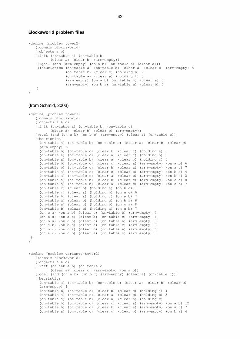
42

Blocksworld problem files (define (problem tower2) (:domain blocksworld) (:objects a b) (:init (on-table a) (on-table b) (clear a) (clear b) (arm-empty)) (:goal (and (arm-empty) (on a b) (on-table b) (clear a))) (:heuristics (on-table a) (on-table b) (clear a) (clear b) (arm-empty) 4 (on-table b) (clear b) (holding a) 2 (on-table a) (clear a) (holding b) 5 (arm-empty) (on a b) (on-table b) (clear a) 0 (arm-empty) (on b a) (on-table a) (clear b) 5 ) ) (from Schmid, 2003) (define (problem tower3) (:domain blocksworld) (:objects a b c) (:init (on-table a) (on-table b) (on-table c) (clear a) (clear b) (clear c) (arm-empty)) (:goal (and (on a b) (on b c) (arm-empty) (clear a) (on-table c))) (:heuristics (on-table a) (on-table b) (on-table c) (clear a) (clear b) (clear c) (arm-empty) 6 (on-table b) (on-table c) (clear b) (clear c) (holding a) 6 (on-table a) (on-table c) (clear a) (clear c) (holding b) 3 (on-table a) (on-table b) (clear a) (clear b) (holding c) 6 (on-table b) (on-table c) (clear c) (clear a) (arm-empty) (on a b) 6 (on-table b) (on-table c) (clear b) (clear a) (arm-empty) (on a c) 7 (on-table a) (on-table c) (clear c) (clear b) (arm-empty) (on b a) 4 (on-table a) (on-table c) (clear a) (clear b) (arm-empty) (on b c) 2 (on-table a) (on-table b) (clear b) (clear c) (arm-empty) (on c a) 8 (on-table a) (on-table b) (clear a) (clear c) (arm-empty) (on c b) 7 (on-table c) (clear b) (holding a) (on b c) 1 (on-table c) (clear a) (holding b) (on a c) 6 (on-table b) (clear a) (holding c) (on a b) 7 (on-table a) (clear b) (holding c) (on b a) 6 (on-table a) (clear c) (holding b) (on c a) 8 (on-table b) (clear c) (holding a) (on c b) 7 (on c a) (on a b) (clear c) (on-table b) (arm-empty) 7 (on b a) (on a c) (clear b) (on-table c) (arm-empty) 6 (on b a) (on c b) (clear c) (on-table a) (arm-empty) 8 (on a b) (on b c) (clear a) (on-table c) (arm-empty) 0 (on b c) (on c a) (clear b) (on-table a) (arm-empty) 6 (on a c) (on c b) (clear a) (on-table b) (arm-empty) 8 ) ) (define (problem variante-tower3) (:domain blocksworld) (:objects a b c) (:init (on-table b) (on-table c) (clear a) (clear c) (arm-empty) (on a b)) (:goal (and (on a b) (on b c) (arm-empty) (clear a) (on-table c))) (:heuristics (on-table a) (on-table b) (on-table c) (clear a) (clear b) (clear c) (arm-empty) 1 (on-table b) (on-table c) (clear b) (clear c) (holding a) 4 (on-table a) (on-table c) (clear a) (clear c) (holding b) 3 (on-table a) (on-table b) (clear a) (clear b) (holding c) 6 (on-table b) (on-table c) (clear c) (clear a) (arm-empty) (on a b) 12 (on-table b) (on-table c) (clear b) (clear a) (arm-empty) (on a c) 7 (on-table a) (on-table c) (clear c) (clear b) (arm-empty) (on b a) 4

43

(on-table a) (on-table c) (clear a) (clear b) (arm-empty) (on b c) 2 (on-table a) (on-table b) (clear b) (clear c) (arm-empty) (on c a) 8 (on-table a) (on-table b) (clear a) (clear c) (arm-empty) (on c b) 7 (on-table c) (clear b) (holding a) (on b c) 1 (on-table c) (clear a) (holding b) (on a c) 6 (on-table b) (clear a) (holding c) (on a b) 8 (on-table a) (clear b) (holding c) (on b a) 6 (on-table a) (clear c) (holding b) (on c a) 8 (on-table b) (clear c) (holding a) (on c b) 7 (on c a) (on a b) (clear c) (on-table b) (arm-empty) 7 (on b a) (on a c) (clear b) (on-table c) (arm-empty) 6 (on b a) (on c b) (clear c) (on-table a) (arm-empty) 8 (on a b) (on b c) (clear a) (on-table c) (arm-empty) 0 (on b c) (on c a) (clear b) (on-table a) (arm-empty) 6 (on a c) (on c b) (clear a) (on-table b) (arm-empty) 8 ) ) (define (problem tower4) (:domain blocksworld) (:objects a b c d) (:init (on-table c) (on-table a) (clear b) (clear c) (on b d) (on d a) (arm-empty)) (:goal (and (arm-empty) (on a b) (on b c) (on c d) (on-table d) (clear a))) )

44

Erklärung Hiermit erkläre ich, Elif Aktolga, die vorliegende Arbeit "A Java planner for Blocksworld problems" selbstständig verfasst zu haben und keine anderen Quellen oder Hilfsmittel als die angegebenen verwendet zu haben. Osnabrück, den 19.01.2004

_______________ Elif Aktolga

Mat.Nr.: 901184