a hybrid particle swarm optimization for parallel machine total tardiness scheduling

ORIGINAL ARTICLE

A hybrid particle swarm optimization for parallel machinetotal tardiness scheduling

Qun Niu & Taijin Zhou & Ling Wang

Received: 15 September 2009 /Accepted: 5 November 2009 /Published online: 28 November 2009# Springer-Verlag London Limited 2009

Abstract The parallel machine scheduling problem hasreceived increasing attention in recent years. This researchconsiders the problem of scheduling jobs on parallelmachines with a total tardiness objective. In the view of itsnon-deterministic polynomial-time hard nature, the particleswarm optimization (PSO), which is inspired by theswarming or collaborative behavior of biological popula-tions, is employed to solve the parallel machine totaltardiness problem (PMTP). Since it is very hard to directlyapply standard PSO to this problem, a new solutionrepresentation is designed based on real number encoding,which can conveniently convert the job sequences of PMTPto continuous position values. Moreover, in order to enhancethe performance of PSO, we introduce clonal selectionalgorithm (CSA) into PSO and therefore propose a newCSPSO method. The incorporation of CSA can greatlyimprove the swarm diversity and avoid premature conver-gence. We further investigate three parameters of PSO andCSPSO, finding that the parameters have marginal impact onCSPSO, which indicates that CSPSO is a very stable androbust method. The performance of CSPSO is evaluated incomparison with traditional genetic algorithm (GA) andstandard PSO on 250 benchmark instances. Experimentalresults show that CSPSO significantly outperforms GA andPSO, with obtaining the optimal solutions of 237 instances.Additionally, PSO appears more effective than GA.

Keywords Parallel machine scheduling . Particle swarmoptimization . Clonal selection algorithm . Total tardiness

1 Introduction

This paper considers an identical parallel machine totaltardiness problem (PMTP). Minimizing total tardiness isone of the most important criteria in many manufacturesystems, especially in the current situation where competi-tion is becoming more and more intensive. Using thestandard three-field classification scheme, the PMTP isusually denoted as Pm==

PTj, where Pm represents

identical parallel machines and the jobs are not con-strained;

PTjdenotes the objective that is used to minimize

the total tardiness. It is non-deterministic polynomial-time(NP) hard in the strong sense even for a single machine (Duand Leung [1]).

The PMTP, like many other scheduling problems, hasreceived wide attention in the literature due to itsapplications in manufacturing. Some exact methods havebeen developed by researchers. Root [2] considered that alljobs have the same due dates and presented a constructivemethod to minimize the total tardiness. Lawler [3]formulated the parallel machine problem as a transportationproblem when the job processing times are identical.Dogramaci [4] presented a dynamic programming algo-rithm to minimize total weighted tardiness. By consideringidentical due dates and processing times, Elmaghraby andParkin [5] used a branch and bound to minimize somepenalty functions of tardiness. Three years later, thismethod was employed again and improved by Barnes andBrennan [6]. Azigzoglu [7] and Yalaoui [8] also developedthe B&B algorithms for the problem. In the most recentresearch, Tanaka and Araki [9] proposed a new branch-and-bound algorithm. In this algorithm, the Lagrangian relax-ation technique is utilized to obtain a tight lower bound.

Since exact methods are mostly limited to special caseslike common due dates and equal processing times, many

Q. Niu (*) : T. Zhou : L. WangShanghai Key Laboratory of Power Station,School of Mechatronic Engineering and Automation,Shanghai University,Shanghai, Chinae-mail: [email protected]

Int J Adv Manuf Technol (2010) 49:723–739DOI 10.1007/s00170-009-2426-8

heuristic methods have been proposed to solve the problem.Based on neighborhood search, Wilkerson and Irwin [10]developed a heuristic method to minimize the meantardiness on a single machine. This method was thenextended by Baker [11] to solve the parallel-machine case.A heuristic method based on list algorithms was designedfor parallel machine problem by Dogramaci and Surkis[12]. Ho and Chang [13] built an assignment rule notedtraffic priority index, which combined the shortest process-ing time and earliest due dates rules using a newmeasurement called traffic congestion ratio. Recently,several other researchers have also introduced differentheuristics for solving similar problems [14, 15].

With the development of evolutionary computing, manymeta-heuristic methods, such as genetic algorithm (GA),simulated annealing (SA), and tabu search (TS), have beenapplied to PMTP. Bean [16] applied GA to the PMTP. Arepresentation technique called random keys was proposedto maintain feasibility from parent to offspring in GA.Rajakumar [17] used GA to solve the parallel machinescheduling problem of the manufacturing system with theobjective of workflow balancing. Recently, Chaudhry andDrake [18] proposed a GA approach to minimize totaltardiness of a set of tasks for identical parallel machines andworker assignment to machines. Koulamas [19] presented apolynomial decomposition heuristic and a hybrid SAheuristic for the problem. Chang Ouk Kim and Hyun JoonShin [20] presented a restricted TS algorithm that schedulesjobs on parallel machines, which have release times anddue dates, and sequence-dependent setup times. Bilge [21]developed a TS approach to solve the PMTP with sequencedependent setups on uniform parallel machines. Anghinolfiand Paolucci [22] proposed a hybrid metaheuristic ap-proach, which integrates several features from TS, SA, andvariable neighborhood search.

Recently, a new developed search technique, particleswarm optimization (PSO) has been proposed by Kennedyand Eberhart [23] for optimization problems. Like GA,PSO is also a population-based stochastic optimizationalgorithm, inspired by the behavior of a bird flock.

Due to the simple concept, easy implementation, andquick convergence, PSO has been widely applied in avariety of optimization problems [24–27]. However, be-cause of the specific algorithmic structure of PSO (updatingof position and velocity of particles in a continuousmanner), few studies have been reported in the area ofPSO for scheduling problems. Therefore, in order to applyPSO to the scheduling problems successfully, severalresearchers extended PSO or designed the encodingschemes, which converted the continuous position valuesinto a discrete job sequence. Tasgetiren et al. [28]developed a PSO for a permutation flow shop sequencingproblem. Liao et al. [29] extended the PSO based on the

discrete version to solve flow shop scheduling problems.An effective hybrid PSO was proposed for permutationflow shop scheduling problem with the limited buffers byLiu et al. [30].

In this paper, we present a continuous PSO for thePMTP. It should be noted that, since the encoding schemeof PMTP is usually represented based on jobs or operations,the standard continuous PSO cannot be applied to PMTPdirectly. Therefore, we design a new solution representationbased on real number encoding, which easily converts thejob sequences to continuous position values. In addition,though there are numerous PSO variants, prematureconvergence when solving complex multimodal problemsis still the main deficiency of PSO. Therefore, we propose ahybrid PSO method by incorporating the clonal selectionalgorithm (CSA), which is called CSPSO. The clonalselection is a population-based evolutionary algorithm,which uses hyper-mutation and re-selection to fulfillthe search task. The incorporation of CSA can improvethe swarm diversity and avoid premature convergence. Theparameter settings of PSO and CSPSO are also investigat-ed. To test the effectiveness of the proposed CSPSO, weconduct experiments with 250 benchmark instances andprovide comparison results with GA and PSO, whichclearly show that the proposed CSPSO significantly out-performs GA and PSO on all test problems.

The rest of this paper is organized as follows. Section 2gives a brief description of the PMTP. The details of thePSO are outlined in Section 3. Section 4 describes the CSA.In Section 5, the framework of CSPSO is given, and theimplementation methodology of the CSPSO on the PMTPis presented. In Section 6, parameter selection is presentedfirst, and then the computational results are reported anddiscussed. This paper ends with conclusions in Section 7.

2 Total tardiness problem on identical parallel machines

Among all types of scheduling objectives, earliness andtardiness are very important. In this section, we will give adescription of total tardiness problem on identical parallelmachines. The problem can be stated as follows: There aren jobs and all of them are to be processed on m identicalparallel machines. All jobs are available to be processed attime zero, and no job preemption is allowed. Each job onlyneeds to be carried out on one of the identical parallelmachines during a fixed processing time without preemp-tion. Each machine can process any job but only one job ata time. The processing time and due date are given inadvance and machines process another job after the formercompleted. The objective of this paper is to sequence alljobs on the machines such that the total tardiness isminimized. Figure 1 shows a schematic diagram of parallel

724 Int J Adv Manuf Technol (2010) 49:723–739

machine scheduling problem with eight jobs and threeidentical parallel machines.

We will use the following notations throughout the restof this paper:

i index of machine, i=1, 2, …,m, m is the total parallelmachine number

p ¼ fs1; s2; :::s j; :::; sk ig the sequence of jobs which areallocated to machine i toprocess

σj index of job, j=1, 2,..., ki, kirepresents the number of thetotal jobs which are processedby parallel machine i

ps j the processing time of job σj

ss j the starting time of job σj

cs j the completion time of job σj

ds jthe due date of job σj

Mathematically, the PMTP can then be represented inthe following manner:

ss1 ¼ 0 ð1Þ

cs1 ¼ ss1 þ ps1 ð2Þ

ss j ¼ cs j�1 ; j > 1 ð3Þ

cs j ¼ ss j þ ps j ; j > 1 ð4Þ

Therefore, the tardiness time of job σj is calculated bythe following Eq. 5.

Ts j ¼ max 0; cs j � ds j

� � ð5ÞThe objective of this paper is to minimize the total

tardiness, which can be defined by Eq. 6.

T ¼Xmi¼1

Xkij¼1

Ts j ð6Þ

3 Particle swarm optimization

The PSO was first introduced by Kennedy and Eberhart[23] in 1995. In PSO, each potential solution is a point inthe search space and may be regarded as a particle. Initially,a bunch of particles are randomly created and set intomotion through the multidimensional problem space. Intheir movement, the particles have memory, and eachparticle adjusts its position based on its own experience aswell as the experience of a neighboring particle by utilizingthe best position encountered by itself and its neighbors.The previous best value is called the pbest of the particle,and the best value of all the particles’ pbest in the swarm iscalled the gbest. In each iteration, the velocity and theposition of each particle will be updated according to itspbest and gbest.

Suppose that the search space has D-dimensional, andthe position of the ith particle at the tth iteration isrepresented by Xt

i ¼ xti1; xti2; :::; x

tid ; :::; x

tiD

� �. The velocity

of the ith particle at the tth iteration is denoted asV ti ¼ vti1; v

ti2; :::; v

tid :::; v

tiD

� �. Pt

li ¼ pti1; pti2; ::::::; p

tiD

� �is the

best position of the ith particle at the tth iteration. The bestposition found for all swarm is denoted as Pt

g ¼ptg1; p

tg2; ::::::; p

tgD

� �at the tth iteration. The velocity and

position of particles are updated by the Eqs. 7 and 8 in thestandard PSO.

vtþ1id ¼ w� vtid þ c1 � randðÞ � ptid � xtid

� �þ c2

� randðÞ � ptgd � xtid

� �ð7Þ

xtþ1id ¼ xtid þ vtþ1

id ð8Þwhere xtid and vtid represent the position and velocity of thedth dimension of the ith particle at the tth iteration,respectively. w is the inertia weight introduced to balancebetween the global and local search abilities, and rand() is arandom number generator with a uniform distribution over[0, 1]. c1 and c2 are the acceleration constants, which

Fig. 1 Schematic diagram of PMSP

Int J Adv Manuf Technol (2010) 49:723–739 725

represent the weighting of stochastic acceleration terms thatpull each particle toward pbest and gbest.

The updating formula leads particles moving towardcompound vector of local and global optimal solutions.Therefore, opportunity for particles to reach the optimalsolution will be increased. Figure 2 shows the searchprocess of a particle from an old position to a new position.

4 Clonal selection algorithm

The CSA is a population-based stochastic algorithm, whichwas designed by De Castro and Von Zuben [31]. CSA isinspired by the clonal selection principle of acquiredimmunity. In the immune system, the antibody representsa solution to the problem, and an antigen denotes theevaluation of the problem space. The general CSA modelincludes the selection of antibodies (candidate solutions)based on affinity either by matching against an antigenpattern or via evaluation of a pattern by a cost function. Theselected antibodies proliferate into several clones in termsof the affinity, i.e., the higher affinity, the higher number ofclones. A subpopulation is constructed with an antibodyand its clones. The antibodies in the subpopulation thenperform high rate hypermutation. The maturated clones arethen evaluated over the affinity function, and the bestantibody of each subpopulation is selected for surviving.Therefore, a maturated antibody population is updated andgenerated.

CSA contains three operations, which are cloning,mutation, and selection. A set of antibodies are selected,

which have the best highest affinity with antigen from theantibodies. The selected antibodies are cloned in proportionto their affinity with the antigen (rank based). All the copiesare mutated. The mutation degree is inversely rated to theirparent’s affinity. All the copies are added to the antibodies.A set of antibodies from all antibodies that have the besthighest affinity with the antigen are re-selected. Figure 3presents the basic state transfer flowchart of CSA.

Since CSA has the advantage of being simple toimplement and easy to understand, it has shown consider-able success in solving a variety of optimization problem[32–34]. CSA also has been reported in scheduling area.For example, Yang [35] proposed a clonal selection-basedmemetic algorithm for solving job shop scheduling prob-lems. Kumar et al. [36] extended the artificial immunesystem approach by proposing a new methodology termedas psycho-clonal algorithm to solve m-machine no-waitflow shop problem.

5 The proposed CSPSO and its implementationto the PMTP

The social and cognitive adaptation makes PSO focus moreon the cooperation among the particles. In the original PSO,all particles in the swarm learn from the gbest even if thecurrent gbest is far from the global optimum, and in thelocal paradigm, particles have information only of theirown and their nearest array neighbors’ bests, rather thanthat of entire group. Meanwhile, particles in the swarm willnever be removed even if they are impossible to reach thebest position, which may waste the limited computationalresources. Therefore, after some generations, the populationdiversity would be greatly reduced, and the PSO might leadto a premature convergence to a local optimum. CSA is apowerful stochastic optimization technique, which hassome distinguished features. The individuals of the popu-lation can be operated in search space simultaneously, andit utilizes probabilistic transition rules instead of determin-istic ones. It also has the ability of getting out local minima.Clearly, the advantage of one algorithm can be the remedyfor the shortcoming of PSO. The incorporation of CSA intoPSO as a local improvement procedure enables thealgorithm to maintain the population diversity and escapefrom local optima.

Based on the complementary properties of PSO andCSA, a hybrid algorithm, called CSPSO, is proposed to

xidt

pgdt

pidt

vidt

vidt+1

xidt+1

x

y Search space

Fig. 2 Search process of standard PSO

pop(t) pop1(t) pop2(t) pop(t+1)

cloning operation mutation operation selection operationFig. 3 Basic state transfer flow-chart of CSA


combine the cooperative and competitive characteristics ofboth PSO and CSA. In other words, the PSO is employedto improve the survival individuals and maintain thediversity in CSA.

Figure 4 shows the framework of the CSPSO for solvingthe PMTP, and as can be seen in this figure, the first half ofthe algorithm, is an ordinary clonal selection operation.After the cloning, mutation, and selection operations, PSOis performed to update the new population and enforce thesearch ability. It should be pointed out that the velocity andposition in CSPSO are updated by the normal PSOoperators. The procedures of CSPSO for solving this PMTPcan be described in Fig. 5.

Next, we describe the detailed implementation of theproposed CSPSO as follows.

5.1 Solution representation

The most important issue in applying CSPSO and PSO tothe PMTP is to design an encoding scheme that allows one-to-one mapping between solutions and structures (par-ticles). There are several types of solution representationfor PTMT. For instance, Kashan [37] adopted a discreteencoding to solve the parallel machine scheduling problem.A solution representation for the problem of assigning jobs

to machines is represented by an array whose length isequal to the number of jobs. The jth gene denotes themachine which the jth job is assigned to. Figure 6a shows asolution representation for the problem with ten jobs andfour machines. Jobs 1, 3, and 5 are processed by machine 1.Machine 2 processes jobs 2 and 10. Jobs 4, 8, and 9 areassigned to machine 3. Machine 4 processes the remainingjobs. Sivirkaya-Şerifoğlu [38] used a chromosome repre-sentation, which incorporated both the job sequencing andthe machine selection dimensions of the problem. Eachgene contains two pieces of information, a job and thenumber of the machine selected for its processing. Anexample of the solution representation is shown in Fig. 6b.Lee [39] utilized the number of jobs to represent a solution.S=(S1, …, Sm) represents a schedule where Sj is the subsetof jobs assigned to machine Mj under S. Figure 6cdemonstrates the solution presentation, which contains foursubsets. The first subset denotes that jobs 3, 1, and 5 are tobe processed on machine 1 in the given order. The secondone represents that jobs 2 and 10 are assigned to machine 2.The third subset shows that jobs 8, 4, and 9 are to beprocessed on machine 3. The last subset indicates that theremaining jobs are processed on the last machine.

In this paper, the above mentioned solution representa-tions are mainly based on job sequences or machine

Define the search space, population size,objective function and let t=0

Initialize position P and velocity V, and define thePl (local best) and Pg (global best)

Perform the clonal seletion operation for thepopulation

Update the velocity and position according toEq.(7) and Eq.(8)

Caculate the objective value for eachparticle and update the Pl and Pg

t=t+1

Stop criteriamet?

Output the bestschedule

YesNo

Fig. 4 Flowchart of CSPSO


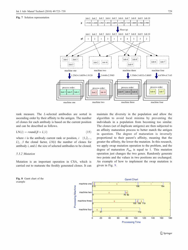
numbers, which cannot be used in PSO. Therefore, wepropose a new encoding method based on the real numberencoding. For a PMTP with n jobs and m parallel machines,we randomly generate n real numbers from a uniformdistribution between [1, m+1). A real number encodingwhose integer part denotes the machine that the job isassigned to and whose fractional part represents theprocessing order of jobs on each machine. Based on thereal number encoding, the sequence of jobs on eachmachine can be converted to continuous position values.We will give an example as follows: ten jobs are processedon four parallel machines. Figure 7 illustrates the solutionrepresentation. Applying this encoding scheme, it isconvenient to know the job number assigned to eachmachine and the process order of jobs processed on thesame machine.

In order to describe the above example more clearly, wegive the Gantt chart, as shown in Fig. 8. Suppose theprocessing time P=[58 76 6 16 100 21 89 13 100 6] and thedue dates D=[19 30 31 24 37 5 29 41 16 54]. Therefore,the total tardiness can be calculated based on Eq. 6, whichis equal to 545.

5.2 Initial population

Each particle has its own position and velocity. Thealgorithm first starts by generating a population P, whichis composed of Np particles. Each individual xi also has D-dimensional parameter vectors. The index t denotes theiteration number of the algorithm. The population P is usedto represent the positions of particle. The initial positionpopulation can be generated randomly by using Eq. 11. mrepresents the number of identical parallel machines, andrand is a random value between 0 and 1.

PðtÞ ¼ x1ðtÞ; x2ðtÞ; . . . ; xiðtÞ; . . . ; xNpðtÞ� � ð9Þ

xiðtÞ ¼ x1;iðtÞ; x2;iðtÞ; . . . ; xj;iðtÞ; . . . ; xD;iðtÞ� � ð10Þ

xj;ið0Þ ¼ randðÞ � mþ 1i ¼ 1; 2; . . . ;Np; j ¼ 1; 2; . . . ;D; t ¼ 1; 2; . . . ; T

ð11ÞA population V, which is composed of Np individuals,

denotes the velocity of each particle. It also has D-dimensional parameter vectors. The initial velocity popula-tion can be generated using Eq. 14. The velocity of eachparticle is equal to zeros. It means that all particles have novelocity in the initial generation.

V ðtÞ ¼ v1ðtÞ; v2ðtÞ; :::; viðtÞ; :::; vNpðtÞ� � ð12Þ

viðtÞ ¼ v1;iðtÞ; v2;iðtÞ; . . . ; vj;iðtÞ; . . . ; vD;iðtÞ� � ð13Þ

V ð0Þ ¼ zeros Np;D� � ð14Þ

5.3 Clonal selection operations

In the following, clonal selection operation involvingcloning operation, mutation operation, and selection oper-ation are described in detail.

5.3.1 Cloning operation

The cloning operation can expand the number of individ-uals that have higher affinities. In this paper, we adopt thetotal tardiness to calculate the affinities, i.e., the smallertotal tardiness (higher affinity), the higher the number ofcopies and vice versa. A set of L antibodies are selected thathave the best highest affinity with antigen from the Kantibodies. The number of clones generated from each of aset of L-selected antibodies is rated to their affinity using a

1 2 3 21 3 1 4 4 3

Job 1 Job 2 Job 3 Job 4 Job 5 Job 6 Job 7 Job 8 Job 9 Job 10

(a)

2-2 8-3 6-4 3-11-1 4-3 10- 2 7-4 5-1 9-3

(b)

(c)machine one machine two machine three machine four

3 1 5 2 10 8 4 9 7 6

Fig. 6 Three types of solution representation

Step 1: Define the search space, population size and objective function.

Step 2: Initialize a swarm of particles with random positions and velocities in the

multi-dimensional scheduling problem space.

Step 3: Define the local best solution lP and the global best solution gP .

Step 4: Perform the clonal selection operation on the population.

Step 5: Update the current positions and velocities of all particles using Eq.(7)

and(8).

Step 6: Calculate the value of the objective function for each particle and update the

current local best and global best.

Step 7: Loop to step (4) until a stop criterion is satisfied, usually a sufficiently good

fitness or a specified number of generations.

Fig. 5 Procedures of CSPSO for solving the PMTP


rank measure. The L-selected antibodies are sorted inascending order by their affinity to the antigen. The numberof clones for each antibody is based on the current positionand can be described as follows.

LNðiÞ ¼ round b � L=ið Þ ð15Þwhere i is the antibody current rank or position, i {1,2,...,L}, β the clonal factor, LN(i) the number of clones forantibody i, and L the size of selected antibodies to be cloned;

5.3.2 Mutation

Mutation is an important operation in CSA, which iscarried out to maturate the freshly generated clones. It can

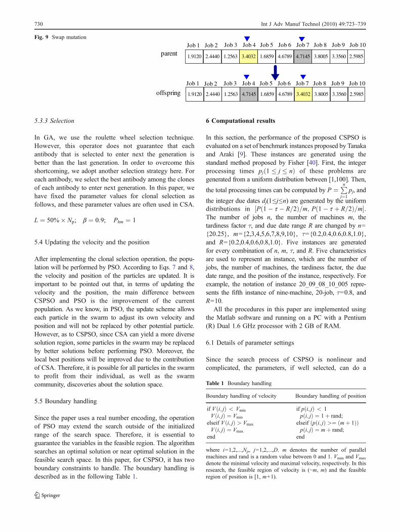
maintain the diversity in the population and allow thealgorithm to avoid local minima by preventing theindividuals in a population from becoming too similar.The clones (set of duplicate antigens) are then subjected toan affinity maturation process to better match the antigenin question. The degree of maturation is inverselyproportional to their parent’s affinity, meaning that thegreater the affinity, the lower the mutation. In this research,we apply swap mutation operation to the problem, and thedegree of maturation Phm is equal to 1. This mutationoperation just changes the two genes. Randomly generatetwo points and the values in two positions are exchanged.An example of how to implement the swap mutation isgiven in Fig. 9.

3.8005 3.3560 2.5985

Job 1 Job 2 Job 3

4.71454.67891.68593.40321.25632.44401.9120

Job 4 Job 5 Job 6 Job 7 Job 8 Job 9 Job 10

Floor (p)

p

3 3 2

Job 1 Job 2 Job 3

4413121

Job 4 Job 5 Job 6 Job 7 Job 8 Job 9 Job 10

p1

machine one machine two machine three machine four

Job 1 Job 3

Job 5Job 2 Job 10

Job 9Job 6 Job 7

1.2563<1.6859<1.9120 2.4440<2.5985 3.3560<3.4032<3.8005 4.6789<4.7145

process order: process order: process order: process order:

Job 3 Job 5 Job 1 Job 2 Job 10 Job 4 Job 8Job 9 Job 6 Job 7

Job 4 Job 8

machine one machine two machine three machine four

Fig. 7 Solution representation

0 20 40 60 80 100 120 140 160 180

machine one

machine two

machine three

machine four

Pro

cess

ing

Mac

hine

Processing Time

Gannt Chart

106 1641

0 762

0 63

1064

5

0 216

1107

1198

09

8210

100

Fig. 8 Gantt chart of theexample


5.3.3 Selection

In GA, we use the roulette wheel selection technique.However, this operator does not guarantee that eachantibody that is selected to enter next the generation isbetter than the last generation. In order to overcome thisshortcoming, we adopt another selection strategy here. Foreach antibody, we select the best antibody among the clonesof each antibody to enter next generation. In this paper, wehave fixed the parameter values for clonal selection asfollows, and these parameter values are often used in CSA.

L ¼ 50%� Np; b ¼ 0:9; Phm ¼ 1

5.4 Updating the velocity and the position

After implementing the clonal selection operation, the popu-lation will be performed by PSO. According to Eqs. 7 and 8,the velocity and position of the particles are updated. It isimportant to be pointed out that, in terms of updating thevelocity and the position, the main difference betweenCSPSO and PSO is the improvement of the currentpopulation. As we know, in PSO, the update scheme allowseach particle in the swarm to adjust its own velocity andposition and will not be replaced by other potential particle.However, as to CSPSO, since CSA can yield a more diversesolution region, some particles in the swarm may be replacedby better solutions before performing PSO. Moreover, thelocal best positions will be improved due to the contributionof CSA. Therefore, it is possible for all particles in the swarmto profit from their individual, as well as the swarmcommunity, discoveries about the solution space.

5.5 Boundary handling

Since the paper uses a real number encoding, the operationof PSO may extend the search outside of the initializedrange of the search space. Therefore, it is essential toguarantee the variables in the feasible region. The algorithmsearches an optimal solution or near optimal solution in thefeasible search space. In this paper, for CSPSO, it has twoboundary constraints to handle. The boundary handling isdescribed as in the following Table 1.

6 Computational results

In this section, the performance of the proposed CSPSO isevaluated on a set of benchmark instances proposed by Tanakaand Araki [9]. These instances are generated using thestandard method proposed by Fisher [40]. First, the integerprocessing times pj 1 � j � nð Þ of these problems aregenerated from a uniform distribution between [1,100]. Then,

the total processing times can be computed by P ¼ Pnj¼1

pj, and

the integer due dates dj(1≤j≤n) are generated by the uniformdistributions in P 1� t � R=2ð Þ=m; P 1� t þ R=2ð Þ=m½ �.The number of jobs n, the number of machines m, thetardiness factor τ, and due date range R are changed by n={20.25}, m={2,3,4,5,6,7,8,9,10}, τ={0.2,0.4,0.6,0.8,1.0},and R={0.2,0.4,0.6,0.8,1.0}. Five instances are generatedfor every combination of n, m, τ, and R. Five characteristicsare used to represent an instance, which are the number ofjobs, the number of machines, the tardiness factor, the duedate range, and the position of the instance, respectively. Forexample, the notation of instance 20_09_08_10_005 repre-sents the fifth instance of nine-machine, 20-job, τ=0.8, andR=10.

All the procedures in this paper are implemented usingthe Matlab software and running on a PC with a Pentium(R) Dual 1.6 GHz processor with 2 GB of RAM.

6.1 Details of parameter settings

Since the search process of CSPSO is nonlinear andcomplicated, the parameters, if well selected, can do a



parent

offspring

3.8005 3.3560 2.59854.71454.67891.68593.40321.25632.44401.9120

3.8005 3.3560 2.59853.40324.67891.68594.71451.25632.44401.9120

Fig. 9 Swap mutation

Table 1 Boundary handling

Boundary handling of velocity Boundary handling of position

if V i; jð Þ < Vmin

V i; jð Þ ¼ Vmin

elseif V i; jð Þ > Vmax

V i; jð Þ ¼ Vmax

end

if p i; jð Þ < 1p i; jð Þ ¼ 1þ rand;

elseif p i; jð Þ >¼ mþ 1ð Þð Þp i; jð Þ ¼ mþ rand;

end

where i=1,2,...,Np, j=1,2,...,D. m denotes the number of parallelmachines and rand is a random value between 0 and 1. Vmin and Vmax

denote the minimal velocity and maximal velocity, respectively. In thisresearch, the feasible region of velocity is (−m, m) and the feasibleregion of position is [1, m+1).


good job. Parameter selection is one of the most importantissues in CSPSO and PSO. In this paper, we mainly studythree parameters of the two algorithms. They are the inertiaweight w and the acceleration constants c1 and c2,respectively. In order to determine the parameter settingsper algorithm that yields the best performance, fivebenchmark instances are tested with the following valuesw {0.1 ,0 .2 ,0 .3 ,0 .4 ,0 .5 ,0 .6 ,0 .7 ,0 .8} and c1 = c2{0.5,1.0,1.5,2.0,2.5,3.0}.

In each experiment, the population size (PS) is set to 20,and the number of generations (G) is set to 200. Ten

independent runs are performed on each case. Tables 2 and3 show the comparison of CSPSO and PSO in terms ofdifferent values of w, c1, and c2, where “Min” denotes thebest solution among ten runs, “Avg” means the averagevalue of the ten runs, and “Max” represents the worst valueamong ten runs. “Opt*” in the tables denotes the optimalsolution of the instance.

From Table 2, it can be observed that the results obtainedby PSO are a little different under different values of w.When w=0.2, the results, especially with respect to theaverage results, are better than others. However, the results

Table 2 Comparison of CSPSO and PSO in terms of different values of w

Method w 20_02_02_02_002 20_04_02_02_002 20_06_02_02_002 20_08_02_02_002 20_10_02_02_002Opt*=102 Opt*=105 Opt*=116 Opt*=123 Opt*=136Min/Avg/Max Min/Avg/Max Min/Avg/Max Min/Avg/Max Min/Avg/Max

CSPSO 0.1 102/102/102 105/105/105 116/116/116 123/124.4/126 136/136.8/137

0.2 102/102/102 105/105/105 116/116/116 123/123.4/126 136/136.6/137

0.3 102/102/102 105/105/105 116/116/116 123/123.7/126 136/136.6/137

0.4 102/102/102 105/105/105 116/116/116 123/124.3/126 136/136.9/137

0.5 102/102/102 105/105/105 116/116/116 123/124.2/126 136/136.9/137

0.6 102/102/102 105/105/105 116/116/116 123/123.7/126 136/136.9/137

0.7 102/102/102 105/105/105 116/116/116 123/123.7/126 136.6/136.6/137

0.8 102/102/102 105/105/105 116/116/116 123/124.1/126 136.6/136.6/137

PSO 0.1 102/102.8/110 105/114.4/125 116/124.2/145 129/136/147 139/151.5/174

0.2 102/102/102 105/108.9/113 116/122.6/130 127/133.4/141 139/147.2/160

0.3 102/102.8/110 105/111.6/116 116/125.6/140 130/137.2/147 139/147.6/176

0.4 102/103.2/110 105/112.1/116 116/124.7/133 129/140.1/155 139/148/162

0.5 102/102.6/106 105/110.7/120 117/124.5/130 130/136/147 139/148.4/163

0.6 102/103.2/110 105/109.9/116 124/132.2/142 130/138/146 138/158.5/181

0.7 102/102.4/106 108/116.8/133 126/134.6/141 134/152.9/168 154/174.1/196

0.8 102/103.2/110 105/116.5/124 123/142.3/162 152/169.3/193 155/196.6/235

Table 3 Comparison of CSPSO and PSO in terms of different values of c1 and c2

Method c1=c2 20_02_02_02_002 20_04_02_02_002 20_06_02_02_002 20_08_02_02_002 20_10_02_02_002Opt*=102 Opt*=105 Opt*=116 Opt*=123 Opt*=136Min/Avg/Max Min/Avg/Max Min/Avg/Max Min/Avg/Max Min/Avg/Max

CSPSO 0.5 102/102/102 105/105/105 116/116/116 123/124.3/126 136/136.7/137

1.0 102/102/102 105/105/105 116/116/116 123/124.6/126 136/136.9/137

1.5 102/102/102 105/105/105 116/116/116 123/123.9/126 136/136.9/137

2.0 102/102/102 105/105/105 116/116/116 123/123.7/126 136/136.6/137

2.5 102/102/102 105/105/105 116/116/116 123/124.1/126 136/136.8/137

3.0 102/102/102 105/105/105 116/116/116 123/125.1/128 136/136.7/137

PSO 0.5 102/110.8/126 122/166.1/212 149/204.2/261 173/219.9/265 195/236.1/277

1.0 102/113.6/152 108/128.4/149 139/160.8/216 156/181.1/244 151/202.2/243

1.5 102/105.7/118 105/113.6/128 122/132.3/155 137/150.2/167 152/178.2/254

2.0 102/102.8/110 105/111.6/116 116/125.6/140 130/137.2/147 139/147.6/176

2.5 102/103.6/110 105/114.5/124 129/139.6/149 143/162.7/179 155/180.6/221

3.0 102/103.4/110 116/123.3/141 138/161.5/193 154/202.5/252 207/240.1/275


produced by CSPSO are very similar. For example, for thethree instances, 20_02_02_02_002, 20_04_02_02_002, and20_06_02_02_002, the results are exactly the same. For theremaining instances, w=0.2 is slightly better than others.

In terms of c1 and c2, the results in Table 3 indicate thatPSO can yield better solutions when c1=c2=2.0, while forCSPSO, like the above parameter w, the comparison is notevident. When c1=c2=2.0, CSPSO can perform a littlebetter. It also can be seen that CSPSO can obtain betterresults than PSO, especially for 20_08_02_02_002 and20_10_02_02_002.

Hence, we can conclude that the three parameters do nothave a significant impact on CSPSO, which indicates thatCSPSO are very stable and robust. In order to calculateconveniently, the three parameters of CSPSO are deter-mined with the same of PSO in the following experiments,i.e., w=0.2, c1=c2=2.0.

6.2 Simulation results on 250 instances

In order to evaluate the performance of CSPSO, 250benchmark instances are selected, whose characteristics

are n=20, m={2,4,6,8,10}, τ={0.2,0.4,0.6,0.8,1.0}, andR={0.2,0.4,0.6,0.8,1.0}, respectively. For the five instancesgenerated for every combination of n, m, τ, and R, we justselect the even number instances.

To verify the validity of CSPSO, experiments are con-ducted to make a comparison with GA and standard PSO. Allthe algorithms run ten times on each instance, with thefollowing settings: PS=20, G=200. For GA, single-pointcrossover operation and swap mutation operation areadopted. The crossover rate and the mutation rate are set to0.8 and 0.1. The worst solution, average solution, and bestsolution found over ten runs are presented for eachalgorithm.

Tables 4, 5, 6, 7, and 8 summarize the comparisonresults obtained by CSPSO, GA, and PSO with differentmachine numbers. Each table consists of 50 instances. It isclear from Tables 4, 5, 6, 7, and 8 that CSPSO significantlyoutperforms GA and PSO in solving all the instances, and itcan obtain 237 optimal solutions out of the 250 instances.Furthermore, we can also observe that even some worstsolutions yielded by CSPSO are better than the bestsolutions obtained by PSO and GA.

Table 4 Comparison of the three algorithms for instances with 20 jobs and 2 parallel machines

Instance no. Opt* CSPSO GA PSOMin/Avg/Max Min/Avg/Max Min/Avg/Max

20_02_02_02_002 102 102/102/102 102/102.4/106 102/102/102

20_02_02_02_004 136 136/136/136 136/149.2/163 136/141.6/150

20_02_02_04_002 17 17/17/17 17/18.1/23 17/17.4/18

20_02_02_04_004 41 41/41.6/42 42/50.9/75 42/54.8/75

20_02_02_06_002 0 0/0/0 0/0/0 0/0/0

20_02_02_06_004 0 0/0/0 0/6.3/27 0/4.8/21

20_02_02_08_002 0 0/0/0 0/0/0 0/0/0

20_02_02_08_004 0 0/0/0 0/2.5/21 0/0.9/9

20_02_02_10_002 0 0/0/0 0/0/0 0/0/0

20_02_02_10_004 0 0/2.2/10 0/25/58 0/20/66

20_02_04_02_002 412 412/412/412 421/427.8/439 412/424.1/438

20_02_04_02_004 564 564/567.2/571 591/606.4/631 569/585.3/603

20_02_04_04_002 254 254/254/254 254/269.3/294 254/262.3/283

20_02_04_04_004 461 461/469.3/481 494/539.6/612 465/521.1/575

20_02_04_06_002 121 121/121/121 121/125.7/134 121/131/161

20_02_04_06_004 381 382/395.1/416 429/459.4/521 400/435/458

20_02_04_08_002 36 36/36/36 36/40.2/62 36/41.7/67

20_02_04_08_004 322 322/341/353 404/451.2/528 351/410.1/465

20_02_04_10_002 0 0/0/0 0/1.3/13 0/2.3/17

20_02_04_10_004 335 335/347.4/361 419/477.7/535 378/449.7/586

20_02_06_02_002 937 937/937/937 954/983.1/1,041 951/969.1/992

20_02_06_02_004 1,216 1,216/1,231.4/1,268 1,278/1,304.3/1,328 1,217/1,270.2/1,313

20_02_06_04_002 739 739/739/739 744/760.4000/778 739/764.8/889

20_02_06_04_004 1,200 1,200/1,211.2/1,219 1,244/1,314/1,428 1,224/1,275.1/1,331

20_02_06_06_002 518 518/527.2/563 542/581/660 529/562.5/608


Table 4 (continued)


20_02_06_06_004 1,201 1,205/1,222.5/1,239 1,344/1,387.6/1,436 1,272/1,309.8/1,356

20_02_06_08_002 328 328/334.1/347 348/380.6/409 346/386.5/451

20_02_06_08_004 1,297 1,297/1,316/1,325 1,349/1,453.4/1,506 1,321/1,380.4/1,447

20_02_06_10_002 137 137/140.9/153 150/179.8/238 153/178/224

20_02_06_10_004 1,091 1,091/1,103.1/1,118 1,184/1,237.8/1,330 1,120/1,160.7/1,231

20_02_08_02_002 1,793 1,793/1,793.1/1,794 1,823/1,852.6/1,881 1,806/1,837.4/1,909

20_02_08_02_004 2,262 2,262/2,272.5/2,274 2,294/2,357.1/2,403 2,276/2,317.7/2,382

20_02_08_04_002 1,557 1,557/1,559.7/1,566 1,603/1,642.3/1,693 1,570/1,617/1,724

20_02_08_04_004 2,324 2,324/2,326.3/2,340 2,406/2,462/2,529 2,347/2,387.4/2,422

20_02_08_06_002 1,193 1,193/1,194.2/1,202 1,225/1,280.6/1,374 1,206/1,241.5/1,315

20_02_08_06_004 2,048 2,048/2,068/2,093 2,132/2,216.3/2,261 2,073/2,126/2,148

20_02_08_08_002 843 843/856.4/873 894/945.2/1,015 868/936.2/1,049

20_02_08_08_004 1,805 1,805/1,815.6/1,832 1,878/1,941.1/2,058 1,841/1,885/1,977

20_02_08_10_002 562 562/577.8/598 593/648.3/751 595/622.6/671

20_02_08_10_004 1,548 1,548/1,559.5/1,574 1,666/1,715.2/1,751 1,589/1,625.4/1,670

20_02_10_02_002 2,862 2,862/2,862.2/2,864 2,912/2,958.4/3,079 2,869/2,893.6/2,929

20_02_10_02_004 3,322 3,322/3,324.2/3,333 3,367/3,434.6/3,518 3,330/3,366/3,388

20_02_10_04_002 2,395 2,395/2,396.4/2,400 2,421/2,485.5/2,541 2,407/2,423.9/2,475

20_02_10_04_004 2,943 2,943/2,943.4/2,947 2,996/3,051.6/3,106 2,949/2,988/3,037

20_02_10_06_002 1,966 1,966/1,970.3/1,974 2,000/2,044.4/2,092 1,980/2,010.4/2,063

20_02_10_06_004 2,618 2,618/2,621.6/2,630 2,664/2,739.2/2,806 2,654/2,675.2/2,718

20_02_10_08_002 1,557 1,557/1,559.3/1,564 1,594/1,634.3/1,667 1,570/1,617/1,699

20_02_10_08_004 2,324 2,324/2,333/2,353 2,432/2,472.1/2,521 2,349/2,382.1/2,425

20_02_10_10_002 1,193 1,193/1,194.7/1,203 1,222/1,287.7/1,399 1,199/1,250.2/1,328

20_02_10_10_004 2,048 2,048/2,068/2,079 2,151/2,196.5/2,272 2,076/2,136.8/2,181

Table 5 Comparison of the three algorithms for instances with 20 jobs and four parallel machines


20_04_02_02_002 105 105/105/105 105/111.8/121 105/108.9/113

20_04_02_02_004 123 123/125.6/134 138/152/173 126/144.4/166

20_04_02_04_002 25 25/25/25 25/37.4/50 30/39.9/50

20_04_02_04_004 51 51/53.7/62 69/98.8/143 65/92.1/155

20_04_02_06_002 0 0/0/0 0/3.7000/21 0/10.3/34

20_04_02_06_004 0 0/4.4/8 24/54.8/88 29/79.40/162

20_04_02_08_002 0 0/0/0 0/0/0 0/0.3/3

20_04_02_08_004 2 2/7/18 24/50.6000/87 2/75.4/112

20_04_02_10_002 0 0/0/0 0/0/0 0/0/0

20_04_02_10_004 33 33/39/46 58/79.2/122 46/82.5/119

20_04_04_02_002 296 296/302.6/304 305/318.2/336 302/315.6/339

20_04_04_02_004 378 379/388.1/392 393/426.9/451 399/421.9/459

20_04_04_04_002 218 218/218/218 222/235.2/256 232/244.6/258

20_04_04_04_004 340 346/356.5/368 375/403.3/440 383/402/419

20_04_04_06_002 129 129/129/129 134/149.2/175 132/159.8/188


In order to compare the search abilities of CSPSO,PSO, and GA, the optimal rate is employed to measurethe performance of the algorithms, which can becalculated by Eq. 16. Figure 10 illustrates the optimalrates achieved by the three algorithms. As it can be seen,94.8% of the total instances can obtain the optimalsolutions using CSPSO, while for PSO and GA, optimalrates are 17.6% and 15.2%, respectively. It is evident thatCSPSO provides superior performance to other algorithmsin the paper, and PSO slightly outperforms GA in terms ofthe number of instances with optimal solutions. Moreover,the detailed comparison between PSO and GA are given in

Table 9. We can find that, although the number of instancesreached optimal solutions is similar between PSO and GA,PSO can get better solutions on 141 instances comparedwith GA. There are only 70 instances where PSO yieldsthe worse solutions than GA. In addition, as for theaverage value, PSO can obtain better values on most ofinstances than GA. Therefore, PSO appears more effectivethan GA.

OP ¼ number of instances reached optimal solutions

total number of the instancesð16Þ

Table 5 (continued)


20_04_04_06_004 314 320/331.5/341 381/409.1/466 365/392.6/433

20_04_04_08_002 50 50/50/50 60/80.4/103 59/83.7/109

20_04_04_08_004 318 322/337.2/349 385/409/444 370/406.2/499

20_04_04_10_002 0 0/0/0 0/16.8/45 0/33.1/64

20_04_04_10_004 367 367/385.2/392 415/455.2494 408/453.6/501

20_04_06_02_002 629 630/630/630 640/665.4/714 664/677.3/717

20_04_06_02_004 789 789/799.7/805 816/843.1/877 815/842.4/873

20_04_06_04_002 503 503/504.8/505 518/546.8/573 513/550.5/580

20_04_06_04_004 793 793/800.3/811 842/871.1/908 828/849.7/886

20_04_06_06_002 389 389/395.5/406 415/446.6/466 413/448.1/510

20_04_06_06_004 829 829/835.6/848 880/922.7/955 861/895.5/934

20_04_06_08_002 310 310/318.1/323 334/362.2/385 356/383.4/471

20_04_06_08_004 866 866/876.9/893 939/967.8/1,005 921/952.4/990

20_04_06_10_002 165 165/169/177 191/228/267 210/240.6/266

20_04_06_10_004 748 749/759/768 839/857.6/881 806/837.7/873

20_04_08_02_002 1,120 1,120/1,121.3/1,123 1,140/1,156.6/1,201 1,139/1,170.3/1,226

20_04_08_02_004 1,370 1,370/1,371.1/1,378 1,393/1,430.7/1,467 1,392/1,414.1/1,474

20_04_08_04_002 1,015 1,015/1,016.5/1,018 1,028/1,059.8/1,111 1,037/1,062/1,100

20_04_08_04_004 1,405 1,405/1,410/1,421 1,449/1,495.5/1,595 1,436/1,472.8/1,514

20_04_08_06_002 807 807/810.4/817 823/868/914 831/847.4/865

20_04_08_06_004 1,276 1,276/1,279.9/1,291 1,318/1,359.7/1,447 1,291/1,333.3/1,375

20_04_08_08_002 636 636/636.7/642 651/682.1/708 662/689.4/746

20_04_08_08_004 1,136 1,136/1,146.6/1,151 1,196/1,222.8/1,247 1,171/1,210.2/1,279

20_04_08_10_002 447 447/456/477 488/520.7/556 489/513/553

20_04_08_10_004 997 997/1,007.9/1,014 1,053/1,105.2/1,141 1,045/1,074.7/1,102

20_04_10_02_002 1,686 1,686/1,686.9/1,689 1,704/1,736.2/1,776 1,705/1,730.4/1,771

20_04_10_02_004 1,930 1,930/1,935.6/1,937 1,974/2,006.4/2,035 1,949/1,973.2/1,987

20_04_10_04_002 1,451 1,451/1,451.6/1,454 1,469/1,497.2/1,555 1,471/1,509.2/1,577

20_04_10_04_004 1,737 1,737/1,738.7/1,754 1,753/1,797/1,838 1,754/1,781.5/1,807

20_04_10_06_002 1,220 1,220/1,220.8/1,221 1,245/1,269.6/1,305 1,225/1,266.4/1,349

20_04_10_06_004 1,564 1,564/1,564.9/1,566 1,613/1,648.7/1,699 1,588/1,607.9/1,647

20_04_10_08_002 1,015 1,015/1,016.4/1,018 1,036/1,063.5/1,086 1,043/1,065.4/1,155

20_04_10_08_004 1,405 1,405/1,409/1,417 1,446/1,496.6/1,549 1,423/1,461.7/1,492

20_04_10_10_002 807 807/807.9/816 824/864.7/913 827/859.8/941

20_04_10_10_004 1,276 1,276/1,281.3/1,294 1,324/1,359/1,384 1,298/1,329.8/1,365


7 Conclusion

In this paper, a hybrid CSPSO is proposed to solve thePMTP. In order to apply PSO to PMTP successfully, wedesign a new solution representation based on real numberencoding, which can convert the job sequences to continuousposition values. To enhance the performance of PSO, we

introduce the CSA into PSO and present the framework ofCSPSO. The incorporation of CSA can improve the swarmdiversity and avoid premature convergence. In addition, weinvestigate three parameters of PSO and CSPSO and findthat, although the three parameters will affect the perfor-mance of PSO, they have little impact on CSPSO. Hence,CSPSO is more stable and robust than PSO.

Table 6 Comparison of the three algorithms for instances with 20 jobs and six parallel machines


20_06_02_02_002 116 116/116/116 116/124.8/136 116/122.6/130

20_06_02_02_004 132 132/135/142 150/162.9/187 153/163.2/180

20_06_02_04_002 41 41/41/41 45/62.4/87 54/68.8/87

20_06_02_04_004 72 72/75.5/81 90/119.7/149 94/127/163

20_06_02_06_002 0 0/0.1/1 0/17.5/39 5/22.8/64

20_06_02_06_004 18 18/24.9/35 50/76.5/105 64/105.6/160

20_06_02_08_002 0 0/0/0 0/0.5/2 0/5.2/21

20_06_02_08_004 20 20/28.3/41 53/81.8/107 56/96.8/140

20_06_02_10_002 0 0/0/0 0/0/0 0/6.2/29

20_06_02_10_004 75 75/77.6/88 100/133.4/168 97/155.2/199

20_06_04_02_002 302 302/302/302 303/314.9/329 302/313.8/327

20_06_04_02_004 363 363/367.1/370 374/390.7/417 370/388.4/410

20_06_04_04_002 227 227/227/227 238/244.9/261 230/241.9/263

20_06_04_04_004 324 324/334.8/350 360/385.8/412 352/380.9/407

20_06_04_06_002 157 157/157/157 157/177.9/200 158/185.7/211

20_06_04_06_004 338 338/346.9/354 374/396.4/409 362/394.2/430

20_06_04_08_002 84 84/84/84 84/114.1/133 89/118.4/147

20_06_04_08_004 363 363/367.8/378 388/422.1/463 395/430.6/483

20_06_04_10_002 20 20/24.7/31 37/61/80 61/79.7/131

20_06_04_10_004 383 383/388.3/400 423/458.5/502 414/451.3/515

20_06_06_02_002 517 517/520.9/527 541/559.3/600 537/564.5/587

20_06_06_02_004 660 660/665.1/668 682/708.1/755 671/695.3/719

20_06_06_04_002 467 467/469.8/474 486/507/522 486/512.8/535

20_06_06_04_004 680 680/687.4/698 711/732/763 714/741.4/790

20_06_06_06_002 412 412/412/412 418/445.1/475 426/449.3/484

20_06_06_06_004 718 718/722.3/729 744/765.3/799 743/764.1/788

20_06_06_08_002 343 343/347.3/355 358/384.7/425 366/387.5/424

20_06_06_08_004 753 753/757.1/765 789/816.4/843 770/795.3/820

20_06_06_10_002 241 241/242.7/251 278/301.2/339 262/296.6/346

20_06_06_10_004 662 666/674.3/679 715/744.9/768 688/724.3/777

20_06_08_02_002 913 913/913/913 913/956/991 914/935/952

20_06_08_02_004 1,090 1,090/1,093.1/1,097 1,098/1,114.8/1,139 1,109/1,123/1,147

20_06_08_04_002 841 841/841.6/842 858/887.1/917 842/882/917

20_06_08_04_004 1,126 1,126/1,126.4/1,138 1,141/1,169.7/1,210 1,147/1,182.2/1,237

20_06_08_06_002 696 696/696.8/699 721/750.6/803 714/748.6/780

20_06_08_06_004 1,024 1,024/1,025.7/1,030 1,044/1,077.7/1,141 1,051/1,069.5/1,097

20_06_08_08_002 564 564/567/570 588/618.7/662 587/624/660

20_06_08_08_004 920 920/922.5/928 955/978.9/1,011 954/973.9/1,007

20_06_08_10_002 451 451/453.8/461 476/495.5/523 475/502.7/527

20_06_08_10_004 850 850/854.8/859 881/906/934 871/905.7/928


Table 6 (continued)


20_06_10_02_002 1,306 1,306/1,310.3/1,316 1,320/1,358.4/1,393 1,316/1,353.3/1,389

20_06_10_02_004 1,486 1,486/1,495.9/1,510 1,507/1,534.5/1,572 1,487/1,519.1/1,592

20_06_10_04_002 1,136 1,136/1,138.6/1,150 1,163/1,190.7/1,218 1,143/1,183.1/1,215

20_06_10_04_004 1,346 1,346/1,346.1/1,347 1,352/1,392/1,425 1,356/1,376.2/1,423

20_06_10_06_002 993 993/993/993 1,014/1,043.8/1,068 993/1,023/1,056

20_06_10_06_004 1,230 1,230/1,233.8/1,237 1,251/1,274.7/1,315 1,246/1,265.7/1,284

20_06_10_08_002 841 841/841.8/842 865/887.9/941 865/897.4/938

20_06_10_08_004 1,126 1,126/1,126.5/1,128 1,158/1,177.2/1,212 1,143/1,172.5/1,225

20_06_10_10_002 696 696/697.4/699 700/730.4/757 713/742.7/784

20_06_10_10_004 1,024 1,024/1,025.2/1,032 1,047/1,081.6/1,118 1,030/1,059.1/1,082

Table 7 Comparison of the three algorithms for instances with 20 jobs and eight parallel machines


20_08_02_02_002 122 123/123.4/126 128/136.5/146 127/133.4/141

20_08_02_02_004 157 157/158.2/161 174/185.4/204 167/179.2/190

20_08_02_04_002 56 56/61.5/66 65/98.6/126 65/93.5/110

20_08_02_04_004 118 118/119.6/123 138/160.1/177 139/162.4/192

20_08_02_06_002 4 4/10.2/16 14/48.2/69 38/60.5/104

20_08_02_06_004 96 96/98.5/105 128/156.5/211 117/157.3/178

20_08_02_08_002 0 0/0/0 3/21.7/45 6/26.5/55

20_08_02_08_004 108 108/112.5/117 139/162/212 154/180.1/234

20_08_02_10_002 2 2/2/2 2/5.3/12 2/20.4/53

20_08_02_10_004 141 141/148.8/161 169/205.8/235 188/225.4/256

20_08_04_02_002 317 317/317/317 317/327.6/340 317/323.5/334

20_08_04_02_004 385 385/385.2/387 387/395.4/404 389/396.4/404

20_08_04_04_002 267 267/267/267 267/277.1/292 267/277.1/295

20_08_04_04_004 383 383/388.5/391 397/413/430 390/408.8/427

20_08_04_06_002 204 204/204.9/205 205/221.6/243 207/225.3/238

20_08_04_06_004 391 391/392.4/396 404/431/462 416/433.9/447

20_08_04_08_002 147 147/148.6/149 149/172/200 149/172.1/202

20_08_04_08_004 395 395/401/408 433/458.6/483 414/438.5/469

20_08_04_10_002 97 97/98.1/100 108/129.7/143 110/140.6/161

20_08_04_10_004 409 409/413.5/420 439/468.7/509 413/450.9/482

20_08_06_02_002 526 526/526/526 526/540.4/564 529/543.1/570

20_08_06_02_004 635 635/635/635 635/658/679 643/662.1/686

20_08_06_04_002 475 475/475/475 475/495.3/533 475/496.2/509

20_08_06_04_004 667 667/667/667 678/690.2/713 668/682.3/695

20_08_06_06_002 422 422/422/422 429/447.7/468 422/446.9/482

20_08_06_06_004 686 686/691.6/694 694/708.5/725 693/714.9/739

20_08_06_08_002 387 387/387/387 404/420.5/451 407/425.5/452

20_08_06_08_004 722 722/723.3/735 748/768.5/782 740/756.7/789

20_08_06_10_002 300 300/300/300 301/320/342 301/327.3/354

20_08_06_10_004 654 654/657.7/665 676/695/720 666/690.3/713


Table 7 (continued)


20_08_08_02_002 803 803/808.5/825 808/843.3/881 820/828.8/846

20_08_08_02_004 931 931/931.8/933 947/983.6/1,029 936/970/986

20_08_08_04_002 763 763/769/785 774/812.6/840 766/805/842

20_08_08_04_004 962 962/964.6/985 1,002/1,021.6/1,048 966/1,005.7/1,068

.20_08_08_06_002 661 661/661.7/668 671/695.2/709 668/689.1/701

20_08_08_06_004 900 900/900.6/904 924/960.3/1,000 928/950.6000/973

20_08_08_08_002 560 560/560.5/565 578/598.9/636 578/601/637

20_08_08_08_004 850 850/850.2/852 855/893.2/963 852/871.7/896

20_08_08_10_002 467 467/467/467 485/502.8/529 482/504.5/531

20_08_08_10_004 783 783/788.6/790 792/819/842 790/814.9/839

20_08_10_02_002 1,128 1,128/1,129.7/1,137 1,140/1,172/1,262 1,141/1,158/1,181

20_08_10_02_004 1,259 1,259/1,264.6/1,287 1,270/1,286.3/1,306 1,272/1,295.4/1,335

20_08_10_04_002 998 998/999.5/1,001 1,009/1,043/1,096 1,001/1,032.1/1,064

20_08_10_04_004 1,154 1,154/1,157.2/1,165 1,160/1,193/1,237 1,179/1,195.1/1,225

20_08_10_06_002 876 876/882.7/895 886/907/921 881/907.3/938

20_08_10_06_004 1,055 1,055/1,059.6/1,075 1,072/1,098.5/1,136 1,064/1,101.8/1,150

20_08_10_08_002 763 763/768.7/782 774/802.2/835 775/795.1/821

20_08_10_08_004 962 962/964.4/986 997/1,018.5/1,047 987/1,006.4/1,024

20_08_10_10_002 661 661/661/661 675/697.8/730 668/698/739

20_08_10_10_004 900 900/900.9/905 919/945.7/989 902/935/972

Table 8 Comparison of the three algorithms for instances with 20 jobs and ten parallel machines


20_10_02_02_002 135 136/136.6/137 137/145.1/154 139/146.3/159

20_10_02_02_004 180 180/180/180 193/203.7/213 188/196.8/209

20_10_02_04_002 85 85/86.5/88 93/112.6/137 88/105.6/122

20_10_02_04_004 162 162/165.8/172 182/203.5/232 168/195.4/213

20_10_02_06_002 35 35/36.7/43 44/65.1/80 49/72.5/91

20_10_02_06_004 157 157/159.4/167 187/207.5/237 184/215.1/248

20_10_02_08_002 24 24/24.3/26 33/44.7/67 40/54.3/80

20_10_02_08_004 164 164/169.6/176 191/225/256 179/209/227

20_10_02_10_002 26 26/26/26 34/47/80 28/43.6/59

20_10_02_10_004 201 201/206.6/213 228/254.4/280 218/256.6/295

20_10_04_02_002 329 329/329.9/330 330/336.6/345 332/339.7/356

20_10_04_02_004 400 400/400/400 404/410.6/422 400/410.2/426

20_10_04_04_002 274 274/276.7/277 277/293.6/358 281/290.7/302

20_10_04_04_004 401 401/401.3/402 407/415.9/429 408/416.4/424

20_10_04_06_002 228 228/230.5/231 231/252.6/306 231/251.7/265

20_10_04_06_004 414 414/415.1/417 433/448.6/469 419/434.4/489

20_10_04_08_002 190 190/192.1/193 193/214/235 210/217.8/230

20_10_04_08_004 424 424/424.7/426 444/469.2/512 439/458.1/489

20_10_04_10_002 136 136/138.3/139 140/171.2/211 150/181.8/243

20_10_04_10_004 436 436/437.9/444 458/489.9/553 453/482/519

20_10_06_02_002 531 531/531/531 532/557/602 531/542.4/558


The performance of CSPSO is evaluated in comparisonwith well-known GA and standard PSO for 250 benchmarkinstances taken from the literature. The results clearlyconfirmed that CSPSO substantially outperforms GA andPSO for all the instances. CSPSO can obtain the optimalsolutions of 237 instances. Moreover, the optimal rate ofCSPSO is 94.8%, while for PSO and GA, they are 17.6%

Table 8 (continued)


20_10_06_02_004 619 619/619/619 619/629.3/660 619/640.7/658

20_10_06_04_002 488 488/488/488 488/502.5/548 488/502.9/518

20_10_06_04_004 640 640/640/640 645/661.7/707 640/649.9/668

20_10_06_06_002 449 449/449/449 449/465/509 455/466.2/487

20_10_06_06_004 657 657/658.4/664 664/684.8/736 669/677.4/693

20_10_06_08_002 412 412/412.7/415 416/429.6/441 416/433.7/472

20_10_06_08_004 684 684/684/684 697/725.2/759 691/710.6/732

20_10_06_10_002 335 335/336.7/339 338/352.6/388 341/357.2/382

20_10_06_10_004 632 632/633/634 648/664.1/687 641/658.9/678

20_10_08_02_002 776 776/776/776 776/808.6/859 776/803.1/833

20_10_08_02_004 865 865/872.9/888 875/912.2/956 865/905.4/944

20_10_08_04_002 742 742/742.2/743 752/771.5/840 742/762.1/794

20_10_08_04_004 891 891/897/907 903/920.9/933 891/922.3/971

20_10_08_06_002 658 658/658.2/660 658/680.4/735 658/676/692

20_10_08_06_004 844 844/844.2/845 847/868.1/905 860/882.9/909

20_10_08_08_002 570 570/570/570 577/595.8/644 575/593.5/621

20_10_08_08_004 793 793/793/793 803/823.7/855 800/815.2/855

20_10_08_10_002 493 493/493/493 499/512.4/554 493/507.3/526

20_10_08_10_004 739 739/740.8/745 745/764.9/786 741/765.1/783

20_10_10_02_002 1,028 1,031/1,038/1,045 1,040/1,058.1/1,086 1,038/1,051.1/1,079

20_10_10_02_004 1,123 1,123/1,144.4/1,158 1,136/1,162.4/1,184 1,123/1,154.1/1,194

20_10_10_04_002 931 931/936.9/943 931/964.9/1,019 938/956.7/989

20_10_10_04_004 1,038 1,043/1,052.1/1,056 1,060/1,094.2/1,146 1,045/1,078.7/1,104

20_10_10_06_002 832 832/832.7/839 838/862/899 837/850.3/888

20_10_10_06_004 958 958/968.5/983 982/998.3/1,020 970/1,000/1,046

20_10_10_08_002 742 742/742/742 742/768/803 742/760.6/805

20_10_10_08_004 891 891/894.4/900 907/944.2/1,007 891/917.1/949

20_10_10_10_002 658 658/658.9/667 658/677.4/708 668/677.3/729

20_10_10_10_004 844 844/844.1/845 847/877.1/918 844/867.4/892

0

0.1

0.2

0.3

0.4

0.5

0.6

0.7

0.8

0.9

1

250 Instances

Opt

imal

Rat

e

CSPSOPSOGA

94.8%

15.2%17.6%

Fig. 10 Optimal rates of CSPSO, PSO, and GA

Table 9 Comparison of the PSO and GA for 250 instances

The number ofinstances

20_02 20_04 20_06 20_08 20_10 Total

PSO (better) GA 34 28 26 24 29 141

PSO (same) GA 14 5 5 8 9 39

PSO (worse) GA 2 17 19 18 14 70


and 15.2%, respectively. Therefore, the proposed CSPSO isboth effective and efficient for the PMTP. Additionally, wefurther compared PSO and GA. The results indicated thatPSO performs better than GA.

In the scope of future work, a further interesting issuethat deserves investigation is extending CSPSO to morecomplex scheduling problems such as job shop scheduling.

Acknowledgments This work is supported by the National NaturalScience Foundation of China (grant no. 60804052), ShanghaiUniversity “11th Five-Year Plan” 211 Construction Project, ChenGuang Plan (2008CG48), Innovative Foundation of Shanghai Uni-versity, and Scientific Research Special Fund of Shanghai ExcellentYoung Teachers. Additionally, the authors would like to thank Mr.Jian Chen for his helpful suggestions.

References

1. Du J, Leung JYT (1990) Minimizing total tardiness on onemachine is NP-hard. Math Oper Res 15(3):483–495

2. Root JG (1965) Scheduling with deadlines and loss function on Kparallel machines. Manag Sci 11(3):460–475

3. Lawler EL (1977) A “pseudopolynomial” algorithm for sequencingjobs to minimize total tardiness. Ann Discrete Math 1:331–342

4. Dogramaci A (1984) Production scheduling of independent jobson parallel identical machines. Int J Prod Res 16:535–548

5. Elmaghraby SE, Park SH (1974) Scheduling jobs on a. number ofidentical machines. AIIE Trans 6:1–13

6. Barnes JW, Brennan JJ (1977) An improved algorithm forscheduling jobs on identical machines. AIIE Trans 9(1):23–31

7. Azigzoglu M, Kirca O (1998) Tardiness minimization on parallelmachines. Int J Prod Econ 55(2):163–168

8. Yalaoui F, Chu C (2002) Parallel machine scheduling to minimizetotal tardiness. Int J Prod Eco 76(3):265–279

9. Tanaka S, Araki M (2008) A branch-and-bound algorithm withLagrangian relaxation to minimize total tardiness on identicalparallel machines. Int J Prod Eco 113(1):446–458

10. Wilkerson LJ, Irwin JD (1971) An improved algorithm forscheduling independent tasks. AIIE Trans 3:245–293

11. Baker KR, Scudder GD (1990) Sequencing with earliness andtardiness penalties: a review. Oper Res 38(1):22–36

12. Dogramaci A, Surkis I (1979) Evaluation of a heuristic forscheduling independent jobs on parallel identical processors.Manag Sci 25(12):1208–1216

13. Ho JC, Chang YL (1991) Heuristics for minimizing meantardiness for parallel machine. Nav Res Logist 38(3):367–381

14. Simon D, Andrew W (2005) Heuristic methods for the identicalparallel machine flowtime problem with set-up times. ComputOper Res 32(9):2479–2491

15. Patrizia B, Gianpaolo G, Antonio G, Emanuela G (2008) Rolling-horizon and fix-and-relax heuristics for the parallel machine lot-sizing and scheduling problem with sequence-dependent set-upcosts. Comput Oper Res 35(11):3644–3656

16. Bean JC (1994) Genetic algorithms and random keys forsequencing and optimization. ORSA J Comput 6(2):154–160

17. Rajakumar S, Arunachalam VP, Selladurai V (2007) Workflowbalancing in parallel machines through genetic Algorithm. Int JAdv Manuf Technol 33(11–12):1212–1221

18. Chaudhry IA, Drake PR (2009) Minimizing total tardiness for themachine scheduling and worker assignment problems in identicalparallel machines using genetic algorithms. Int J Adv ManufTechnol 42(5–6):581–594

19. Koulamas C (1997) Decomposition and hybrid simulated anneal-ing heuristics for the parallel machine total tardiness problem. NavRes Logist 44(1):109–125

20. Kim CO, Shin HJ (2003) Scheduling jobs on parallel machines: arestricted tabu search approach. Int J Adv Manuf Technol 22(3–4):278–287

21. Bilge Ü, Kiraç F, Kurtulan M, Pekgün P (2004) A tabu searchalgorithm for parallel machine total tardiness problem. ComputOper Res 31(3):397–414

22. Anghinolfi D, Paolucci M (2007) Parallel machine total tardinessscheduling with a new hybrid. metaheuristic approach. ComputOper Res 34(11):3471–3490

23. Kennedy J, Eberhart RC (1995) Particle swarm optimization. In:Proc IEEE Int Conf Neural Networks, Piscataway, NJ, USA, pp.1942–1948

24. Ourique CO, Biscaia EC, Pinto JC (2002) The use of particleswarm optimization for dynamic analysis in chemical processes.Comput Chem Eng 26(12):1783–1793

25. Meissner M, Schmuker M, Schneider G (2006) Optimized particleswarm optimization (OPSO) and its application to artificial neuralnetwork training. BMC Bioinformatics 17(1):125–136

26. Thakshila W, Sudharman KJ (2008) Optimal power scheduling forcorrelated data fusion in wireless sensor networks via constrainedPSO. IEEE Trans Wir Comm 7(9):3608–3618

27. Shubham A, Yogesh D, Tiwari MK, Son YJ (2008) Interactiveparticle swarm: a pareto adaptive metaheuristic to multiobjectiveoptimization. IEEE Trans Sys Man Cyber Part A 38(2):258–277

28. Tasgetiren MF, Liang YC, Sevkli M, Gencyilmaz G (2007) Aparticle swarm optimization algorithm for makespan and totalflowtime minimization in permutation flowshop sequencingproblem. Eur J Oper Res 177(3):1930–1947

29. Liao CJ, Tseng CT, Luarn P (2007) A discrete version of particleswarm optimization for flowshop scheduling problems. ComputOper Res 34(10):3099–3111

30. Liu B, Wang L, Jin YH (2008) An effective hybrid PSO-basedalgorithm for flow shop scheduling with limited buffers. ComputOper Res 35(9):2791–2806

31. De Castro LN, Von Zuben FJ (2002) Learning and optimizationusing the clonal selection principle. IEEE Trans Evol Comput 6(3):239–251

32. Gao SC, HW DAI, YANG G, Tang Z (2007) A novel clonalselection algorithm and its application to traveling salesmanproblem. IEICE Trans Fund 90(10):2318–2325

33. Campelo F, Guimaraes FG, Igarashi H, Ramirez JA (2005) Aclonal selection algorithm for optimization in electromagnetics.IEEE Trans Magn 41(5):1736–1739

34. Das S, Natarajan B, Stevens D, Koduru P (2008) Multi-objectiveand constrained optimization for DS-CDMA code design based onthe clonal selection principle. Appl Soft Comput 8(1):788–797

35. Yang JH, Sun L, Lee HP, Qian Y, Liang YC (2008) Clonalselection based memetic algorithm for job shop schedulingproblems. J Bionic Eng 5(2):111–119

36. Kumar A, Prakash A, Shankar R, Tiwari MK (2006) Psycho-Clonal algorithm based approach to solve continuous flow shopscheduling problem. Expert Syst Appl 31(3):504–514

37. Kashan AH, Karimi B (2009) A discrete particle swarmoptimization algorithm for scheduling parallel machines. ComputInd Eng 56(1):216–223

38. Sivrikaya Serifoglu F, Ulusoy G (1999) Parallel machinescheduling with earliness and tardiness penalties. Comput OperRes 26(8):773–787

39. Lee WC, Wu CC, Chen P (2006) A simulated annealing approachto makespan minimization on identical parallel machines. Int JAdv Manuf Technol 31(3–4):328–334

40. Fisher ML (1976) A dual algorithm for the one-machinescheduling problem. Math Program 11:229–251


a hybrid particle swarm optimization for parallel machine total tardiness scheduling

Documents