Permission to make digital or hard copies of part or all of this work for personal or classroom use is granted without fee provided that copies are not made or distributed for commercial advantage and that copies bear this notice and the full citation on the first page. Copyrights for components of this work owned by others than ACM must be honored. Abstracting with credit is permitted. To copy otherwise, to republish, to post on servers, or to redistribute to lists, requires prior specific permission and/or a fee. Request permissions from permissions@acm.org. SCA 2013, July 19 – 21, 2013, Anaheim, California. Copyright © ACM 978-1-4503-2132-7/13/07 $15.00

A Hybrid Lagrangian-Eulerian Formulation for Bubble Generation and Dynamics

Saket Patkar∗

Stanford UniversityMridul Aanjaneya∗

Stanford UniversityDmitriy Karpman∗

Stanford UniversityRonald Fedkiw∗

Stanford UniversityIndustrial Light + Magic

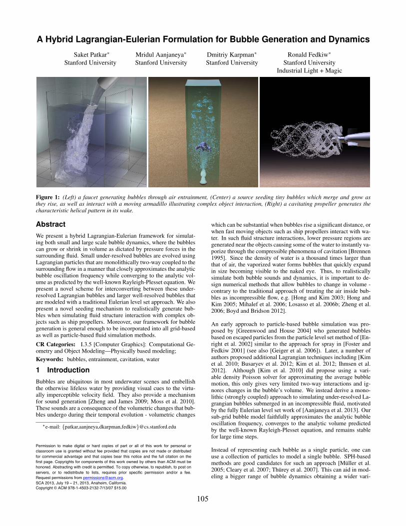
Figure 1: (Left) a faucet generating bubbles through air entrainment, (Center) a source seeding tiny bubbles which merge and grow asthey rise, as well as interact with a moving armadillo illustrating complex object interaction, (Right) a cavitating propeller generates thecharacteristic helical pattern in its wake.

AbstractWe present a hybrid Lagrangian-Eulerian framework for simulat-ing both small and large scale bubble dynamics, where the bubblescan grow or shrink in volume as dictated by pressure forces in thesurrounding fluid. Small under-resolved bubbles are evolved usingLagrangian particles that are monolithically two-way coupled to thesurrounding flow in a manner that closely approximates the analyticbubble oscillation frequency while converging to the analytic vol-ume as predicted by the well-known Rayleigh-Plesset equation. Wepresent a novel scheme for interconverting between these under-resolved Lagrangian bubbles and larger well-resolved bubbles thatare modeled with a traditional Eulerian level set approach. We alsopresent a novel seeding mechanism to realistically generate bub-bles when simulating fluid structure interaction with complex ob-jects such as ship propellers. Moreover, our framework for bubblegeneration is general enough to be incorporated into all grid-basedas well as particle-based fluid simulation methods.

CR Categories: I.3.5 [Computer Graphics]: Computational Ge-ometry and Object Modeling—Physically based modeling;Keywords: bubbles, entrainment, cavitation, water

1 IntroductionBubbles are ubiquitous in most underwater scenes and embellishthe otherwise lifeless water by providing visual cues to the virtu-ally imperceptible velocity field. They also provide a mechanismfor sound generation [Zheng and James 2009; Moss et al. 2010].These sounds are a consequence of the volumetric changes that bub-bles undergo during their temporal evolution - volumetric changes

∗e-mail: patkar,aanjneya,dkarpman,fedkiw@cs.stanford.edu

which can be substantial when bubbles rise a significant distance, orwhen fast moving objects such as ship propellers interact with wa-ter. In such fluid structure interactions, lower pressure regions aregenerated near the objects causing some of the water to instantly va-porize through the compressible phenomena of cavitation [Brennen1995]. Since the density of water is a thousand times larger thanthat of air, the vaporized water forms bubbles that quickly expandin size becoming visible to the naked eye. Thus, to realisticallysimulate both bubble sounds and dynamics, it is important to de-sign numerical methods that allow bubbles to change in volume -contrary to the traditional approach of treating the air inside bub-bles as incompressible flow, e.g. [Hong and Kim 2003; Hong andKim 2005; Mihalef et al. 2006; Losasso et al. 2006b; Zheng et al.2006; Boyd and Bridson 2012].

An early approach to particle-based bubble simulation was pro-posed by [Greenwood and House 2004] who generated bubblesbased on escaped particles from the particle level set method of [En-right et al. 2002] similar to the approach for spray in [Foster andFedkiw 2001] (see also [Geiger et al. 2006]). Later, a number ofauthors proposed additional Lagrangian techniques including [Kimet al. 2010; Busaryev et al. 2012; Kim et al. 2012; Ihmsen et al.2012]. Although [Kim et al. 2010] did propose using a vari-able density Poisson solver for approximating the average bubblemotion, this only gives very limited two-way interactions and ig-nores changes in the bubble’s volume. We instead derive a mono-lithic (strongly coupled) approach to simulating under-resolved La-grangian bubbles submerged in an incompressible fluid, motivatedby the fully Eulerian level set work of [Aanjaneya et al. 2013]. Oursub-grid bubble model faithfully approximates the analytic bubbleoscillation frequency, converges to the analytic volume predictedby the well-known Rayleigh-Plesset equation, and remains stablefor large time steps.

Instead of representing each bubble as a single particle, one canuse a collection of particles to model a single bubble. SPH-basedmethods are good candidates for such an approach [Muller et al.2005; Cleary et al. 2007; Thurey et al. 2007]. This can aid in mod-eling a bigger range of bubble dynamics obtaining a wider vari-

105

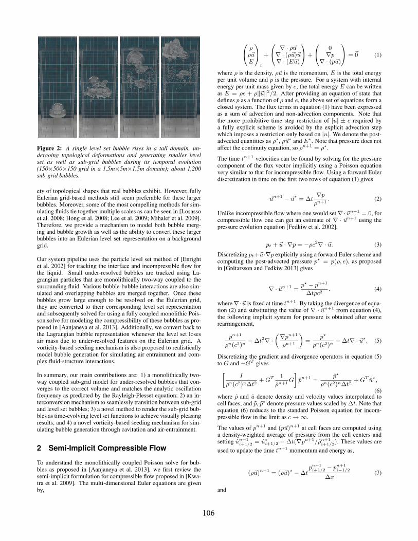
Figure 2: A single level set bubble rises in a tall domain, un-dergoing topological deformations and generating smaller levelset as well as sub-grid bubbles during its temporal evolution(150×500×150 grid in a 1.5m×5m×1.5m domain); about 1,200sub-grid bubbles.

ety of topological shapes that real bubbles exhibit. However, fullyEulerian grid-based methods still seem preferable for these largerbubbles. Moreover, some of the most compelling methods for sim-ulating fluids tie together multiple scales as can be seen in [Losassoet al. 2008; Hong et al. 2008; Lee et al. 2009; Mihalef et al. 2009].Therefore, we provide a mechanism to model both bubble merg-ing and bubble growth as well as the ability to convert these largerbubbles into an Eulerian level set representation on a backgroundgrid.

Our system pipeline uses the particle level set method of [Enrightet al. 2002] for tracking the interface and incompressible flow forthe liquid. Small under-resolved bubbles are tracked using La-grangian particles that are monolithically two-way coupled to thesurrounding fluid. Various bubble-bubble interactions are also sim-ulated and overlapping bubbles are merged together. Once thesebubbles grow large enough to be resolved on the Eulerian grid,they are converted to their corresponding level set representationand subsequently solved for using a fully coupled monolithic Pois-son solve for modeling the compressibility of these bubbles as pro-posed in [Aanjaneya et al. 2013]. Additionally, we convert back tothe Lagrangian bubble representation whenever the level set losesair mass due to under-resolved features on the Eulerian grid. Avorticity-based seeding mechanism is also proposed to realisticallymodel bubble generation for simulating air entrainment and com-plex fluid-structure interactions.

In summary, our main contributions are: 1) a monolithically two-way coupled sub-grid model for under-resolved bubbles that con-verges to the correct volume and matches the analytic oscillationfrequency as predicted by the Rayleigh-Plesset equation; 2) an in-terconversion mechanism to seamlessly transition between sub-gridand level set bubbles; 3) a novel method to render the sub-grid bub-bles as time-evolving level set functions to achieve visually pleasingresults, and 4) a novel vorticity-based seeding mechanism for sim-ulating bubble generation through cavitation and air-entrainment.

2 Semi-Implicit Compressible Flow

To understand the monolithically coupled Poisson solve for bub-bles as proposed in [Aanjaneya et al. 2013], we first review thesemi-implicit formulation for compressible flow proposed in [Kwa-tra et al. 2009]. The multi-dimensional Euler equations are givenby,

0@ ρρ~uE

1At

+

0@ ∇ · ρ~u∇ · (ρ~u)~u∇ · (E~u)

1A +

0@ 0∇p

∇ · (p~u)

1A = ~0 (1)

where ρ is the density, ρ~u is the momentum, E is the total energyper unit volume and p is the pressure. For a system with internalenergy per unit mass given by e, the total energy E can be writtenas E = ρe + ρ‖~u‖2/2. After providing an equation of state thatdefines p as a function of ρ and e, the above set of equations form aclosed system. The flux terms in equation (1) have been expressedas a sum of advection and non-advection components. Note thatthe more prohibitive time step restriction of |u| ± c required bya fully explicit scheme is avoided by the explicit advection stepwhich imposes a restriction only based on |u|. We denote the post-advected quantities as ρ?, ρ~u? and E?. Note that pressure does notaffect the continuity equation, so ρn+1 = ρ?.

The time tn+1 velocities can be found by solving for the pressurecomponent of the flux vector implicitly using a Poisson equationvery similar to that for incompressible flow. Using a forward Eulerdiscretization in time on the first two rows of equation (1) gives

~un+1 − ~u? = ∆t∇p

ρn+1. (2)

Unlike incompressible flow where one would set∇·~un+1 = 0, forcompressible flow one can get an estimate of ∇ · ~un+1 using thepressure evolution equation [Fedkiw et al. 2002],

pt + ~u · ∇p = −ρc2∇ · ~u. (3)

Discretizing pt+~u·∇p explicitly using a forward Euler scheme andcomputing the post-advected pressure p? = p(ρ, e), as proposedin [Gretarsson and Fedkiw 2013] gives

∇ · ~un+1 =p? − pn+1

∆tρc2. (4)

where∇·~u is fixed at time tn+1. By taking the divergence of equa-tion (2) and substituting the value of ∇ · ~un+1 from equation (4),the following implicit system for pressure is obtained after somerearrangement,

pn+1

ρn(c2)n−∆t2∇ ·

„∇pn+1

ρn+1

«=

p?

ρn(c2)n−∆t∇ · ~u?. (5)

Discretizing the gradient and divergence operators in equation (5)to G and −GT gives»

I

ρn(c2)n∆t2+ GT 1

ρn+1G

–pn+1 =

p?

ρn(c2)n∆t2+ GT u?,

(6)where ρ and u denote density and velocity values interpolated tocell faces, and p, p? denote pressure values scaled by ∆t. Note thatequation (6) reduces to the standard Poisson equation for incom-pressible flow in the limit as c →∞.

The values of pn+1 and (p~u)n+1 at cell faces are computed usinga density-weighted average of pressure from the cell centers andsetting un+1

i+1/2 = u?i+1/2 −∆t(∇pn+1/ρn+1

i+1/2). These values areused to update the time tn+1 momentum and energy as,

(ρ~u)n+1 = (ρ~u)? −∆tpn+1

i+1/2 − pn+1i−1/2

∆x(7)

and

106

En+1 = E? −∆t(pu)n+1

i+1/2 − (pu)n+1i−1/2

∆x(8)

3 Simplifications to the air flowEquation (6) can be used to simulate fully non-linear compressibleflow with shocks and rarefactions. As suggested in [Aanjaneyaet al. 2013], a number of simplifications can be made for bubbles.First, an isothermal assumption can be made by choosing a sim-plified equation of state p = Bρ, decoupling the energy equationand making the first two rows of equation (1) form a closed system.This simplifies c2 = B and p? = Bρ? = Bρn+1, and equation (6)can be rewritten as

»I

ρnB∆t2+ GT 1

ρn+1G

–pn+1 =

1

∆t2+ GT u?, (9)

The spatial variations in the bubble density can also be removed byuniformly redistributing the density field to be constant inside eachbubble. Furthermore, one can assume that the pressure inside thebubble is spatially constant as well, although time-varying. To getan equation for this single bubble pressure degree of freedom, onecan sum up the equations corresponding to all cells that belong toa single bubble. This is equivalent to collapsing all the rows andcolumns that belong to a bubble into a single (albeit a long) rowand column in the Poisson matrix. Summing equation (9) over allgrid cells Ω that belong to a bubble gives

"N

ρnB∆t2+

XΩ

GT 1

ρn+1G

#pn+1 =

N

∆t2+

XΩ

GT u?, (10)

for a single bubble occupying N grid cells. By using Green’s theo-rem, the second terms on both sides can be converted from a volumesum to a surface sum which is equal to the average of the quan-tity over the boundary multiplied by the surface area of the bound-ary. For a well-resolved Eulerian level set bubble occupying N gridcells, this gives the following equation

N

∆t2Bρbpn+1 −

„∇pn+1

ρ

«Pn

Vc=

N

∆t2− unPn

Vc∆t(11)

where ∆t is the size of the time step, Vc is the volume of a gridcell, un is the average radial velocity of the bubble, Pn is the sur-

face area of the bubble, and“∇pρ

”is the average density-weighted

pressure gradient across the bubble-water interface. Surface tensioncan be included as a jump condition as shown in [Aanjaneya et al.2013].

4 Sub-grid bubblesWe use the equation of state Pb = Bρb for the sub-grid bubbleswith the constant B chosen such that a density ρb = 1.226 kg/m3

gives a pressure Pb = 101,325 Pa. Since small bubbles tend toremain spherical due to surface tension effects we assume that thesub-grid bubbles are spherical in shape with radius r, have a singleradial velocity degree of freedom vr , and a single pressure degreeof freedom Pb which is coupled to all the surrounding fluid degreesof freedom in a monolithic fashion.

When solving for the bubble volumes, monolithic approaches suchas [Aanjaneya et al. 2013] are preferable to partitioned approachesbecause they do not require additional relaxation techniques forstability and robustness (see e.g. [Zheng et al. 2006; Kim et al.

2007]). Therefore for stability reasons, we follow an approach sim-ilar to [Aanjaneya et al. 2013]. We would like to use a similar equa-tion for the sub-grid bubbles as well so that they have the samequalitative behavior as the level set bubbles and seamlessly convertinto them when they grow large enough. A brute force approach forachieving this by creating a mesh for each sub-grid bubble wouldresult in increased complexity and poor conditioning due to smallcontrol volumes. Instead, we make some approximations notingthat our resulting scheme gives adequate results as illustrated inFigure 3.

First, we substitute un = vnr and N = V n

b /Vc, where V nb is the

volume of the bubble, and rewrite equation (11) as,

V nb

Vc∆t2BρbPb −

„∇p

ρ

«Pn

Vc=

V nb

Vc∆t2− vn

r Pn

Vc∆t(12)

Notice as ∆t → 0, the first term on each side of the equation mustbalance indicating that the bubble pressure equals the equation ofstate pressure. Moreover, when the bubble pressure is identical tothe equation of state pressure these terms cancel, and in order to

remain at equilibrium with vnr = 0 the term

“∇pρ

”Pn

Vcmust also

vanish. This means that the bubble pressure tries to match the av-erage external pressure from the fluid when it is near radial equi-

librium (n.b. equation (14)). Note that“∇pρ

”is an area-weighted

average where the weights are computed based on the fraction ofthe bubble’s surface area visible to a neighboring fluid cell and thatcell’s pressure degree of freedom pi. We estimate these weights wi

as the weights each of the neighboring eight cells would have ina tri-linear interpolation formula for the location of the center of abubble. Then„

∇p

ρ

«≈

8Xi=1

wi(pi − Pb)

∆xiρ≈

8Xi=1

wi(pi − Pb)

∆xρb(13)

where ∆xi is the distance between the sub-grid bubble center andthe center of the ith incompressible cell. We have found that wecan make further approximations replacing ∆xi by a characteristiclength ∆x and replacing ρ by the bubble density ρb as seen in therightmost term in equation (13). Here ∆x is chosen as the length ofa grid cell in the case of our uniform grid. Although these approxi-mations might appear aggressive, they allow us to treat the sub-gridbubbles as point particles while keeping the equations well-definedeven for degenerate cases where the sub-grid bubbles overlap eachother or encompass a fluid degree of freedom. Note that

8Xi=1

wi(pi − Pb)

∆xρb=

pavg − Pb

∆xρb(14)

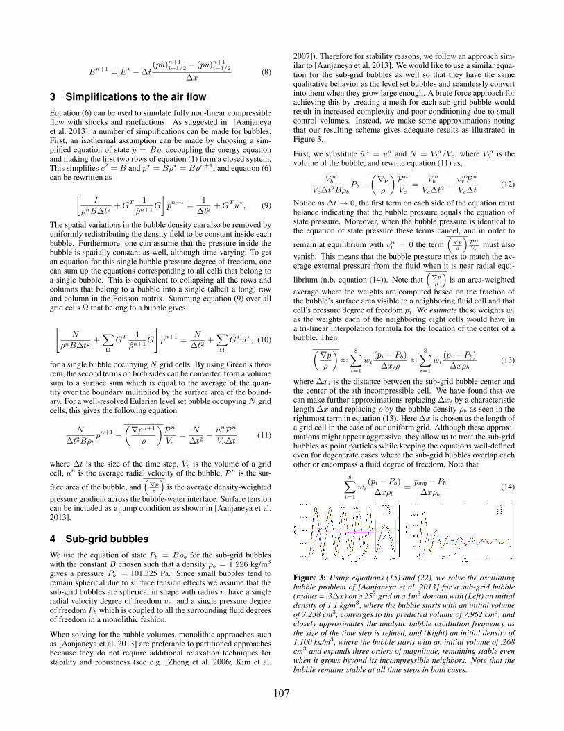
Figure 3: Using equations (15) and (22), we solve the oscillatingbubble problem of [Aanjaneya et al. 2013] for a sub-grid bubble(radius = .3∆x) on a 253 grid in a 1m3 domain with (Left) an initialdensity of 1.1 kg/m3, where the bubble starts with an initial volumeof 7.238 cm3, converges to the predicted volume of 7.962 cm3, andclosely approximates the analytic bubble oscillation frequency asthe size of the time step is refined, and (Right) an initial density of1,100 kg/m3, where the bubble starts with an initial volume of .268cm3 and expands three orders of magnitude, remaining stable evenwhen it grows beyond its incompressible neighbors. Note that thebubble remains stable at all time steps in both cases.

107

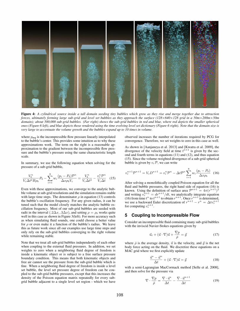
Figure 4: A cylindrical source inside a tall domain seeding tiny bubbles which grow as they rise and merge together due to attractionforces, ultimately forming large sub-grid and level set bubbles as they approach the surface (128×640×128 grid in a 50m×200m×50mdomain); about 500,000 sub-grid bubbles. (Far right) shows the sub-grid bubbles in red and blue, where red depicts the smaller sphericalones (Figure 6 left), and blue depicts those rendered using the time evolving level set dictionary (Figure 6 right). Note that the domain size isvery large to accentuate the volume growth and the bubbles expand up to 10 times in volume.

where pavg is the incompressible flow pressure linearly interpolatedto the bubble’s center. This provides some intuition as to why theseapproximations work. The term on the right is a reasonable ap-proximation to the gradient between the incompressible flow pres-sure and the bubble’s pressure using the same characteristic lengthscale.

In summary, we use the following equation when solving for thepressure of a sub-grid bubble,

V nb

Vc∆t2BρbPb −

8Xi=1

wi(pi − Pb)Pn

∆xρbVc=

V nb

Vc∆t2− vn

r Pn

Vc∆t(15)

Even with these approximations, we converge to the analytic bub-ble volume at sub-grid resolutions and the simulation remains stablewith large time steps. The denominator ρ in equation (13) controlsthe bubble’s oscillation frequency. For any given radius, it can betuned such that the model closely matches the analytic bubble os-cillation frequency. Most of our sub-grid bubbles are seeded withradii in the interval (.2∆x, .3∆x), and setting ρ = ρb works quitewell in this case as shown in Figure 3(left). For more accuracy suchas when simulating fluid sounds, one could choose a better valuefor ρ or even make it a function of the bubble’s radius. We leavethis as future work since all our examples use large time steps andonly rely on the sub-grid bubbles converging to the right volumewhile remaining stable.

Note that we treat all sub-grid bubbles independently of each otherwhen coupling to the external fluid pressures. In addition, we setweights to zero when a neighboring fluid degree of freedom isinside a kinematic object or is subject to a free surface pressureboundary condition. This means that both kinematic objects andfree air cannot see the pressure from the sub-grid bubble which isfine. When a neighboring fluid degree of freedom is inside a levelset bubble, the level set pressure degree of freedom can be cou-pled to the sub-grid bubble pressures, except that this increases thedensity of the Poisson equation matrix repeatedly for every sub-grid bubble adjacent to a single level set region - which we have

observed increases the number of iterations required by PCG forconvergence. Therefore, we set weights to zero in this case as well.

As shown in [Aanjaneya et al. 2013] and [Kwatra et al. 2009], thedivergence of the velocity field at time tn+1 is given by the sec-ond and fourth terms in equations (11) and (12), and thus equation(15). Since the volume-weighted divergence of a sub-grid sphericalbubble is given by vrP , we can write

vn+1r Pn+1 = VcD

n+1 = vnr Pn −∆tPn

8Xi=1

wi(pi − Pb)

∆xρb(16)

After solving a monolithically coupled Poisson equation for all thefluid and bubble pressures, the right hand side of equation (16) isknown. Using the definition of surface area Pn+1 = 4π(rn+1)2

and writing vn+1r = drn+1/dt, we analytically integrate equation

(16) from time tn to tn+1 to obtain rn+1. Once rn+1 is determined,we use a backward Euler discretization of rn+1 − rn = ∆tvn+1

r

for computing vn+1r .

5 Coupling to Incompressible FlowConsider an incompressible fluid containing many sub-grid bubbleswith the inviscid Navier-Stokes equations given by

~ut + (~u · ∇)~u +∇p

ρ= ~g (17)

where ρ is the average density, ~u is the velocity, and ~g is the netbody force acting on the fluid. We discretize these equations on aMAC grid where we first explicitly update

~u? − ~un

∆t+ (~u · ∇)~u = ~g (18)

with a semi-Lagrangian MacCormack method [Selle et al. 2008],and then solve for the pressure via

∇ · ∇p

ρ=∇ · ~u?

∆t− ∇ · ~un+1

∆t(19)

108

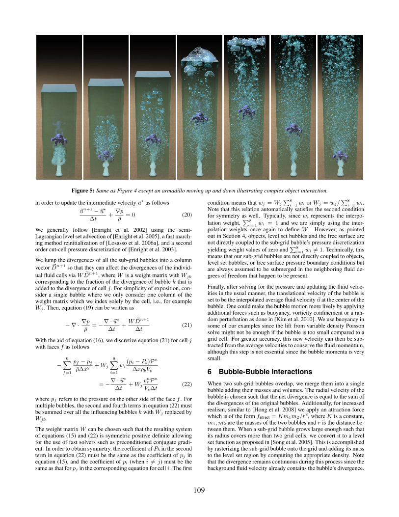
Figure 5: Same as Figure 4 except an armadillo moving up and down illustrating complex object interaction.

in order to update the intermediate velocity ~u? as follows~un+1 − ~u?

∆t+∇p

ρ= 0 (20)

We generally follow [Enright et al. 2002] using the semi-Lagrangian level set advection of [Enright et al. 2005], a fast march-ing method reinitialization of [Losasso et al. 2006a], and a secondorder cut-cell pressure discretization of [Enright et al. 2003].

We lump the divergences of all the sub-grid bubbles into a columnvector ~Dn+1 so that they can affect the divergences of the individ-ual fluid cells via W ~Dn+1, where W is a weight matrix with Wjk

corresponding to the fraction of the divergence of bubble k that isadded to the divergence of cell j. For simplicity of exposition, con-sider a single bubble where we only consider one column of theweight matrix which we index solely by the cell, i.e., for exampleWj . Then, equation (19) can be written as

−∇ · ∇p

ρ= −∇ · ~u?

∆t+

W ~Dn+1

∆t(21)

With the aid of equation (16), we discretize equation (21) for cell jwith faces f as follows

−6X

f=1

pf − pj

ρ∆x2+ Wj

8Xi=1

wi(pi − Pb)Pn

∆xρbVc

= −∇ · ~u?

∆t+ Wj

vnr Pn

Vc∆t(22)

where pf refers to the pressure on the other side of the face f . Formultiple bubbles, the second and fourth terms in equation (22) mustbe summed over all the influencing bubbles k with Wj replaced byWjk.

The weight matrix W can be chosen such that the resulting systemof equations (15) and (22) is symmetric positive definite allowingfor the use of fast solvers such as preconditioned conjugate gradi-ent. In order to obtain symmetry, the coefficient of Pb in the secondterm in equation (22) must be the same as the coefficient of pj inequation (15), and the coefficient of pi (when i 6= j) must be thesame as that for pj in the corresponding equation for cell i. The first

condition means that wj = Wj

P8i=1 wi or Wj = wj/

P8i=1 wi.

Note that this relation automatically satisfies the second conditionfor symmetry as well. Typically, since wi represents the interpo-lation weight,

P8i=1 wi = 1 and we are simply using the inter-

polation weights once again to define W . However, as pointedout in Section 4, objects, level set bubbles and the free surface arenot directly coupled to the sub-grid bubble’s pressure discretizationyielding weight values of zero and

P8i=1 wi 6= 1. Technically, this

means that our sub-grid bubbles are not directly coupled to objects,level set bubbles, or free surface pressure boundary conditions butare always assumed to be submerged in the neighboring fluid de-grees of freedom that happen to be present.

Finally, after solving for the pressure and updating the fluid veloc-ities in the usual manner, the translational velocity of the bubble isset to be the interpolated average fluid velocity ~u at the center of thebubble. One could make the bubble motion more lively by applyingadditional forces such as buoyancy, vorticity confinement or a ran-dom perturbation as done in [Kim et al. 2010]. We use buoyancy insome of our examples since the lift from variable density Poissonsolve might not be enough if the bubble is too small compared to agrid cell. For greater accuracy, this new velocity can then be sub-tracted from the average velocities to conserve the fluid momentum,although this step is not essential since the bubble momenta is verysmall.

6 Bubble-Bubble Interactions

When two sub-grid bubbles overlap, we merge them into a singlebubble adding their masses and volumes. The radial velocity of thebubble is chosen such that the net divergence is equal to the sum ofthe divergences of the original bubbles. Additionally, for increasedrealism, similar to [Hong et al. 2008] we apply an attraction forcewhich is of the form fattract = Km1m2/r2, where K is a constant,m1, m2 are the masses of the two bubbles and r is the distance be-tween them. When a sub-grid bubble grows large enough such thatits radius covers more than two grid cells, we convert it to a levelset function as proposed in [Song et al. 2005]. This is accomplishedby rasterizing the sub-grid bubble onto the grid and adding its massto the level set region by computing the appropriate density. Notethat the divergence remains continuous during this process since thebackground fluid velocity already contains the bubble’s divergence.

109

Also, when a sub-grid bubble enters a level set bubble we delete thesub-grid bubble and add its mass to the mass of the level set regionby modifying the density field.

If a level set bubble becomes smaller than a grid cell, it can losemass because of numerical errors during advection. However, thebubble mass cannot disappear because it is advected conservativelyusing the method of [Lentine et al. 2011]. This stray mass wasdistributed to the nearby bubbles in [Aanjaneya et al. 2013]. How-ever, such a scheme can sometimes move the bubble mass too faraway in a non-physical manner. Instead, we propose to track thisstray mass using sub-grid bubbles as shown in Figure 2. To achievethis, we first run a greedy condensation procedure on the stray den-sity field by moving it in the direction of the gradient vectors for afew iterations. Then for every cell with density above some thresh-old we seed a sub-grid bubble with the appropriate mass. To cor-rectly choose its volume, we set the steady state pressure p = ρIgh(where ρI is the density of the incompressible fluid and h is thedepth of the sub-grid bubble from the water surface) to be equal tothe equation of state pressure Pb = Bρb = BMb/Vb and solvefor Vb. Note that we do not use the incompressible pressure forcomputing the bubble’s volume because it can oscillate wildly andeven go negative at times during the course of the simulation dueto small numerical errors in the velocity field - this is because ofthe well-known fact that the fluid pressure in incompressible flowis more of a Lagrange multiplier (see [Majda 2001]) than an actualpressure. Finally note that even if our initial volume estimate hassome errors, the monolithic coupling keeps the scheme stable andthe bubble readily changes volume to an appropriate value.

In summary, starting from initial data containing level set and sub-grid bubbles and a volumetric field that represents the bubble mass,one loop of our pipeline runs as follows: the level set function isadvanced using the particle level set method of [Enright et al. 2002]and the bubble mass is advected using the unconditionally stable,fully conservative, semi-Lagrangian advection scheme of [Lentineet al. 2011]. After advection, the bubble mass and the level setfunction might be inconsistent as they are advanced using differentadvection schemes and also because some small level set bubblesmight have disappeared due to numerical errors during advection.To make them consistent, the mass surrounding a bubble is uni-formly redistributed such that the bubble density is spatially con-stant inside the bubble. Next, the sub-grid bubbles are advectedforward after applying forces such as buoyancy and attraction. Sub-sequently, inter-conversions are handled by merging overlappingbubbles, converting stray density to sub-grid bubbles and convert-ing large sub-grid bubbles to their corresponding level set represen-tation. Finally, a coupled system is solved where equation (11) iswritten per level set bubble, equation (15) per sub-grid bubble andthe standard incompressible flow equations with the modificationfor sub-grid bubbles, i.e., equation (22) in the rest of the fluid toget a pressure at every grid cell center as well as at every sub-gridbubble. This pressure is then used to update the fluid velocities andthe radial velocities of the sub-grid bubbles. To update the air ve-locities, we perform a second projection step using fluid velocitiesat the bubble-water interface as Neumann boundary conditions, asdescribed in [Aanjaneya et al. 2013].

7 Time-evolving proxy geometry

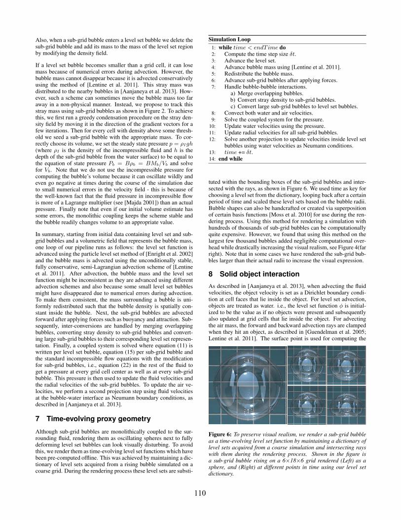
Although sub-grid bubbles are monolithically coupled to the sur-rounding fluid, rendering them as oscillating spheres next to fullydeforming level set bubbles can look visually disturbing. To avoidthis, we render them as time-evolving level set functions which havebeen pre-computed offline. This was achieved by maintaining a dic-tionary of level sets acquired from a rising bubble simulated on acoarse grid. During the rendering process these level sets are substi-

Simulation Loop1: while time < endT ime do2: Compute the time step size δt.3: Advance the level set.4: Advance bubble mass using [Lentine et al. 2011].5: Redistribute the bubble mass.6: Advance sub-grid bubbles after applying forces.7: Handle bubble-bubble interactions.

a) Merge overlapping bubbles.b) Convert stray density to sub-grid bubbles.c) Convert large sub-grid bubbles to level set bubbles.

8: Convect both water and air velocities.9: Solve the coupled system for the pressure.

10: Update water velocities using the pressure.11: Update radial velocities for all sub-grid bubbles.12: Solve another projection to update velocities inside level set

bubbles using water velocities as Neumann conditions.13: time += δt.14: end while

tuted within the bounding boxes of the sub-grid bubbles and inter-sected with the rays, as shown in Figure 6. We used time as key forchoosing a level set from the dictionary, looping back after a certainperiod of time and scaled these level sets based on the bubble radii.Bubble shapes can also be handcrafted or created via superpositionof certain basis functions [Moss et al. 2010] for use during the ren-dering process. Using this method for rendering a simulation withhundreds of thousands of sub-grid bubbles can be computationallyquite expensive. However, we found that using this method on thelargest few thousand bubbles added negligible computational over-head while drastically increasing the visual realism, see Figure 4(farright). Note that in some cases we have rendered the sub-grid bub-bles larger than their actual radii to increase the visual expression.

8 Solid object interaction

As described in [Aanjaneya et al. 2013], when advecting the fluidvelocities, the object velocity is set as a Dirichlet boundary condi-tion at cell faces that lie inside the object. For level set advection,objects are treated as water. i.e., the level set function φ is initial-ized to be the value as if no objects were present and subsequentlyalso updated at grid cells that lie inside the object. For advectingthe air mass, the forward and backward advection rays are clampedwhen they hit an object, as described in [Guendelman et al. 2005;Lentine et al. 2011]. The surface point is used for computing the

Figure 6: To preserve visual realism, we render a sub-grid bubbleas a time-evolving level set function by maintaining a dictionary oflevel sets acquired from a coarse simulation and intersecting rayswith them during the rendering process. Shown in the figure isa sub-grid bubble rising on a 6×18×6 grid rendered (Left) as asphere, and (Right) at different points in time using our level setdictionary.

110

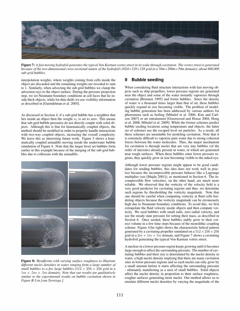
Figure 7: A fast moving hydrofoil generates the typical Von Karman vortex street in its wake through cavitation. The vortex street is generatedbecause of the two-dimensional cross-sectional nature of the hydrofoil (1024×128×128 grid in a 50m×200m×50m domain); about 600,000sub-grid bubbles.

interpolation weights, where weights coming from cells inside theobject are discarded and the remaining weights are rescaled to sumto 1. Similarly, when advecting the sub-grid bubbles we clamp theadvection rays to the object surface. During the pressure projectionstep, we set Neumann boundary conditions at cell faces that lie in-side thick objects, while for thin shells we use visibility informationas described in [Guendelman et al. 2005].

As discussed in Section 4, if a sub-grid bubble has a neighbor thatlies inside an object then the weight wi is set to zero. This meansthat sub-grid bubble pressures do not directly couple with solid ob-jects. Although this is fine for kinematically coupled objects, themethod should be modified in order to properly handle interactionswith two-way coupled objects, increasing the overall complexity.We leave this as interesting future work. Figure 5 shows a kine-matically coupled armadillo moving inside the underwater bubblesimulation of Figure 4. Note that the larger level set bubbles formearlier in this example because of the merging of the sub-grid bub-bles due to collisions with the armadillo.

Figure 8: Headforms with varying surface roughness to illustratedifferent nuclei densities in water ranging from a large number ofsmall bubbles to a few large bubbles (512 × 256 × 256 grid in a1m × .5m × .5m domain). Note that our results are qualitativelysimilar to the experimental results on bubble cavitation shown inFigure B.3 in [van Terwisga ].

9 Bubble seeding

When considering fluid structure interactions with fast moving ob-jects such as ship propellers, lower pressure regions are generatednear the object and some of the water instantly vaporizes throughcavitation [Brennen 1995] and forms bubbles. Since the densityof water is a thousand times larger than that of air, these bubblesquickly expand in size becoming visible. The problem of model-ing bubble generation has been addressed by various authors forphenomena such as boiling [Mihalef et al. 2006; Kim and Carl-son 2007] or air entrainment [Greenwood and House 2004; Honget al. 2008; Mihalef et al. 2009]. While the former schemes predictbubble seeding locations using temperature and objects, the latterset of schemes use the escaped level set particles. As a result, allthese schemes are unsuitable for modeling cavitation. Note that itis extremely difficult to vaporize pure water due to strong cohesionforces between the water molecules. Thus, the major mechanismfor cavitation is through nuclei that are very tiny bubbles (of theorder of microns) already present in water, or which are generatednear rough surfaces. When these bubbles enter lower pressure re-gions, they quickly grow in size becoming visible to the naked eye.

Although lower pressure regions might appear to be good candi-dates for seeding bubbles, this idea does not work well in prac-tice because the incompressible pressure behaves like a Lagrangemultiplier (see [Majda 2001]), as mentioned in Section 6. The in-compressible flow velocities, on the other hand, are much morereliable. We observed that the vorticity of the velocity field is avery good predictor for cavitating regions and thus, we determinesuch regions by thresholding the vorticity magnitude. Note thatone should be careful when computing vorticity at fluid cells bor-dering objects because the vorticity magnitude can be erroneouslyhigh due to Neumann boundary conditions. To avoid this, we firstextrapolate the fluid velocity inside objects and then compute vor-ticity. We seed bubbles with small radii, zero radial velocity, anduse the steady state pressure for setting their mass, as described inSection 6. Once seeded, these bubbles stably grow to their cor-rect volume in a few time steps because of the monolithic couplingscheme. Figure 1(far right) shows the characteristic helical patterngenerated by a cavitating propeller simulated on a 512×256×256grid in a 2m× 1m× 1m domain, and Figure 7 shows a cavitatinghydrofoil generating the typical Von Karman vortex street.

A nucleus in a lower pressure region keeps growing until it becomeslarge enough to affect the surrounding pressure. The number of cav-itating bubbles and their size is determined by the nuclei density inwater, a high nuclei density implying that there are many cavitationsites in lower pressure regions and so each nuclei can only grow bya small amount before it starts affecting the surrounding pressure- ultimately manifesting as a mist of small bubbles. Solid objectsaffect the nuclei density in proportion to their surface roughness,rougher surfaces generating more nuclei. Our method allows us toemulate different nuclei densities by varying the magnitude of the

111

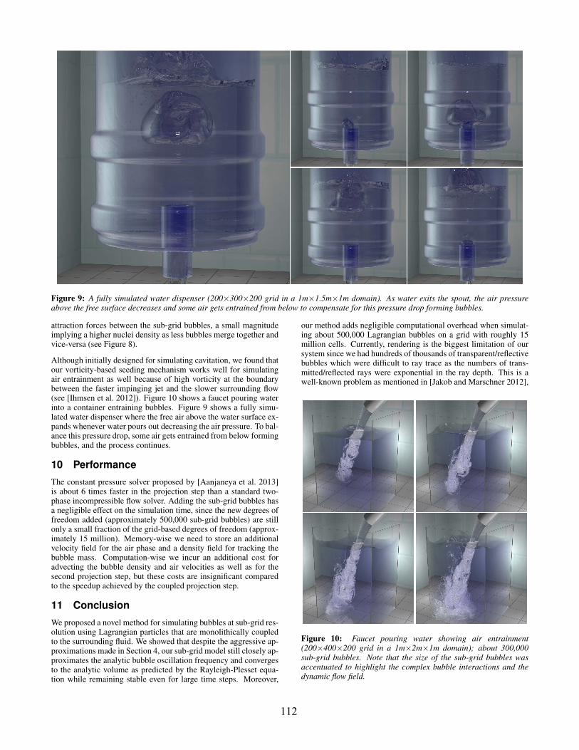
Figure 9: A fully simulated water dispenser (200×300×200 grid in a 1m×1.5m×1m domain). As water exits the spout, the air pressureabove the free surface decreases and some air gets entrained from below to compensate for this pressure drop forming bubbles.

attraction forces between the sub-grid bubbles, a small magnitudeimplying a higher nuclei density as less bubbles merge together andvice-versa (see Figure 8).

Although initially designed for simulating cavitation, we found thatour vorticity-based seeding mechanism works well for simulatingair entrainment as well because of high vorticity at the boundarybetween the faster impinging jet and the slower surrounding flow(see [Ihmsen et al. 2012]). Figure 10 shows a faucet pouring waterinto a container entraining bubbles. Figure 9 shows a fully simu-lated water dispenser where the free air above the water surface ex-pands whenever water pours out decreasing the air pressure. To bal-ance this pressure drop, some air gets entrained from below formingbubbles, and the process continues.

10 Performance

The constant pressure solver proposed by [Aanjaneya et al. 2013]is about 6 times faster in the projection step than a standard two-phase incompressible flow solver. Adding the sub-grid bubbles hasa negligible effect on the simulation time, since the new degrees offreedom added (approximately 500,000 sub-grid bubbles) are stillonly a small fraction of the grid-based degrees of freedom (approx-imately 15 million). Memory-wise we need to store an additionalvelocity field for the air phase and a density field for tracking thebubble mass. Computation-wise we incur an additional cost foradvecting the bubble density and air velocities as well as for thesecond projection step, but these costs are insignificant comparedto the speedup achieved by the coupled projection step.

11 Conclusion

We proposed a novel method for simulating bubbles at sub-grid res-olution using Lagrangian particles that are monolithically coupledto the surrounding fluid. We showed that despite the aggressive ap-proximations made in Section 4, our sub-grid model still closely ap-proximates the analytic bubble oscillation frequency and convergesto the analytic volume as predicted by the Rayleigh-Plesset equa-tion while remaining stable even for large time steps. Moreover,

our method adds negligible computational overhead when simulat-ing about 500,000 Lagrangian bubbles on a grid with roughly 15million cells. Currently, rendering is the biggest limitation of oursystem since we had hundreds of thousands of transparent/reflectivebubbles which were difficult to ray trace as the numbers of trans-mitted/reflected rays were exponential in the ray depth. This is awell-known problem as mentioned in [Jakob and Marschner 2012],

Figure 10: Faucet pouring water showing air entrainment(200×400×200 grid in a 1m×2m×1m domain); about 300,000sub-grid bubbles. Note that the size of the sub-grid bubbles wasaccentuated to highlight the complex bubble interactions and thedynamic flow field.

112

and we would like to explore better methods to render them faster.In addition, sub-grid bubbles are only coupled to the surroundingwater and not to each other, to level set bubbles or to objects, all ofwhich we would like to consider in future work.

12 Acknowledgements

Research was supported in part by ONR N00014-09-1-0101, ONRN-00014-11-1-0027, ONR N00014-11-1-0707, ARL AHPCRCW911NF-07-0027, and the Intel Science and Technology Centerfor Visual Computing. Computing resources were provided in partby ONR N00014-05-1-0479. We would like to thank Jure Leskovecand Christos Kozyrakis for additional computing resources as wellas Andrej Krevl and Jacob Leverich for helping us use those re-sources.

References

AANJANEYA, M., PATKAR, S., AND FEDKIW, R. 2013. A mono-lithic mass tracking formulation for bubbles in incompressibleflow. Journal of Computational Physics 247, 17–61.

BOYD, L., AND BRIDSON, R. 2012. Multiflip for energetic two-phase fluid simulation. ACM Trans. Graph. 31, 2, 16:1–16:12.

BRENNEN, C. E. 1995. Cavitation and Bubble Dynamics. OxfordUniversity Press, USA.

BUSARYEV, O., DEY, T. K., WANG, H., AND REN, Z. 2012.Animating bubble interactions in a liquid foam. ACM Trans.Graph. 31, 4, 63:1–63:8.

CLEARY, P. W., PYO, S. H., PRAKASH, M., AND KOO, B. K.2007. Bubbling and frothing liquids. ACM Trans. Graph. 26, 3.

ENRIGHT, D., MARSCHNER, S., AND FEDKIW, R. 2002. Ani-mation and rendering of complex water surfaces. ACM Trans.Graph. (SIGGRAPH Proc.) 21, 3, 736–744.

ENRIGHT, D., NGUYEN, D., GIBOU, F., AND FEDKIW, R. 2003.Using the particle level set method and a second order accu-rate pressure boundary condition for free surface flows. In Proc.4th ASME-JSME Joint Fluids Eng. Conf., number FEDSM2003–45144. ASME.

ENRIGHT, D., LOSASSO, F., AND FEDKIW, R. 2005. A fast andaccurate semi-Lagrangian particle level set method. Computersand Structures 83, 479–490.

FEDKIW, R., LIU, X.-D., AND OSHER, S. 2002. A generaltechnique for eliminating spurious oscillations in conservativeschemes for multiphase and multispecies euler equations. Int. J.Nonlinear Sci. and Numer. Sim. 3, 99–106.

FOSTER, N., AND FEDKIW, R. 2001. Practical animation of liq-uids. In Proc. of ACM SIGGRAPH 2001, 23–30.

GEIGER, W., LEO, M., RASMUSSEN, N., LOSASSO, F., ANDFEDKIW, R. 2006. So real it’ll make you wet. In SIGGRAPH2006 Sketches & Applications, ACM Press.

GREENWOOD, S. T., AND HOUSE, D. H. 2004. Better with bub-bles: enhancing the visual realism of simulated fluid. In Proc.of the 2004 ACM SIGGRAPH/Eurographics Symp. on Comput.Anim., 287–296.

GRETARSSON, J., AND FEDKIW, R. 2013. Fully conservative,robust treatment of thin shell fluid-structure interactions in com-pressible flows. Journal of Computational Physics 245, 160–204.

GUENDELMAN, E., SELLE, A., LOSASSO, F., AND FEDKIW, R.2005. Coupling water and smoke to thin deformable and rigidshells. ACM Trans. Graph. (SIGGRAPH Proc.) 24, 3, 973–981.

HONG, J.-M., AND KIM, C.-H. 2003. Animation of bubbles inliquid. Comput. Graph. Forum (Eurographics Proc.) 22, 3, 253–262.

HONG, J.-M., AND KIM, C.-H. 2005. Discontinuous fluids. ACMTrans. Graph. (SIGGRAPH Proc.) 24, 3, 915–920.

HONG, J.-M., LEE, H.-Y., YOON, J.-C., AND KIM, C.-H. 2008.Bubbles alive. ACM Trans. Graph. 27, 3, 48:1–48:4.

IHMSEN, M., AKINCI, N., AKINCI, G., AND TESCHNER, M.2012. Unified spray, foam and air bubbles for particle-basedfluids. Vis. Comput. 28, 6-8, 669–677.

JAKOB, W., AND MARSCHNER, S. 2012. Manifold exploration:a markov chain monte carlo technique for rendering scenes withdifficult specular transport. ACM Trans. Graph., 58:1–58:13.

KIM, T., AND CARLSON, M. 2007. A simple boiling module. InACM SIGGRAPH/Eurographics Symp. on Comput. Anim., 27–34.

KIM, B., LIU, Y., LLAMAS, I., JIAO, X., AND ROSSIGNAC, J.2007. Simulation of bubbles in foam with the volume controlmethod. ACM Trans. Graph. 26, 3.

KIM, D., SONG, O.-Y., AND KO, H.-S. 2010. A practical simula-tion of dispersed bubble flow. ACM Trans. Graph. 29, 70:1–70:5.

KIM, P.-R., LEE, H.-Y., KIM, J.-H., AND KIM, C.-H. 2012.Controlling shapes of air bubbles in a multi-phase fluid simula-tion. Vis. Comput. 28, 6-8, 597–602.

KWATRA, N., SU, J., GRETARSSON, J., AND FEDKIW, R. 2009.A method for avoiding the acoustic time step restriction in com-pressible flow. J. Comput. Phys. 228, 11, 4146–4161.

LEE, H.-Y., HONG, J.-M., AND KIM, C.-H. 2009. Interchange-able sph and level set method in multiphase fluids. Vis. Comput.25, 5-7, 713–718.

LENTINE, M., GRETARSSON, J., AND FEDKIW, R. 2011. An un-conditionally stable fully conservative semi-lagrangian method.J. Comput. Phys. 230, 2857–2879.

LOSASSO, F., FEDKIW, R., AND OSHER, S. 2006. Spatially adap-tive techniques for level set methods and incompressible flow.Computers and Fluids 35, 995–1010.

LOSASSO, F., SHINAR, T., SELLE, A., AND FEDKIW, R. 2006.Multiple interacting liquids. ACM Trans. Graph. (SIGGRAPHProc.) 25, 3, 812–819.

LOSASSO, F., TALTON, J., KWATRA, N., AND FEDKIW, R. 2008.Two-way coupled sph and particle level set fluid simulation.IEEE TVCG 14, 4, 797–804.

MAJDA, A. J. 2001. Vorticity and Incompressible Flow. Cam-bridge Univ Pr.

MIHALEF, V., UNLUSU, B., METAXAS, D., SUSSMAN, M., ANDHUSSAINI, M. 2006. Physics based boiling simulation. In SCA’06: Proc. of the 2006 ACM SIGGRAPH/Eurographics Symp. onComput. Anim., 317–324.

MIHALEF, V., METAXAS, D. N., AND SUSSMAN, M. 2009. Sim-ulation of two-phase flow with sub-scale droplet and bubble ef-fects. Comput. Graph. Forum.

113

MOSS, W., YEH, H., HONG, J.-M., LIN, M. C., ANDMANOCHA, D. 2010. Sounding liquids: Automatic sound syn-thesis from fluid simulation. ACM TOG 29, 3, 21:1–21:13.

MULLER, M., SOLENTHALER, B., KEISER, R., AND GROSS, M.2005. Particle-based fluid-fluid interaction. In Proc. of the 2005ACM SIGGRAPH/Eurographics Symp. on Comput. Anim., 237–244.

SELLE, A., FEDKIW, R., KIM, B., LIU, Y., AND ROSSIGNAC, J.2008. An Unconditionally Stable MacCormack Method. J. Sci.Comp. 35, 2, 350–371.

SONG, O.-Y., SHIN, H., AND KO, H.-S. 2005. Stable but nondis-sipative water. ACM Trans. Graph., 81–97.

THUREY, N., SADLO, F., SCHIRM, S., MULLER-FISCHER, M.,AND GROSS, M. 2007. Real-time simulations of bubbles andfoam within a shallow water framework. In SCA ’07: Proc. of2007 ACM SIGGRAPH/Eurographics symposium on Computeranimation, 191–198.

VAN TERWISGA, T. J. C. Cavitation on ship propellers. http://ocw.tudelft.nl/courses/marine-technology/cavitation-on-ship-propellers/.

ZHENG, C., AND JAMES, D. L. 2009. Harmonic fluids. ACMTrans. Graph. (SIGGRAPH Proc.) 28, 3, 37:1–37:12.

ZHENG, W., YONG, J.-H., AND PAUL, J.-C. 2006. Simula-tion of bubbles. In SCA ’06: Proceedings of the 2006 ACMSIGGRAPH/Eurographics symposium on Computer animation,325–333.

114