a hybrid inventory control policy for · pdf filea hybrid inventory control policy for medical...
TRANSCRIPT

A HYBRID INVENTORY CONTROL POLICY FOR
MEDICAL SUPPLIES IN HOSPITALS
A THESIS
SUBMITTED TO THE DEPARTMENT OF INDUSTRIAL
ENGINEERING
AND THE INSTITUTE OF ENGINEERING AND SCIENCE
OF BILKENT UNIVERSITY
IN PARTIAL FULFILLMENT OF THE REQUIREMENTS
FOR THE DEGREE OF
MASTER OF SCIENCE
By
Gökçe Akın
July, 2010

ii
I certify that I have read this thesis and that in my opinion it is full adequate, in scope
and in quality, as a dissertation for the degree of Master of Science.
___________________________________
Asst. Prof. Dr. Osman Alp (Advisor)
I certify that I have read this thesis and that in my opinion it is full adequate, in scope
and in quality, as a dissertation for the degree of Master of Science.
___________________________________
Asst. Prof. Dr. Murat Fadıloğlu
I certify that I have read this thesis and that in my opinion it is full adequate, in scope
and in quality, as a dissertation for the degree of Master of Science.
______________________________________
Asst. Prof. Dr. Banu Yüksel Özkaya
Approved for the Institute of Engineering and Sciences:
____________________________________
Prof. Dr. Levent Onural
Director of Institute of Engineering and Science

iii
ABSTRACT
A HYBRID INVENTORY CONTROL POLICY FOR MEDICAL
SUPPLIES IN HOSPITALS
Gökçe Akın
M.S. in Industrial Engineering
Advisor: Asst. Prof. Dr. Osman Alp
July, 2010
In this thesis, we consider the inventory control problem of medical supplies that
arises in a particular hospital environment. The items are stored in nursing stations
from where they are retrieved by the nurses and used for the needs of in-patients or
out-patients. The nursing stations are replenished from a central warehouse. Items are
moved between the hospital’s central warehouse and the nursing stations by a
capacitated porter cart. In the representative nursing station that we analyze, the need
for the medical supplies by the in-patients can arise at any time during day or night.
It is possible to replenish the nursing stations during the day time on a continuous
scale; however, this is not possible after-hours because the warehouse operates only
during regular working hours. For this particular setting, we propose a hybrid
inventory control policy which consists of a continuous review joint replenishment
policy to manage the day time demand and a periodic review policy to manage the
night time demand. The prior performance measure is set to satisfy the target service
levels in the nursing stations. For a special case of the problem with a single item, we
develop exact expressions to estimate the policy parameters. For the multi-item case,
we analyze the impact of the policy parameters on the service level targets by
simulating a representative system under different scenarios. Finally, we analyze a
sample data collected from a nursing station and prescribe methods to determine the
policy parameters.
Keywords: Medical supplies, inventory control, joint replenishment, service level,
health care system
iv
ÖZET
HASTANELERDEKİ TIBBİ SARF MALZEMELERİ İÇİN KARMA
ENVANTER KONTROL POLİTİKASI
Gökçe Akın
Endüstri Mühendisliği Yüksek Lisans
Tez Yöneticisi: Yrd. Doç. Dr. Osman Alp
Temmuz, 2010
Bu tezde, incelediğimiz bir hastane ortamında kullanılan tıbbi sarf malzemeleri için
bir envanter kontrol problemi incelenmiştir. Bu hastanede tıbbi sarf malzemeleri her
katta bulunan hasta bakım istasyonlarında belirli miktarlarda tutulmakta ve kat
hemşireleri tarafından yatan veya ayakta tedavi gören hastalar için kullanılmaktadır.
Hasta bakım istasyonları kapasiteli bir el arabası kullanılarak ana depodan yeniden
doldurulmaktadır. Ele alınan örnek katta tıbbi sarf malzemeleri için gün içerisinde
veya gece herhangi bir saatte talep görülebilmektedir. Gün içerisinde hasta bakım
istasyonları herhangi bir zamanda sürekli olarak yeniden doldurulabilirken; çalışma
saatleri dışında ana depo kapalı olduğu için bu mümkün olmamaktadır. Böyle bir
sisteme uygun olarak karma bir envanter politikası önerilmiştir. Bu politikada gün
içerisindeki envanter kontrolü için sürekli yeniden gözden geçirilen toplu sipariş
politikası önerilirken; gece için bir dönemsel gözden geçirme politikası önerilmiştir.
Performans kriteri, hedeflenen hizmet düzeyinin sağlanması olarak belirlenmiştir.
Özel bir durum olarak tek ürünlü sistemde politika parametrelerin elde edilebilmesi
için kesin ifadeler türetilmiştir. Çok ürünlü sistem için ise politika parametrelerinin
hizmet düzeyi üzerindeki etkileri gözlemlemek için sistem farklı senaryolar altında
simüle edilmiş ve parametre kestirimi için yöntemler önerilmiştir. Son olarak,
hastaneden alınan örnek data incelenmiş ve önerilen kestirim yöntemleri uygulanıp
değerlendirilmiştir.
Anahtar sözcükler: Tıbbi sarf malzemeler, envanter kontrolü, toplu sipariş, hizmet
düzeyi, sağlık sistemi

v
Acknowledgement
First of all, I would like to express my sincere gratitude to my supervisor Asst. Prof.
Dr. Osman Alp for his invaluable guidance and support during my graduate study.
He has supervised me with everlasting interest and motivation throughout this study.
I would like to thank once more for his encouraging advices on the other academical
issues, especially for the last two years.
I am also grateful to Asst. Prof. Dr. Murat Fadıloğlu and Asst. Prof. Dr. Banu Yüksel
Özkaya for accepting to read and review this thesis and for their invaluable
suggestions.
I would like to thank to Ankara Güven Hospital for letting me to analyze the hospital
and providing me the representative data for this study.
I would like to express my sincere thanks to Prof. Dr. İhsan Sabuncuoğlu, Assoc.
Prof. Dr. Bahar Yetiş Kara and (once more) Asst. Prof. Dr. Osman Alp, since they
have always trusted in me and appreciated my work as their teaching assistant for
two years.
I am indebted to my fiance Korhan Aras for his incredible support and
encouragement for six years. I am also lucky to have Uğur Cakova as one of my best
friends who is ready to listen to me, encourages me with his advices and comes up
instant solutions all the time. Additionally, I am thankful to Pelin Damcı (and
Mehmet Can Kurt), Gülşah Hançerlioğulları, Hatice Çalık, Ece Demirci, Efe Burak
Bozkaya (and Füsun Şahin Bozkaya), Esra Koca, Burak Paç, Can Öz, Yiğit Saç,
Emre Uzun and all other friends that I failed to mention here, for their invaluable
support and friendship during my graduate study.
Most importantly, I would like to express my deepest gratitude to my family for their
endless love and support throughout my life.

vi
Contents
1. Introduction .......................................................................................................... 1
2. Literature Review................................................................................................. 6
2.1. OR in Health Care Literature ......................................................................... 6
2.2. Inventory Control of Medical Supplies .......................................................... 7
2.3. Joint Replenishment Policies with an Emphasis on Service Levels ............. 8
3. System Description and Data Analysis ............................................................. 12
3.1. System Description ...................................................................................... 12
3.2. Data Analysis ............................................................................................... 14
4. Model and Policies ............................................................................................. 25
4.1. Definition of the Inventory Problem ............................................................ 25
4.2. Solution Approaches .................................................................................... 27
4.2.1. Our Proposed Control Policy .............................................................. 28
4.2.2. A Special Case: Single-Item ............................................................... 30

vii
5. Policy Parameters Estimation .......................................................................... 41
5.1. An Estimation Method to Find Policy Parameters ...................................... 41
5.2. The Simulation Results for the Inventory System ...................................... 46
6. Conclusion .......................................................................................................... 58
Appendix A. The Detailed Information of the Items ........................................... 65
Appendix B. Daily Demand Distributions of Some Items ................................... 73

viii
List of Figures
1.1. Health care sector supply chain............................................................................. 2
3.1. Medical supplies inventory system in the hospital ............................................. 13
3.2. Histogram with Gamma fit for the interarrival times of item ID51 .................... 18
3.3. Histogram with Gamma fit for item ID51 total demand per night ..................... 19
3.4. Histogram with Gamma fit for the interarrival times of item ID52 .................... 19
3.5. Histogram with Gamma fit for item ID52 total demand per night ..................... 20
3.6. Histogram with Gamma fit for the interarrival times of item ID122 .................. 20
3.7. Histogram with Gamma fit for item ID122 total demand per night ................... 21
3.8. Histogram with Gamma fit for the interarrival times of item ID95 .................... 21
3.9. Histogram with Gamma fit for item ID95 total demand per night ..................... 22
3.10. Histogram with Gamma fit for the interarrival times of item ID75 .................. 23
3.11. Histogram with Gamma fit for the interarrival times of item ID112 ................ 23
4.1. Demand structure ................................................................................................ 27
ix
4.2a. First example of the behavior of inventory level over time .............................. 32
4.2b. Second example of the behavior of inventory level over time.......................... 32
4.3. Illustration of the demand arrivals within for ...................... 34
B.1. Daily demand distributions for the item ID42 .................................................... 74
B.2. Daily demand distributions for the item ID51 .................................................... 74
B.3. Daily demand distributions for the item ID41 .................................................... 75
B.4. Daily demand distributions for the item ID146 .................................................. 75
B.5. Daily demand distributions for the item ID52 .................................................... 76
B.6. Daily demand distributions for the item ID122 .................................................. 76
x
List of Tables
3.1. Correlation analysis for A items ......................................................................... 16
3.2. Correlation analysis for B items .......................................................................... 17
3.3. Distributions of compound parts for A items day-time demands ....................... 18
3.4. Distributions of compound parts for B items day-time demands ....................... 22
3.5. Distributions of night-time demands for B items ................................................ 24
4.1. Notation ............................................................................................................... 31
5.1. Results for the Scenario 1 ................................................................................... 53
5.2. Results for the Scenario 2 ................................................................................... 53
5.3. Results for the Scenarios 3-5............................................................................... 54
5.4. Results for the Scenario 6 ................................................................................... 54
5.5. Results for the Scenario 7 ................................................................................... 55
5.6. Results for the Scenario 8 ................................................................................... 55
5.7. Results for the Scenario 9 ................................................................................... 56

xi
5.8. Results for the Scenarios 10 and 11 where and ............................ 56
A.1. Six months data for 195 medical items .............................................................. 66
A.2. Descriptive statistics of some items ................................................................... 71

1
Chapter 1
Introduction
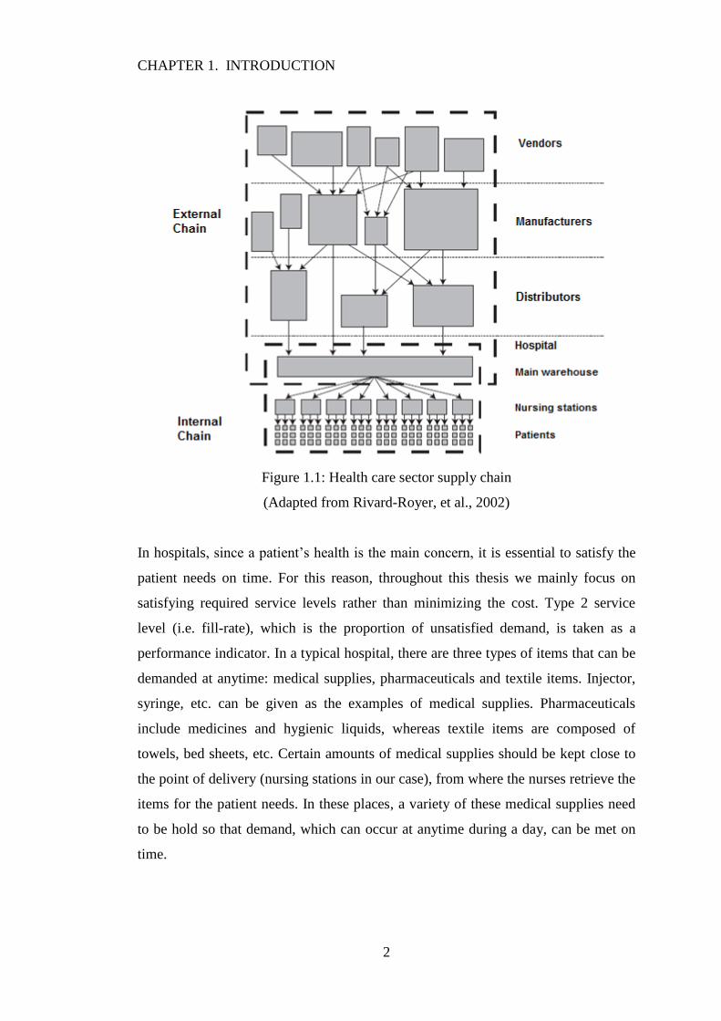
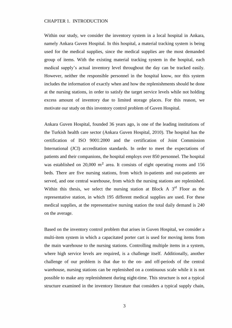
Health care sector supply chains are known to be structurally complicated and are
characterized by two chains: an external and an internal chain as shown in Figure 1.1
(Rivard-Royer, et al., 2002). Within this thesis, we do not consider the external
chain, instead we mainly focus on the internal chain which consists of the main
warehouse, the nursing stations and patients. In the internal chain, the nurses retrieve
the necessary items from the nursing stations for the patient needs and the nursing
stations are replenished by the main warehouse. Within hospitals, it is the top priority
to meet the patient needs on time, and hence inventory management plays a
significant role in hospital supply chains. As it is also underlined by Burns et al.
(2002), in the hospital supply chains the end users are not customers who are directly
paying for the item, but are the patients who create a demand at the nursing stations
due to clinical preference. For this reason, cost-benefit analysis or the budget
constraints are not considered as the main issue in the inventory management of
medical items.
CHAPTER 1. INTRODUCTION
2
Figure 1.1: Health care sector supply chain
(Adapted from Rivard-Royer, et al., 2002)
In hospitals, since a patient’s health is the main concern, it is essential to satisfy the
patient needs on time. For this reason, throughout this thesis we mainly focus on
satisfying required service levels rather than minimizing the cost. Type 2 service
level (i.e. fill-rate), which is the proportion of unsatisfied demand, is taken as a
performance indicator. In a typical hospital, there are three types of items that can be
demanded at anytime: medical supplies, pharmaceuticals and textile items. Injector,
syringe, etc. can be given as the examples of medical supplies. Pharmaceuticals
include medicines and hygienic liquids, whereas textile items are composed of
towels, bed sheets, etc. Certain amounts of medical supplies should be kept close to
the point of delivery (nursing stations in our case), from where the nurses retrieve the
items for the patient needs. In these places, a variety of these medical supplies need
to be hold so that demand, which can occur at anytime during a day, can be met on
time.
CHAPTER 1. INTRODUCTION
3
Within our study, we consider the inventory system in a local hospital in Ankara,
namely Ankara Guven Hospital. In this hospital, a material tracking system is being
used for the medical supplies, since the medical supplies are the most demanded
group of items. With the existing material tracking system in the hospital, each
medical supply’s actual inventory level throughout the day can be tracked easily.
However, neither the responsible personnel in the hospital know, nor this system
includes the information of exactly when and how the replenishments should be done
at the nursing stations, in order to satisfy the target service levels while not holding
excess amount of inventory due to limited storage places. For this reason, we
motivate our study on this inventory control problem of Guven Hospital.
Ankara Guven Hospital, founded 36 years ago, is one of the leading institutions of
the Turkish health care sector (Ankara Guven Hospital, 2010). The hospital has the
certification of ISO 9001:2000 and the certification of Joint Commission
International (JCI) accreditation standards. In order to meet the expectations of
patients and their companions, the hospital employs over 850 personnel. The hospital
was established on 20,000 area. It consists of eight operating rooms and 156
beds. There are five nursing stations, from which in-patients and out-patients are
served, and one central warehouse, from which the nursing stations are replenished.
Within this thesis, we select the nursing station at Block A 3rd
Floor as the
representative station, in which 195 different medical supplies are used. For these
medical supplies, at the representative nursing station the total daily demand is 240
on the average.
Based on the inventory control problem that arises in Guven Hospital, we consider a
multi-item system in which a capacitated porter cart is used for moving items from
the main warehouse to the nursing stations. Controlling multiple items in a system,
where high service levels are required, is a challenge itself. Additionally, another
challenge of our problem is that due to the on- and off-periods of the central
warehouse, nursing stations can be replenished on a continuous scale while it is not
possible to make any replenishment during night-time. This structure is not a typical
structure examined in the inventory literature that considers a typical supply chain,
CHAPTER 1. INTRODUCTION
4
such as a retail supply chain. We suggest a hybrid policy to be used for these two
distinct time frames. According to our proposed policy, the continuous review joint
replenishment policy is adapted during day-time, and periodic review
policy is used for the night-time in order to satisfy the target service levels, where
is set to one lead time ahead of the end of the day. The policy, is proposed by
Tanrikulu et al. (2009), and works in a way that, a fixed size of joint order is given
whenever an item’s inventory position drops below its reorder point ( ). In this
policy, the joint order size is allocated to other items so that all items’ inventory
positions in excess of their reorder points are equalized as far as they can be. This
policy leads to fully utilized porter cart (when is set to the cart capacity) at each
ordering instances, along with satisfying the target service levels by reviewing each
item’s inventory position continuously.
Before analyzing the inventory system under our proposed policy, we make a
detailed analysis of the transaction data collected from the representative nursing
station and classify the items in three classes A, B and C according to total demand
proportion of each item within the inventory system. Then, for a sample set of items,
we obtain the detailed statistics and probability distributions of item demands, in
order to use in our numerical analysis.
We derive exact expressions to find optimal policy parameters for the single item
case. However, since it is computationally hard to derive these expressions for the
multi item case, , we analyze the impact of the policy parameters on
the service level targets by simulating a representative system under different
scenarios. We simulate the inventory system by using Arena and starting our search
from the initial values that we estimate by considering the service levels, we obtain
the optimal parameter values. We find out that the method for estimating the initial
values gives the optimal values, while the method for estimating the initial values
gives overestimated values.
The remaining of this thesis is organized as follows. In Chapter 2, the related
literature is examined in three main parts, which are OR in health care, inventory
CHAPTER 1. INTRODUCTION
5
control of medical supplies, and joint replenishment policies with an emphasis on
service levels. Afterwards, we describe the system under consideration along with
the data analysis in detail in Chapter 3. In Chapter 4, after explaining the inventory
problem on hand, solution approaches are proposed for this problem. After
discussing the optimal policies, the proposed hybrid policy for our system is
introduced. Also in Chapter 4, the single-item case is analyzed and expressions are
derived for obtaining the optimal policy parameters for this special case. Policy
parameters estimation methods are introduced in Chapter 5, so that estimated values
close to the optimal values of the parameters can be obtained easily, without dealing
with complicated structures for the multi-item case. We test these methods by
simulating the system in Arena under different scenarios as they are explained in
Chapter 5. Finally, by Chapter 6 we conclude the thesis with our conclusion and
possible future extensions.
6
Chapter 2
Literature Review
2.1 OR in Health Care Literature
OR in Health Care literature is composed of three main areas: Health Care
Operations Management, Clinical Applications, and Health Care Policy and
Economic Analysis (Brandeau, et al., 2004). Health Care Operations Management
includes OR applications on managerial issues in hospitals such as designing
services, designing and managing the health care supply chain, facility planning and
designing, equipment evaluation and selection, process selection, capacity planning
and management, demand and capacity forecasting, scheduling and workforce
planning, resource allocation in medical environments, etc. Few examples in this
area are as follows: Green (2004) introduces the OR applications on hospital capacity
planning, Henderson et al. (2004) propose a decision making model for ambulance
service, and Daskin et al. (2004) explain how the facility location models can be
applied in health care. The second area, Clinical Applications, involves topics like
designing and planning of treatments for the patients, assessing how a disease is
likely to progress in a patient and choosing drugs, determining dosages and designing
other aspects, etc. In this area, studies are mostly focused on applying OR methods to

CHAPTER 2. LITERATURE REVIEW
7
the cancer detection and various type of therapies. Some examples in this area can be
given as follows: Maillart et al. (2008) study the breast cancer screening policies
dynamically, Lee et al. (2008) work on the planning of dialysis theraphy and Lee and
Zaider (2008) introduce a dynamic method for the treatment of prostate cancer. The
third area, which is Health Care Policy and Economic Analysis, includes topics such
as coordination of influenza vaccination, prediction of Health Care costs for a
government, drug policy etc. Some studies within this area can be given as, Chick et
al. (2008)’s work on supply chain coordination of the influenza vaccines and the
study of Bertsimas et al. (2008) on the prediction of health care costs. In this thesis,
we focus on the inventory control problem of medical supplies that arises in
hospitals. For this reason, our study falls into Health Care Operations Management
area.
2.2 Inventory Control of Medical Supplies
Even the inventory control literature has a wide range, the studies on specifically the
inventory control of medical supplies (e.g. syringe, mask, etc.) are limited. To begin
with, there are some studies on the general structure of hospital supply chains for the
medical supplies. Nicholson et al. (2004) analyze the cost and service level effect of
reducing the three echelon system, which involves item movements between
suppliers, main warehouse, nursing stations and patients, to a two echelon system in
which the main warehouse is removed. In their proposed system, an outside company
manages, holds and distributes the items to the nursing stations. They find out that by
outsourcing the inventory management a better system can be obtained in terms of
efficiency, high service levels and low level of inventory throughout the hospital.
There are other studies on structural changes in the hospital inventory systems, such
as implementing just-in-time or stockless systems (Rivard-Royer, et al., 2002). As
an example, a case study is conducted on this topic by Kumar et al. (2008) to the
health care industry of Singapore. In that study they propose a new structure for the
hospital supply chains in which just-in-time applications are used and the total cost in
the supply chain is reduced.

CHAPTER 2. LITERATURE REVIEW
8
DeScioli et al. (2005) conduct a research on inventory control in a hospital, in which
Automated Point of Use system is proposed to be used for tracking each item’s
inventory level automatically. In that research, they consider inventory carrying
costs, ordering costs, stockout costs and replenishment lead time while deciding on
the inventory control policy. Firstly, they propose a standard base stock policy with
periodic review. In order to achieve the required service level, they make sure that
the order up to level of each item is high enough to satisfy the total demand over the
review period and the lead time. Secondly, they propose an policy with
periodic review, where is the economic order quantity for each item. At a periodic
review instance, for an item whose inventory position is below their reorder level
( ), an order amount of is given. Note that in both of these policies, they consider
the items individually and they do not use the joint replenishment in terms of setting
a total ordering quantity at an ordering instance. In the hospital that we analyze, there
is also a tracking system to control each item’s inventory level. However, our study
differs from that research in way that we consider a continuous review joint
replenishment system with a capacitated cart, which is used for moving the items
between the warehouse and the nursing stations.
For another standard hospital setting, which also includes a main warehouse and
nursing stations, an inventory policy for the medical supplies by considering space
restrictions is proposed by Little et al. (2008). In that study, the proposed inventory
control policy is a standard base stock policy, whose parameters are found by taking
service levels, frequency of deliveries, space constraints and criticality constraints
into account. They assume that the replenishment lead time of a nursing station is
zero and demand of each item is normally distributed. They obtain results for
replenishing every day, every three days and every five days. They state two
objectives for the service levels: maximizing the minimum service level and
maximizing the average service level. With this in mind, they analyze their results
according to the percentage of items at each service level, the average service level
and total amount of space used. According to their analysis demand is a more
important guide to obtain high service levels rather than the unit volumes. They also
show that the same service levels can be reached by delivering everyday with a low

CHAPTER 2. LITERATURE REVIEW
9
space usage than delivering every three or five days with a high space usage. In our
research, we do not consider the space constraints explicitly; instead we try to
minimize the inventory level in the system while finding the joint replenishment
policy parameters. Moreover, in our study we consider each item’s service level
requirements separately and we make sure that each item is available with a required
service level by using a continuous review policy. Another difference of our study
from this research is that we also take the replenishment lead time into account.
2.3 Joint Replenishment Policies with an Emphasis on
Service Levels
In this section, we review the inventory control literature with an emphasis on joint
replenishment policies and service levels. Among the joint replenishment policies, in
policy, which is firstly proposed by Renberg et al. (1967), an order is placed to
raise each item’s inventory position to its own order-up-to level ( ), whenever the
total consumption reaches . Pantumsinchai (1992) compares this policy with
another joint ordering policy, the can order policy suggested by Balintfy
(1964). In that comparison paper, it is stated that policy is appropriate for the
inventory system in which the stockout costs are low and ordering costs are high.
Note also that depending on the problem parameters, has a strong advantage
when the high service levels are considered. This is because, by using the can order
policy, the inventory position of each item can be tracked and whenever an item’s
inventory position drops below its must order point ( ), a joint order is given for all
of the items, whose inventory positions are below their can order points ( ). Tracking
each item’s inventory positions is not possible for policy and once an item’s
inventory position drops below zero, if the total consumption is not at that time,
then that item may need to stay below zero for a long time, until the total
consumption reaches . Pantumsinchai (1992) also states that for most of the
problems with small lead times with large penalty costs policy ends up with
negative savings. Large penalty costs can be thought as high service levels, for this

CHAPTER 2. LITERATURE REVIEW
10
reason policy may not be appropriate for a system in which high service levels
are required. Moreover, Pantumsinchai (1992) compares policy with the
policies, which are proposed by Atkins et al. (1988), as well. According to
policy, each item’s inventory position is review every periods and a joint
order is given for increasing each item’s inventory position to its value.
Pantumsinchai (1992) states that the policy is comparable to policy.
Then, Viswanathan (1997) proposes another inventory control policy , which
involves policy with periodic ordering instances at every periods. In this
policy, every periods, inventory positions of all items are reviewed and a joint
order is given for the items, whose inventory positions are below their reorder points
( ) in order to raise them up to their order up to values ( ). Later on Nielsen et al.
(2005) suggest another policy in which the policy is used and inventory
positions are reviewed when the total consumption of all items reaches . They also
show that in all cases this policy is better than the periodic policy.
Moreover, for most of the cases it also outperforms policy (Nielsen, et al.,
2005).
Aside from these policies, Fung et al. (2001) proposes a periodic review policy
, which considers the coordinated replenishments for multi-item systems with
service level constraints as well as positive replenishment lead times. Note that in the
policy that is proposed by Atkins et al. (1988) the service level constraints are not
considered. For this reason policy of Fung et al. (2001) is better than
policy of Atkins et al. (1988) when the high service levels are required. Fung et al.
(2001) also compare the policy with policy and they find out that
there are significant savings of policy over for high service levels and
by using policy, positive lead time can easily be handled compared to
policy.
In a recent study, Ozkaya et al. (2006) suggest a joint replenishment policy, in which
a joint order is given to raise each item’s inventory position to its , when the total
consumption reaches to , or a total period of time passes (whichever is the first).
CHAPTER 2. LITERATURE REVIEW
11
They show that this policy is performing better than , , and
in most of the cases.
Lately, Tanrikulu et al. (2009) propose a new continuous review joint replenishment
policy . In this policy, a joint order size of is triggered whenever an item’s
inventory position drops below its reorder point ( ). is a fixed order amount, which
is set to the capacity of a truck or cart, depending on the environment in which the
policy is used. This fixed order size of , is allocated to all items in a way that each
item’s inventory position in excess of the reorder point are balanced. Since
capacitated equipment is used for the replenishment in the system under
consideration within this thesis, it is important to consider the capacity of that
equipment at each ordering instance. policy that is suggested by Cachon
(2001) also employs a fixed order size of at each replenishment and involves
continuous review. Comparison results of Tanrikulu et al. (2009) show that
policy outperforms the policy especially with the high backorder costs and
small lead time.
To sum up, this thesis contributes to both the inventory control literature and OR in
health care literature. By considering two distinct time frames, each requires high
service level; we suggest a hybrid policy, which consists of a continuous review
policy for the first time frame and a periodic review policy for the
second time frame, to be used. This part forms the main contribution of our thesis to
the inventory control literature. Moreover, since we find out that there is no study on
medical supplies inventory control which includes continuous review joint
replenishment policies, which utilize the capacitated cart at each ordering instance,
our study is also innovative for the OR in health care literature.
12
Chapter 3
System Description and Data Analysis
3.1 System Description
In a typical hospital, there are mainly three types of items to be controlled: medical
supplies, pharmaceuticals and textile items. Medical supplies consist of materials
such as injector, needle, cotton, bandage, etc. Pharmaceuticals are composed of
medicines and hygienic liquids like oxygen peroxide. For the textile items, towels,
bed sheets and patient cloths can be given as examples. In Guven Hospital, there are
three separate warehouses for these items. Medical supplies are stored in the central
warehouse, pharmaceuticals are stored in the pharmacy, and textile items are stored
in the textile warehouse. In this particular setting, we focus on the inventory control
of the medical supplies.
In Guven Hospital, medical supplies are controlled through a two echelon inventory
system. The upper echelon is the central warehouse and the lower echelon consists of
five nursing stations that are located at Block A 1st Floor, Block A 3
rd Floor, Block B
3rd
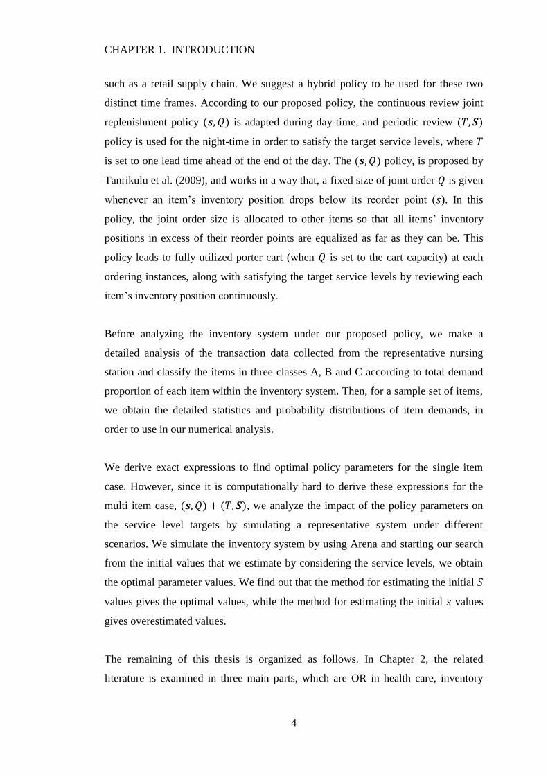
Floor, Emergency Room and Intense Care Unit. The corresponding inventory
system can be seen at Figure 3.1.

CHAPTER 3. SYSTEM DESCRIPTION AND DATA ANALYSIS
13
Figure 3.1: Medical Supplies Inventory System in the Hospital
In this system, inventories at the central warehouse are reviewed continuously by
using the inventory tracking system and orders for medical supplies are given to the
related suppliers whenever necessary. The procurement department of the hospital
makes contractual agreements with the suppliers. According to such contracts,
shipment related costs are covered by the suppliers and the suppliers agree to deliver
the items within a certain amount of time. After the arrival of the medical supplies,
the warehouse personnel enters the quantities of each item to the inventory tracking
system. In the central warehouse the medical supplies are stored until they are
requested and retrieved for the nursing stations. The central warehouse is operating
between 9:00 am and 6:00 pm. After 6:00 pm until 9:00 am next day, this warehouse
is closed and there cannot be any replenishment during this period.
The nursing stations serve directly to the patients. The patients to be served by the
stations can be either in-patient or out-patient. For example, Nursing Station-A3
serves in-patients while Nursing Station-ER serves mostly out-patients. All of the
nursing stations can observe demand throughout the day (24-hour period), regardless
of the time. Once a medical item is retrieved by a nurse for a patient need, the nurse
enters that record into the system by using the item’s barcode, so that they can track
Central
Warehouse
Suppliers
Patients
Nursing
Station-A1
Nursing
Station-B3
Nursing
Station-ER
Nursing
Station-ICU
Nursing
Station-A3
CHAPTER 3. SYSTEM DESCRIPTION AND DATA ANALYSIS
14
the remaining amount of inventory as well as the information of which item is used
for which patient. Nursing stations can be replenished by the central warehouse at
any time during central warehouse’s operating hours (9:00 am-6:00 pm), which we
call as the “day-time”, however, replenishment is not possible during its after hours
(6:00 pm-9:00 am next day), which we denote as the “night-time”. Whenever a
replenishment occurs at the nursing stations, each responsible nurse enters the
quantities of each item to the system and stores the items.
A porter cart is being used for the delivery of items from the central warehouse to the
nursing stations. The cart has a capacity in terms of volume. The same porter serves
more than one nursing station during day-time. After an order is given by a nursing
station, it takes about one hour to prepare and load the medical supplies on the cart,
and move these medical supplies to nursing stations. With this in mind, during the
last one hour just before the night-time begins, the nursing station does not place any
orders, since delivery is not possible in less than one hour and the nursing station
cannot be replenished before the end of the day.
Within this thesis, we focus on the inventory control operations at the nursing
stations and keep the operations at the central warehouse out of the scope. We take
the nursing station at Block A 3rd
Floor as the representative station, since it observes
demand for the highest variety of medical supplies compared to other stations.
Totally, there are 195 independent medical supplies used in this station. The analysis
of the types and demand rates of these supplies will be explained in the next section.
3.2 Data Analysis
As it is mentioned in the previous section, we choose the nursing station at Block A
3rd
Floor as the sample station. There are 195 different medical supplies that are used
in this station. We obtained detailed demand data of these medical items for six
months (April 1, 2009 - September 1, 2009). The demand data include the time of
each retrieval (by the nurses) instance of an item and the amount of items per
CHAPTER 3. SYSTEM DESCRIPTION AND DATA ANALYSIS
15
retrieval. Before analyzing this data, we prune them so that the outlier data, which
occur due to system failures, are removed.
First of all, we classify the items into three classes A, B and C according to total
demand proportion of each item within the inventory system. The related total
demand data are given in the Table A.1 in Appendix A. According to this
classification, A items constitute nearly 8% of the total number of items but
represents nearly 83% of the total demand in six months while B items make up 22%
of the total number of items but represents nearly 15% of the total demand. C items
constitute 70% of the total number of items but represents 2% of the total demand.
In Table A.1, A items average daily demand is within the range of 3 and 45. This is a
wide range because the first four items in this group have much higher demand than
the remaining items. The range of average daily demand for the B items is 0.17 and
3, and the rest of the items belong to the group C. Note that, the total daily demand of
all items is 240 on the average. We analyze the daily demands of some fast moving
items and obtain their descriptive statistics for the observed demand per day by using
Minitab. In Table A.2 in Appendix A, the related statistics are given for the first 42
items. Observe that the daily demands of A items have high level of variances, and
Gamma distribution turns out to be the best fitted distribution for these items’ daily
demands. Some A items’ histograms with distribution fits are given in Appendix B.
For the B items, none of the distributions can be fitted to the daily demands. Thus,
for this group of items we accumulate the daily demands into demands per 10 days
and then we fit Normal distribution to the total demand per 10 days. The C items
have very low daily demands, which may be observed once in a week or even once
in six months. Daily demand distribution fitting is not proper for these items. For this
reason, we analyze the time between demands and find out that the best distribution
which fits to the interarrival times of C items is the Exponential distribution. In other
words, during a day a C item’s demand is Poisson distributed. Since C items
constitute only 2% of all items and it is straightforward to set a policy under Poisson
demand, we exclude these items from further analysis.

CHAPTER 3. SYSTEM DESCRIPTION AND DATA ANALYSIS
16
Next, we analyze the daily demands to see if there is a correlation between items by
using Minitab. For this analysis we search for the dependency within the classes. In
Table 3.1 the correlation coefficients and p-values for the most demanded 10 items
from group A.
Table 3.1: Correlation analysis for A items (Correlation coefficient, p-values)
ID 41 51 42 52 122 146 20 95 44 74
41 - (0.201,
0.005)
(0.236,
0.001)
(0.209,
0.004)
(0.239,
0.001)
(0.044,
0.554)
(0.190,
0.009)
(0.113,
0.125)
(0.215,
0.003)
(0.125,
0.089)
51
- (0.15,
0.042)
(0.478,
0.000)
(0.46,
0.000)
(0.234,
0.001)
(0.500,
0.000)
(0.402,
0.000)
(0.032,
0.661)
(0.393,
0.000)
42
- (0.303,
0.000)
(0.169,
0.021)
(-0.033,
0.652)
(0.061,
0.411)
(0.128,
0.081)
(0.241,
0.001)
(0.003,
0.968)
52
- (0.396,
0.000)
(0.247,
0.001)
(0.396,
0.000)
(0.316,
0.000)
(0.102,
0.167)
(0.252,
0.001)
122
- (0.188,
0.010)
(0.358,
0.000)
(0.235,
0.001)
(0.039,
0.602)
(0.166,
0.024)
146
- (0.345,
0.000)
(0.355,
0.000)
(0.003,
0.963)
(0.247,
0.001)
20
- (0.464,
0.000)
(-0.017,
0.819)
(0.437,
0.000)
95
- (0.046,
0.530)
(0.587,
0.000)
44
- (0.033,
0.658)
74
-
According to this table, if p-values are smaller than 0.01, then there is sufficient
evidence that the correlations are not zero, otherwise the correlations between the
items are zero. With this in mind, there are 28 out of 45 pairs of items which are
correlated. Among these correlated pairs, the maximum absolute correlation
coefficient is 0.587 and the minimum absolute correlation coefficient is 0.188. In
Table 3.2 the correlation coefficients and p-values for a sample set of B items are
given. Among these items, only items ID75 and ID2 are correlated with each other
with a correlation coefficient of 0.211. For the C items we did not analyze the
correlations, since the demand rates for those items are so low and there is no
sufficient data for such analysis. Even we find out that there is a certain level of
CHAPTER 3. SYSTEM DESCRIPTION AND DATA ANALYSIS
17
correlation between some items, within this thesis we do not consider the
dependencies between the medical supplies.
Table 3.2: Correlation analysis for B items (Correlation coefficient, p-values)
ID 75 112 69 2 54
75 - (0.039,
0.592)
(0.003,
0.970)
(0.211,
0.003)
(0.081,
0.263)
112
- (-0.016,
0.828)
(0.139,
0.053)
(0.050,
0.490)
69
- (-0.010,
0.895)
(0.008,
0.917)
2
- (0.007,
0.926)
54
-
The system that we explain in the previous section makes it necessary for us to
obtain distinct demand structures for the day-time and night-time. Since a continuous
review policy is suitable for the day-time inventory control, we need to find the
distributions for the time between demands (i.e. interarrival times) and compounding
parts of these demands. On the other hand, since a periodic review policy is
appropriate for the night-time inventory control, the distribution for the demand per
night need to be obtained for each item. For this reason, we choose some
representative items from classes A and B, and analyze their demand structure in
detail by using Minitab. From Class A, we analyze the items ID51, ID52, ID122 and
ID95. From Class B, we analyze the items ID75 and ID112. Note that while deciding
the best fitted distribution for the related demand data, we use Minitab’s Anderson
Darling test and select the distribution with the sufficiently large p-value.
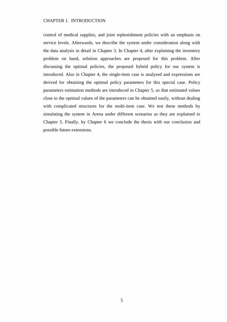
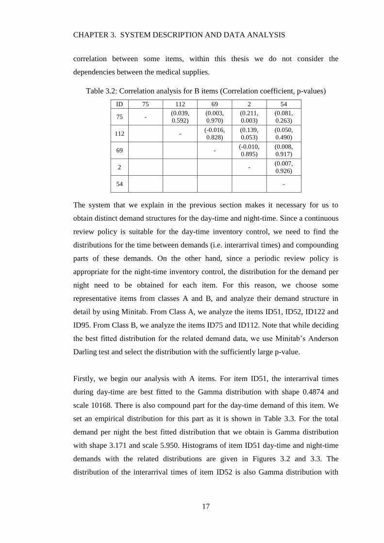
Firstly, we begin our analysis with A items. For item ID51, the interarrival times
during day-time are best fitted to the Gamma distribution with shape 0.4874 and
scale 10168. There is also compound part for the day-time demand of this item. We
set an empirical distribution for this part as it is shown in Table 3.3. For the total
demand per night the best fitted distribution that we obtain is Gamma distribution
with shape 3.171 and scale 5.950. Histograms of item ID51 day-time and night-time
demands with the related distributions are given in Figures 3.2 and 3.3. The
distribution of the interarrival times of item ID52 is also Gamma distribution with
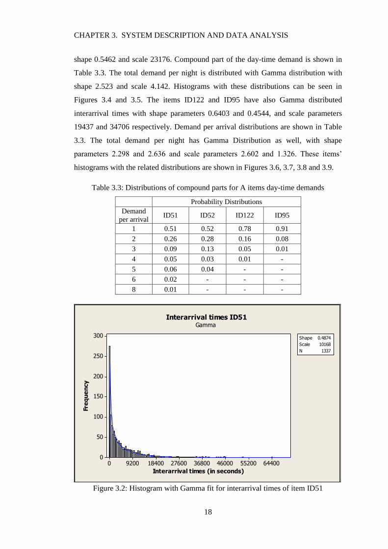
CHAPTER 3. SYSTEM DESCRIPTION AND DATA ANALYSIS
18
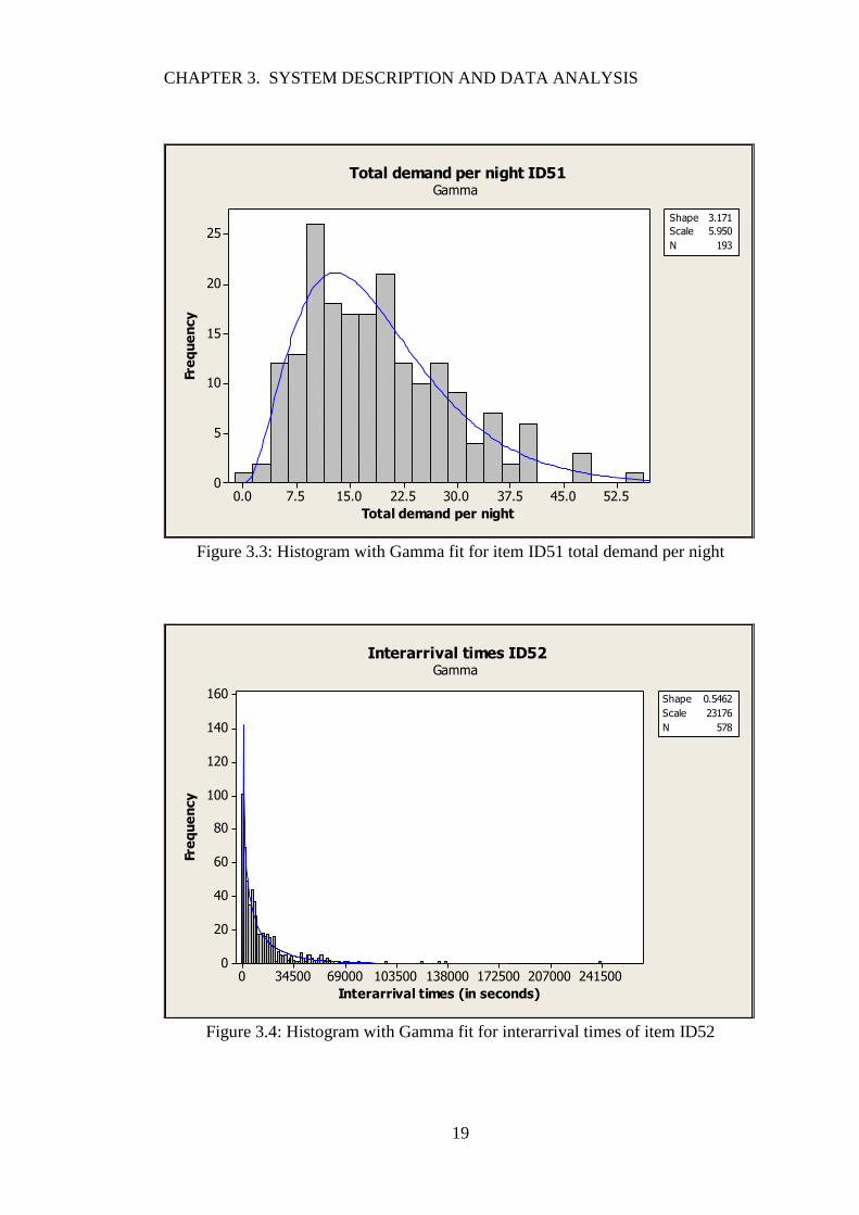
shape 0.5462 and scale 23176. Compound part of the day-time demand is shown in
Table 3.3. The total demand per night is distributed with Gamma distribution with
shape 2.523 and scale 4.142. Histograms with these distributions can be seen in
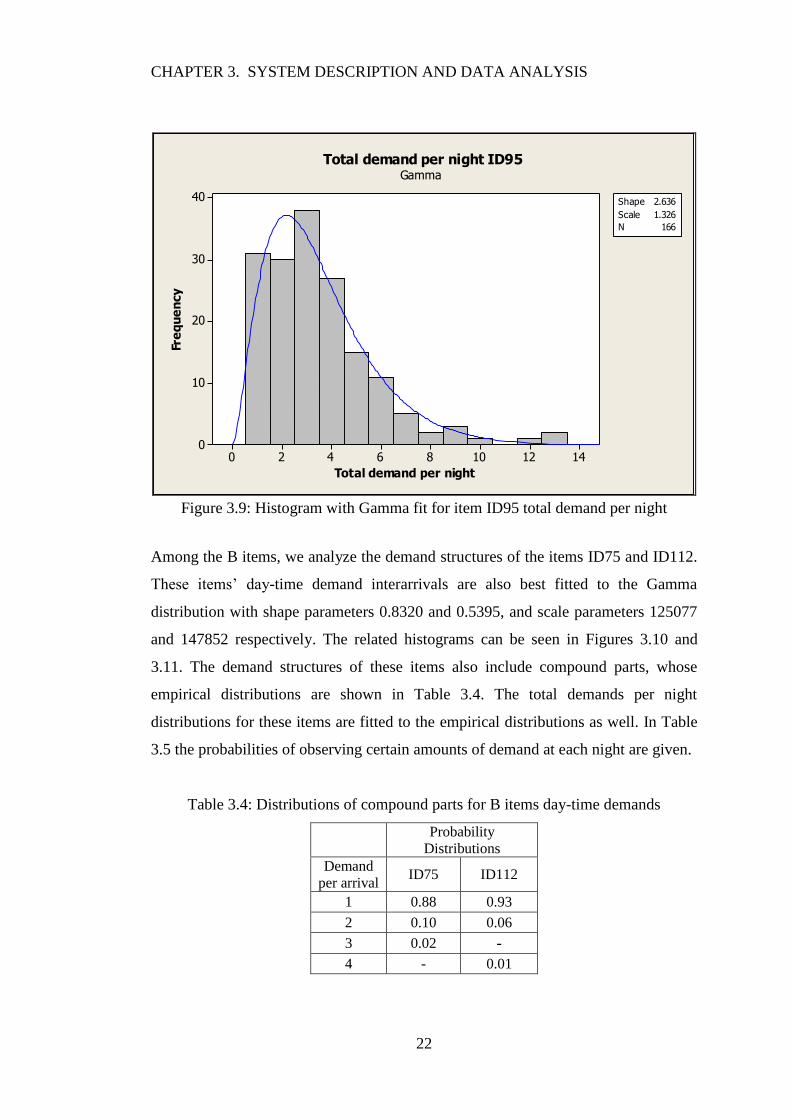
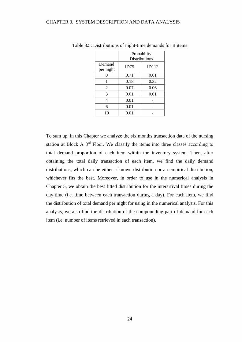
Figures 3.4 and 3.5. The items ID122 and ID95 have also Gamma distributed
interarrival times with shape parameters 0.6403 and 0.4544, and scale parameters
19437 and 34706 respectively. Demand per arrival distributions are shown in Table
3.3. The total demand per night has Gamma Distribution as well, with shape
parameters 2.298 and 2.636 and scale parameters 2.602 and 1.326. These items’
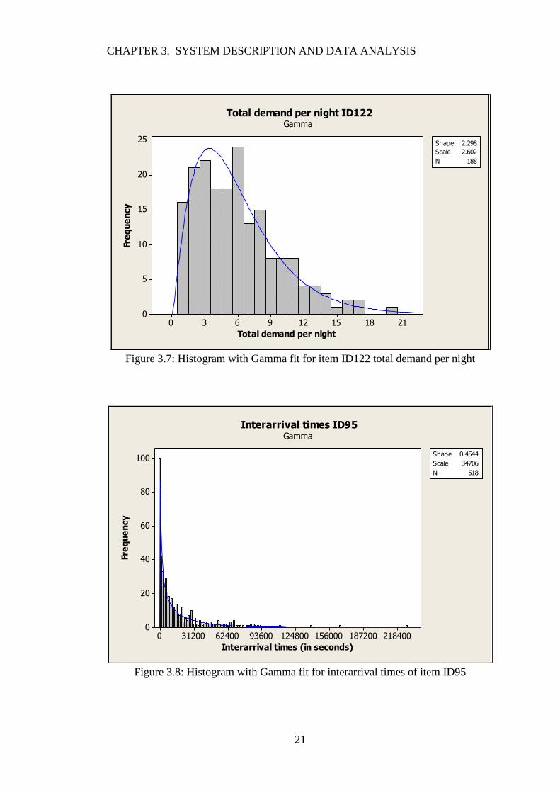
histograms with the related distributions are shown in Figures 3.6, 3.7, 3.8 and 3.9.
Table 3.3: Distributions of compound parts for A items day-time demands
Probability Distributions
Demand
per arrival ID51 ID52 ID122 ID95
1 0.51 0.52 0.78 0.91
2 0.26 0.28 0.16 0.08
3 0.09 0.13 0.05 0.01
4 0.05 0.03 0.01 -
5 0.06 0.04 - -
6 0.02 - - -
8 0.01 - - -
64400552004600036800276001840092000
300
250
200
150
100
50
0
Interarrival times (in seconds)
Fre
qu
en
cy
Shape 0.4874
Scale 10168
N 1337
Gamma
Interarrival times ID51
Figure 3.2: Histogram with Gamma fit for interarrival times of item ID51
CHAPTER 3. SYSTEM DESCRIPTION AND DATA ANALYSIS
19
52.545.037.530.022.515.07.50.0
25
20
15
10
5
0
Total demand per night
Fre
qu
en
cy
Shape 3.171
Scale 5.950
N 193
Gamma
Total demand per night ID51
Figure 3.3: Histogram with Gamma fit for item ID51 total demand per night
24150020700017250013800010350069000345000
160
140
120
100
80
60
40
20
0
Interarrival times (in seconds)
Fre
qu
en
cy
Shape 0.5462
Scale 23176
N 578
Gamma
Interarrival times ID52
Figure 3.4: Histogram with Gamma fit for interarrival times of item ID52
CHAPTER 3. SYSTEM DESCRIPTION AND DATA ANALYSIS
20
42363024181260
40
30
20
10
0
Total demand per night
Fre
qu
en
cy
Shape 2.523
Scale 4.142
N 181
Gamma
Total demand per night ID52
Figure 3.5: Histogram with Gamma fit for item ID52 total demand per night
805006900057500460003450023000115000
60
50
40
30
20
10
0
Interarrival times (in seconds)
Fre
qu
en
cy
Shape 0.6403
Scale 19437
N 573
Gamma
Interarrival times ID122
Figure 3.6: Histogram with Gamma fit for interarrival times of item ID122
CHAPTER 3. SYSTEM DESCRIPTION AND DATA ANALYSIS
21
211815129630
25
20
15
10
5
0
Total demand per night
Fre
qu
en
cy
Shape 2.298
Scale 2.602
N 188
Gamma
Total demand per night ID122
Figure 3.7: Histogram with Gamma fit for item ID122 total demand per night
2184001872001560001248009360062400312000
100
80
60
40
20
0
Interarrival times (in seconds)
Fre
qu
en
cy
Shape 0.4544
Scale 34706
N 518
Gamma
Interarrival times ID95
Figure 3.8: Histogram with Gamma fit for interarrival times of item ID95
CHAPTER 3. SYSTEM DESCRIPTION AND DATA ANALYSIS
22
14121086420
40
30
20
10
0
Total demand per night
Fre
qu
en
cy
Shape 2.636
Scale 1.326
N 166
Gamma
Total demand per night ID95
Figure 3.9: Histogram with Gamma fit for item ID95 total demand per night
Among the B items, we analyze the demand structures of the items ID75 and ID112.
These items’ day-time demand interarrivals are also best fitted to the Gamma
distribution with shape parameters 0.8320 and 0.5395, and scale parameters 125077
and 147852 respectively. The related histograms can be seen in Figures 3.10 and
3.11. The demand structures of these items also include compound parts, whose
empirical distributions are shown in Table 3.4. The total demands per night
distributions for these items are fitted to the empirical distributions as well. In Table
3.5 the probabilities of observing certain amounts of demand at each night are given.
Table 3.4: Distributions of compound parts for B items day-time demands
Probability
Distributions Demand
per arrival ID75 ID112
1 0.88 0.93
2 0.10 0.06
3 0.02 -
4 - 0.01

CHAPTER 3. SYSTEM DESCRIPTION AND DATA ANALYSIS
23
560000480000400000320000240000160000800000
10
8
6
4
2
0
Interarrival times (in seconds)
Fre
qu
en
cy
Shape 0.8320
Scale 125077
N 91
Gamma
Interarrival times ID75
Figure 3.10: Histogram with Gamma fit for interarrival times of item ID75
504000432000360000288000216000144000720000
20
15
10
5
0
Interarrival times (in seconds)
Fre
qu
en
cy
Shape 0.5395
Scale 147852
N 89
Gamma
Interarrival times ID112
Figure 3.11: Histogram with Gamma fit for interarrival times of item ID112
CHAPTER 3. SYSTEM DESCRIPTION AND DATA ANALYSIS
24
Table 3.5: Distributions of night-time demands for B items
Probability
Distributions Demand
per night ID75 ID112
0 0.71 0.61
1 0.18 0.32
2 0.07 0.06
3 0.01 0.01
4 0.01 -
6 0.01 -
10 0.01 -
To sum up, in this Chapter we analyze the six months transaction data of the nursing
station at Block A 3rd
Floor. We classify the items into three classes according to
total demand proportion of each item within the inventory system. Then, after
obtaining the total daily transaction of each item, we find the daily demand
distributions, which can be either a known distribution or an empirical distribution,
whichever fits the best. Moreover, in order to use in the numerical analysis in
Chapter 5, we obtain the best fitted distribution for the interarrival times during the
day-time (i.e. time between each transaction during a day). For each item, we find
the distribution of total demand per night for using in the numerical analysis. For this
analysis, we also find the distribution of the compounding part of demand for each
item (i.e. number of items retrieved in each transaction).
25
Chapter 4
Model and Policies
4.1 Definition of the Inventory Problem
We consider a multi-item two echelon inventory system where the upper echelon is a
central warehouse and the lower echelon involves smaller depots which are nursing
stations. We assume an ample supply at the central warehouse which is capable of
meeting the demand of nursing stations whenever necessary. The central warehouse
operates during a certain period of time of any given day, and is closed during the
remaining times. Due to such on- and off-periods of the central warehouse, it is
possible to replenish the nursing stations during the day-time on a continuous scale
but it is not possible to make any replenishment during the night-time.
In our setting, satisfying target service levels (i.e. fill rates) is the prior performance
measure rather than the cost measure, while making inventory control decisions.
Note that this priority is the natural choice for hospital operations. Nevertheless, we
still aim to minimize average inventory levels, because of the capacity of the nursing
stations and the inevitable cost considerations. In other words, we want to make sure
CHAPTER 4. MODEL AND POLICIES
26
that the average proportion of demand that cannot be met during day-time and night-
time should be less than a specified level with minimum average inventory levels.
During the first time frame (day-time), demand can be observed at anytime and a
capacitated cart is used for moving the items from upper echelon (the central
warehouse) to the lower echelon (nursing stations) whenever a replenishment occurs.
We denote the replenishment lead time by which starts at the time that an order is
given until it is received by the nursing station.
During the second time frame (night-time), demand can still be observed at anytime
at the nursing stations. However, the upper echelon is closed during this time frame
and for this reason replenishment cannot take place. This particular situation makes it
necessary to treat the day-time and night-time demand separately. Since
replenishment is possible at anytime during the day-time and achieving high service
levels targets is the main concern, controlling inventory at a continuous basis during
the day-time would be the most logical choice. However, since replenishment is not
possible during the night-time, the inventory control for this time period can only be
made at a periodic basis. In particular, a one time decision is made for the whole
night every day. Consequently, the day-time and night-time demands should be
modeled and handled differently. We assume a compound renewal type demand, i.e.
the interarrival times of the demand instances and compounding demand per arrival
are both random variables, for the day-time. On the other hand, the whole night-time
demand, which is also a random variable, is denoted by a single probability mass
distribution.
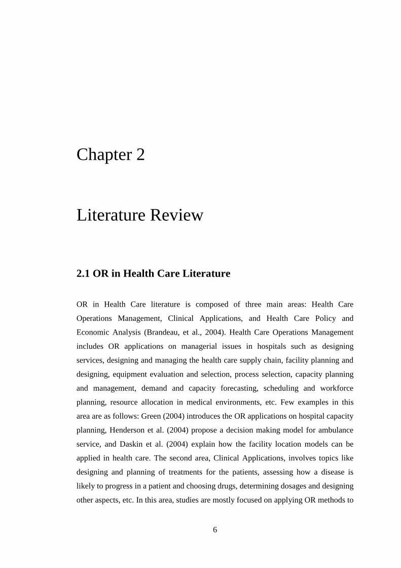
Consider a 24-hour period starting at some time . This starting time, , also marks
the start of the first time frame (day-time). The first time frame ends at time which
also marks the start of the second time frame (night-time). This second time frame
ends at time of the next 24-hour period. Let be the random variable denoting
the compounding part of the demand observed at a demand instance during day-time,
be the random variable denoting the interarrival times of the demand during day-

CHAPTER 4. MODEL AND POLICIES
27
time, and be the random variable denoting the accumulated total night-time
demand between and .
Figure 4.1: Demand structure
Within the scope of our problem, we assume that the medical supplies are
independent of each other. Note also that the total demand during night-time is
always greater than or equal to the total demand observed during lead time for each
medical supply in our particular context. Considering these assumptions and the
demand structure illustrated in Figure 4.1, we aim to find an appropriate inventory
control policy, which leads high service levels for both day-time and night-time
demand, while minimizing the average inventory levels.
4.2 Solution Approaches
Having two structurally different demand streams, as day-time and night-time
demands, yields a different inventory control problem than the typical ones. One
possible approach for this situation could be to obtain a non-stationary single demand
distribution by interlacing these two demand streams and search for the optimal
inventory control policies accordingly. By using this aggregated distribution, we may
find the optimal inventory control policies for this system; nevertheless, this
approach involves difficulties in terms of analyzing the system itself, since the
resulting distribution will have a time-dependent non-stationary structure. In this
thesis, we aim to find policies which are easy-to-implement and whose parameters
are easy to find for each medical supply.
Day 2 Day 1
a
n
d
e
n
d
a
t
a
n
d
e
n
d
a
t
a
n
d
e
n
d
a
t

CHAPTER 4. MODEL AND POLICIES
28
4.2.1 Our Proposed Control Policy
In our system, using a stationary inventory control policy with same parameters for
day-time and night-time is not an appropriate way to satisfy the high service levels
with low inventory levels. Because, this may cause high inventory levels during the
day-time in order to meet the night-time demand or on the contrary it may lead to
lower inventory levels but at the same time it may cause failure to satisfy the high
service levels during night-time. Thus, separate control policies or same policy with
different parameters for day-time and night-time demand can be used in order to
make sure that our operational targets are satisfied.
In order to take action before observing stockout at the medical supplies during day-
time, continuous review policies would be appropriate. Among the continuous
review policies, we search for the ones that are suitable for environments where high
service levels are required and a limit on the order size is imposed. For this reason,
policies which only consider high service levels but do not take limit on the order
size into account, such as and are eliminated (Tanrikulu et. al.,
2009). Since and policies take the capacity and utilization of that cart
into account, we take these policies as the candidate policies. The policy
employs a fixed order amount at each replenishment. Nevertheless, as it is
mentioned by Tanrikulu et. al. (2009), it does not take each item’s inventory levels
into consideration; instead under this policy replenishment is made when the total
demand of all items reaches . Therefore, this policy cannot respond quickly, if one
item’s inventory level drops below zero, before the total consumption reaches .
Another policy, which utilizes a constant order at each replenishment, is the
policy. This policy can also satisfy high service levels without carrying excess
amount of inventory. Tanrikulu et. al. (2009) points out that this policy outperforms
policy especially when the high service levels are required and lead times are
low. This comparison fits exactly our case when we think backorder costs as service
level requirements in our problem.

CHAPTER 4. MODEL AND POLICIES
29
Consequently, we propose policy to be used for day-time inventory control.
Under this policy, inventory positions of all items are reviewed continuously and
when one item’s inventory position drops to its reorder point , a fixed order is
given. In this joint order, each item’s order size is determined by a heuristic
allocation method, which is also used by Tanrikulu et.al. (2009), with the aim of
balancing each item’s inventory position in excess of the reorder point. Let be the
inventory position of item at any time and be the reorder level of item . By using
this allocation method, each item’s inventory position ( ) is brought above its
reorder level ( ). Moreover, since we use a capacitated cart for the replenishment
and we want it to be fully utilized, we allocate the remaining amount of in a way
that we balance each item’s inventory position in excess of its reorder level. We
allow for ordering more than one if it is necessary at an ordering instance. With
this in mind, our proposed allocation method is given below.
for
if
else
end
while
=
end
In order to satisfy the night-time demand, there is no need to hold inventory in
advance throughout the day-time, but giving an order, just one lead time before the
night-time starts would be sufficient. Thus, we suggest a periodic review policy for
night-time inventory control. In other words if the replenishment lead time is one

CHAPTER 4. MODEL AND POLICIES
30
hour, then controlling the inventory level and giving order if necessary at will
be appropriate for both satisfying night-time service levels and holding less
inventory. For the night-time inventory control, we propose policy, where
. By using this policy for the night-time demand, the necessary amount of
order, that is required to bring inventory positions up to each item’s , is given just a
lead time before the night-time demand is observed. Thus, without holding inventory
for a long time, high service levels can be satisfied for the night-time.
To sum up, we propose a hybrid policy, which involves continuous review
policy for the day-time demand and periodic review policy for the night-time
demand. Note that, in the multiple items case, of the policy and of the
policy are vectors of numbers corresponding to the reorder and order-up-to
points of items respectively. In the remainder, we do not include an index for items
for brevity but we note that each expression is valid for each item. In Chapter 5, we
will show how we can find the exact or estimated policy parameters for this hybrid
policy in order to satisfy the specified service levels.
4.2.2 A Special Case: Single-Item
In this section, we analyze a special case of our system: the single-item case. We
explain our approach for an item observing renewal type individual demand but this
approach can also be extended to compound demand situations. We develop exact
expressions that can be used to calculate different performance measures such as
total expected cost, service levels, etc. When there is only one item in the system,
then the proposed policy becomes the well known policy. In this special
case, we treat the night-time demand in the same way as it is in the multi-item case,
hence we suggest policy to be used for the night-time inventory control.
Summary of the notation used in the remainder is given in Table 4.1.

CHAPTER 4. MODEL AND POLICIES
31
Table 4.1: Notation
As explained in the previous section, at time , the inventory position of
the item is raised up to . Due to the nature of the system, no orders are placed
during and all outstanding orders at time would arrive until time
. Therefore, the inventory level at time before the night-time demand is
observed, , is given by
. Afterwards, the total demand for night-time
is observed which causes the inventory level at to drop to the value
and next day’s starting inventory position to take the value
which is equal to before any order is given in the next day as shown
at Figures 4.2a and 4.2b. We analyze two possible scenarios where the actions taken
at time are different. In Figure 4.2a observed night-time demand is so low that the
beginning inventory position is greater than the reorder point ( ) and
for this reason no order is given at the beginning of the next day.
: Reorder point for the day-time replenishment
: Fixed order amount for the day-time replenishment
: Periodic review instance for the night-time replenishment
: Order up to level for the night-time replenishment
: Replenishment lead time
: The start of the day-time
: The start of the night-time
: Random variable denoting the demand during lead time
: Random variable denoting the demand during night
: Amount of demand observed by time
: Inventory position at time
: Inventory level at time
: Inventory level at time after the order arrives for the night and before the
night’s demand is observed
i.e.
: Inventory level at time after the order arrives for the night and night’s
demand is observed
i.e.

CHAPTER 4. MODEL AND POLICIES
32
r
Figure 4.2a: First example for the behavior of inventory level over time
Figure 4.2b: Second example for the behavior of inventory level over time
Inventory Level
Time: t
:
:
Inventory Level
Time: t
:
:
r
r

CHAPTER 4. MODEL AND POLICIES
33
On the other hand, in Figure 4.2b total demand observed during night-time is high
enough that the inventory position at the beginning of the day ( ) drops below the
reorder point ( ) and an order is given at , in order to bring the inventory
position to or over . After the ordering is made at time , the inventory position
will take a value between and . After this, regular policy is
implemented until time at which the inventory position is raised to again for
the following night-time.
Rather than modeling this particular inventory system as a whole on an infinite
horizon continuous time scale, we model the inventory system for every “day-time”
(the time range from to ) separately, where the policy is employed on a
continuous time scale. Note that each “day-time” is stochastically equivalent to each
other. In this model, we also explicitly consider the effect of the policy. We
first develop exact expressions to estimate the probability distributions of the
inventory position at any given time where by using a transient
analysis, and then this information is used to find the probability distributions of the
inventory levels at any time .
When the system is controlled by the policy, takes a value between
and . A typical inventory system operated with the policy can be
modeled as continuous time Markov Chain by defining the states of the system as the
inventory position. Let for some time . Whenever a demand arrival
occurs after time , the system will move to the state if and to
the state if . Suppose that at a given time and for
some such that . Then the probability that is equal to at
another given time and for some such that , is the probability that there
are or or or ... demand arrivals during the time interval
. Similarly, the probability that is equal to for some ,
is the probability that there are or or ... demand arrivals during
the time interval .

CHAPTER 4. MODEL AND POLICIES
34
.
.
.
2 2 2 2 2
1 1
....... .......
2 2
2
3 3 3 3 3 3 3
3
The case for is illustrated in Figure 4.3. In this figure, the nodes represent
the inventory positions during the time interval . After starting at
, in order to end at the first possibility for the total demand
arrivals during , is , and is shown by the arcs, which are marked as “1”.
As the second possibility, the total demand may be equal to and this
situation can be obtained by starting with arcs “1” and continue with one full cycle
by using arcs “2”. The third possibility, which is , is shown by the arcs
“1”+“2”+“3”, in other words this possibility consists of arcs “1” followed by two full
cycles.
Figure 4.3: Illustration of the demand arrivals within for
The boundary conditions (initial conditions) for this model is given by the
probability distribution of the inventory position at time , i.e. .
The starting point of each day-time interval is and can be obtained as
follows. By conditioning on the smallest number of orders that can bring the
inventory position at the beginning of the day to or over the value ,
can be found.
if
then we do not give any order
.......
.
.
.
.
.
. .
.
.
.
.
.
.
.
.
.
.
. .
.
.

CHAPTER 4. MODEL AND POLICIES
35
if
if then we order Q
if
then order 2Q
if
then order 3Q
We can generalize this structure where
=
(4.1)
(4.2)
By substituting Equation (4.1) into (4.2), we obtain:
(4.3)
By using this information and the above discussion, we can calculate the inventory
position of the item at any given time as follows.
For the case when we drive the equations as follows:
. (4.4)

CHAPTER 4. MODEL AND POLICIES
36
Assume
...
Assume
...
We can generalize these expressions for where
and as:
. (4.5)
For the case when the structure of is different than the
previous case.
Assume
...
CHAPTER 4. MODEL AND POLICIES
37
Assume
...
We generalize these expressions for .
For and :
. (4.6)
For and :
. (4.7)
Actually, since for any distribution we can modify the interval for
in Equation (4.7) as .
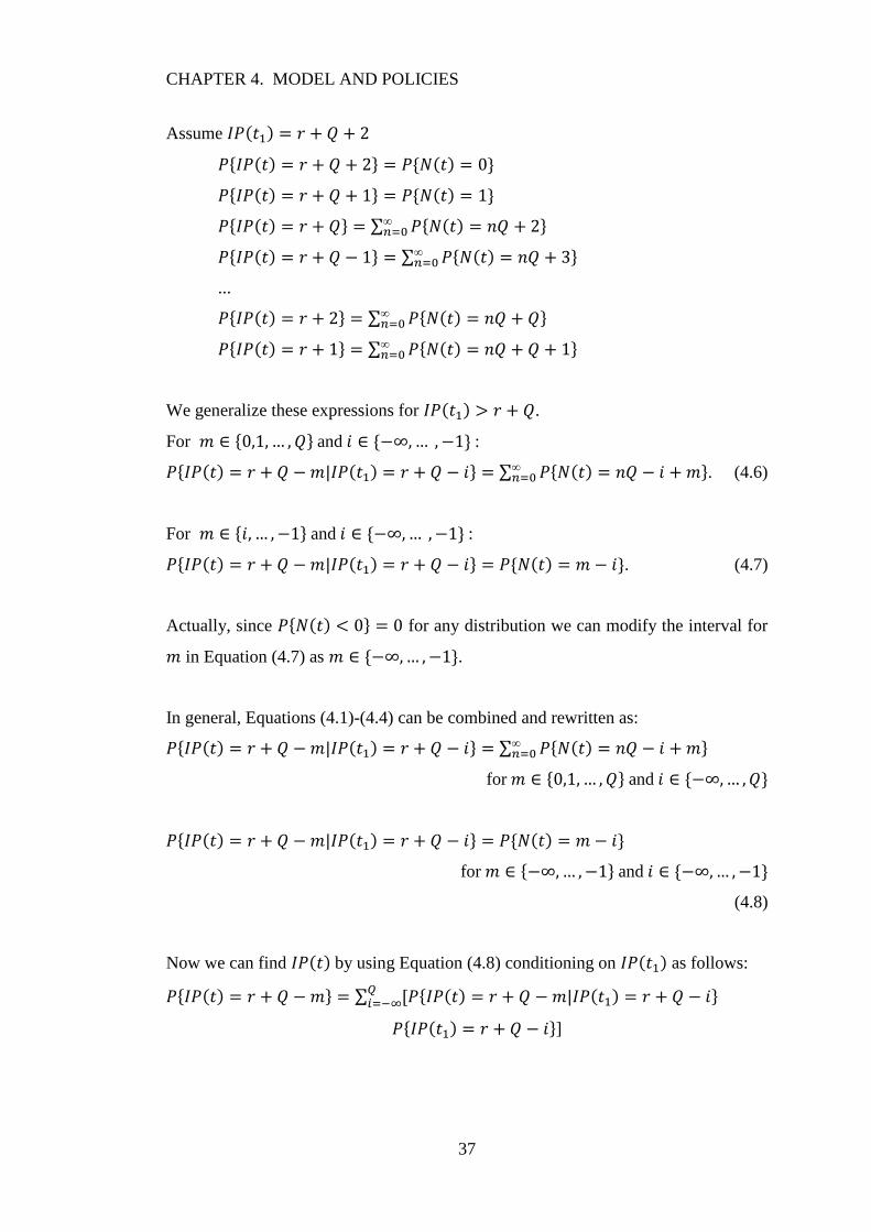
In general, Equations (4.1)-(4.4) can be combined and rewritten as:
for and
for and
(4.8)
Now we can find by using Equation (4.8) conditioning on as follows:
]
CHAPTER 4. MODEL AND POLICIES
38
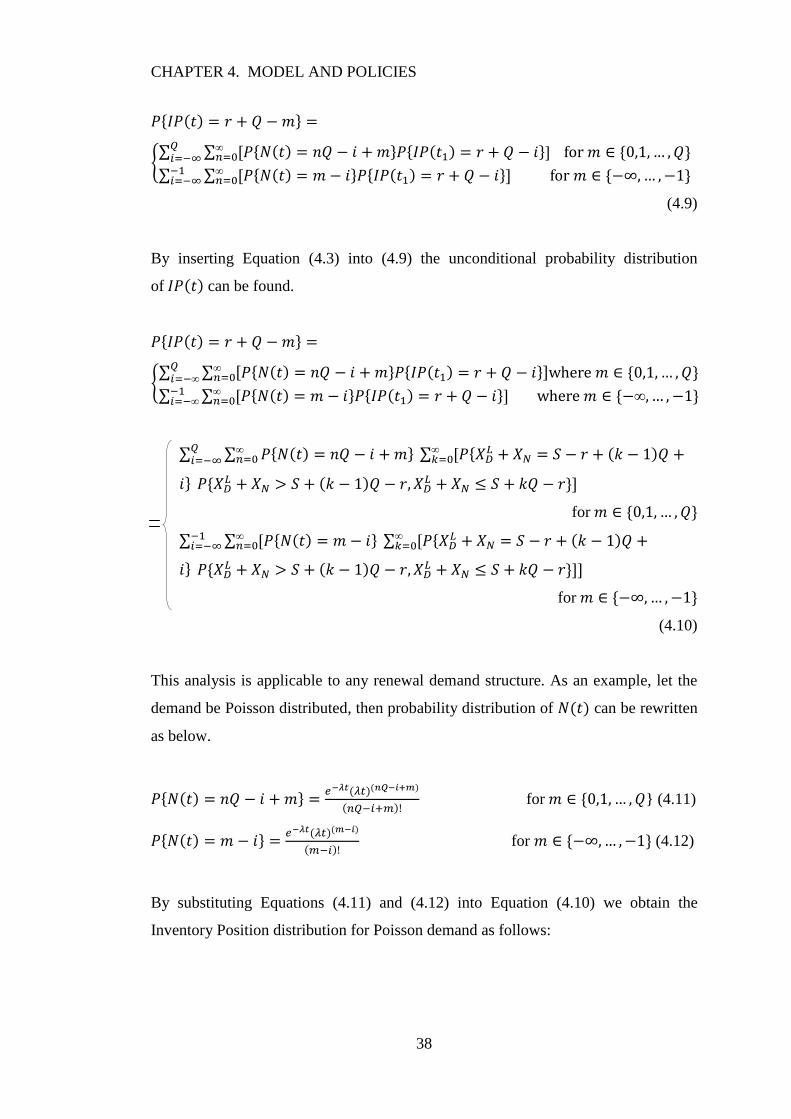
(4.9)
By inserting Equation (4.3) into (4.9) the unconditional probability distribution
of can be found.
for
for
(4.10)
This analysis is applicable to any renewal demand structure. As an example, let the
demand be Poisson distributed, then probability distribution of can be rewritten
as below.
for } (4.11)
for (4.12)
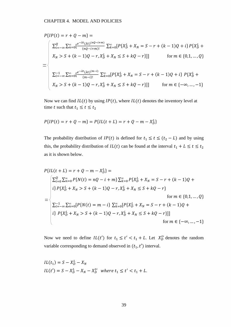
By substituting Equations (4.11) and (4.12) into Equation (4.10) we obtain the
Inventory Position distribution for Poisson demand as follows:
CHAPTER 4. MODEL AND POLICIES
39
for
for
Now we can find by using , where denotes the inventory level at
time such that
The probability distribution of is defined for and by using
this, the probability distribution of can be found at the interval
as it is shown below.
for
for
Now we need to define for . Let denotes the random
variable corresponding to demand observed in interval.
.
CHAPTER 4. MODEL AND POLICIES
40
By using these expressions exact analysis for the service levels can be made and the
optimal policy parameters for and can be found with specified service
level targets.
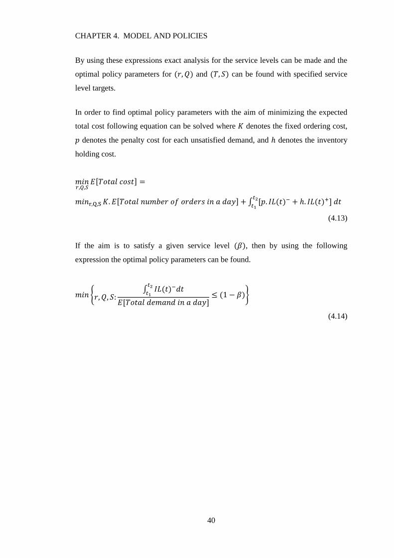
In order to find optimal policy parameters with the aim of minimizing the expected
total cost following equation can be solved where denotes the fixed ordering cost,
denotes the penalty cost for each unsatisfied demand, and denotes the inventory
holding cost.
(4.13)
If the aim is to satisfy a given service level , then by using the following
expression the optimal policy parameters can be found.
(4.14)

41
Chapter 5
Policy Parameters Estimation
In this Chapter, we aim to estimate the policy parameters in a way that the average
inventory level in the system is minimized. We propose methods to estimate the
policy parameters close to the optimal values. We test our methods by simulating the
inventory system in Arena under different scenarios in terms of demand distributions
and item variety, and analyze the impact of the policy parameters on the service
levels.
5.1 An Estimation Method to Find Policy Parameters
Recall from Chapter 4 that we propose the hybrid policy for the
inventory problem under concern. Our main aim is to make sure that the proportion
of unsatisfied demand is low enough to meet the required service levels. For this
reason, we suggest to use Type 2 service level expressions to find policy
parameters.

CHAPTER 5. POLICY PARAMETERS ESTIMATION
42
For the single-item case, we propose policy for the day-time demand and
policy for the night-time demand, as explained in Section 4.2.2. Either with
the purpose of obtaining the minimum cost or satisfying certain service levels, the
optimal policy parameters for these policies can be found by using the Equations
(4.13) and (4.14) respectively, which are obtained by using transient analysis for
inventory position as explained in Section 4.3.
For the multiple items case, estimating policy parameters is much more complicated.
Tanrikulu et al. (2009) develop a Markov Chain that can be used to model the
inventory positions realized under the policy. For items, this Markov Chain
has states. One might conduct a transient analysis for a multi item case similar to
the single item. However, such an approach would require extensive and complex
expressions to be solved. Therefore, finding policy parameters by using exact
analysis is not straightforward in our problem setting considering the high number of
items. By considering the computational difficulties of this analysis, we aim to
propose a practical and easy-to-use method to estimate policy parameters for the
multi-item case. We then validate our estimation method by comparing the estimated
parameters with the optimal parameters found by simulating the inventory control
system using Arena.
When the policies are implemented as explained, each of the policies
affect the inventory and service levels of the two distinct time frames. First of all,
Type 2 service level during the interval is dictated by the policy.
Recall that the inventory position of each item is raised to at time and
there cannot be any replenishment within time interval. Therefore, at the
beginning of the night-time (at time ), the inventory level, , is equal to
for each item, which is also equal to the inventory position at time . After
the night-time demand is observed, an order is placed either immediately at or at
some time later. In any case, the first order placed in day-time arrives at least a lead
time later than the beginning of the next day (i.e. at time or later). Thus, we
aim to find the value for each item in a way that we make sure that is high

CHAPTER 5. POLICY PARAMETERS ESTIMATION
43
enough to satisfy both the demand during night-time and the demand during first lead
time at the beginning of the next day with a certain probability. Type 2 service level
for this time frame can be estimated by:
With this in mind, the following expression can be used to estimate for each item
that will produce the required Type 2 service level:
(5.1)
During the remaining time of the day, i.e. in the interval, policy
affects the Type 2 service level. Recall in policy that a joint order is triggered,
when an item’s inventory position drops below its reorder level ( ). At that ordering
instance, along with this item, the other items’ inventory positions are increased
before reaching their values and the amount of increase depends on the allocation
policy employed and the current inventory positions of the items. In this system, it is
hard to track each item’s inventory position at an ordering instance and know whose
inventory position will drop below its reorder point and trigger the order, at the next
ordering instance. If we could estimate the inventory levels of all items at an ordering
instance, we could find the exact values that yield the required service levels.
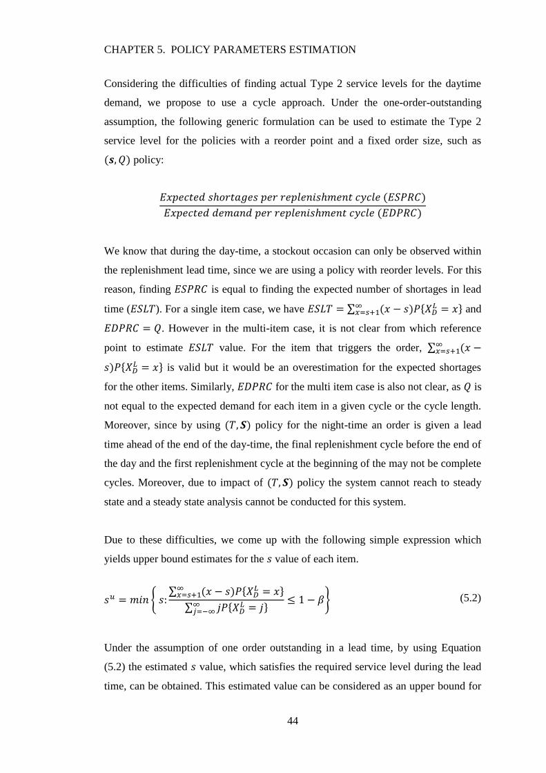
CHAPTER 5. POLICY PARAMETERS ESTIMATION
44
Considering the difficulties of finding actual Type 2 service levels for the daytime
demand, we propose to use a cycle approach. Under the one-order-outstanding
assumption, the following generic formulation can be used to estimate the Type 2
service level for the policies with a reorder point and a fixed order size, such as
policy:
We know that during the day-time, a stockout occasion can only be observed within
the replenishment lead time, since we are using a policy with reorder levels. For this
reason, finding is equal to finding the expected number of shortages in lead
time ( ). For a single item case, we have
and
. However in the multi-item case, it is not clear from which reference
point to estimate value. For the item that triggers the order,
is valid but it would be an overestimation for the expected shortages
for the other items. Similarly, for the multi item case is also not clear, as is
not equal to the expected demand for each item in a given cycle or the cycle length.
Moreover, since by using policy for the night-time an order is given a lead
time ahead of the end of the day-time, the final replenishment cycle before the end of
the day and the first replenishment cycle at the beginning of the may not be complete
cycles. Moreover, due to impact of policy the system cannot reach to steady
state and a steady state analysis cannot be conducted for this system.
Due to these difficulties, we come up with the following simple expression which
yields upper bound estimates for the value of each item.
Under the assumption of one order outstanding in a lead time, by using Equation
(5.2) the estimated value, which satisfies the required service level during the lead
time, can be obtained. This estimated value can be considered as an upper bound for
(5.2)
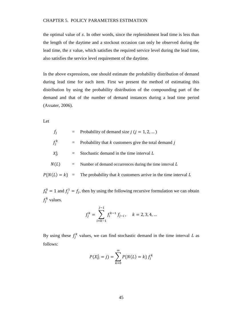
CHAPTER 5. POLICY PARAMETERS ESTIMATION
45
the optimal value of . In other words, since the replenishment lead time is less than
the length of the daytime and a stockout occasion can only be observed during the
lead time, the value, which satisfies the required service level during the lead time,
also satisfies the service level requirement of the daytime.
In the above expressions, one should estimate the probability distribution of demand
during lead time for each item. First we present the method of estimating this
distribution by using the probability distribution of the compounding part of the
demand and that of the number of demand instances during a lead time period
(Axsater, 2006).
Let
= Probability of demand size
= Probability that customers give the total demand
= Stochastic demand in the time interval
= Number of demand occurrences during the time interval
= The probability that customers arrive in the time interval
and
, then by using the following recursive formulation we can obtain
values.
By using these values, we can find stochastic demand in the time interval as
follows:

CHAPTER 5. POLICY PARAMETERS ESTIMATION
46
For items whose interarrival times are exponentially distributed, is
given by the Poisson distribution. For cases, with general interarrival distributions,
this probability can be estimated from the data by fitting a distribution to the number
of demand occurrences observed in each day. After finding the best fitted distribution
for the number of arrivals during lead time, we can insert that distribution as
in the formulation above and obtain stochastic demand in the time
interval .
To sum up, by using Equation (5.2) the overestimated value can be obtained for a
given day-time service level requirement and by using Equation (5.1) the exact value
of can be obtained for a given night-time service level requirement for each item.
Note that, this method is applicable to any renewal type of distribution.
In the next section, we find the optimal values through simulation in Arena and
gather insights on how to set the values in identical and non-identical multi item
situations, as well as insights on the proximity of the upper bounds to the optimal
values.
5.2 The Simulation Results for the Inventory System
We use Arena 11 for simulating the inventory system under the proposed
inventory control policies. We construct an allocation method in our
simulation so that the joint order is allocated to the items by balancing each item’s
inventory position in excess of its reorder point, as it is explained in Chapter 4. We
obtain and analyze the results for the identical and non-identical multi-item systems,
where we use Poisson and Gamma distributions for the day-time and night-time
demands. While analyzing the results, we focus on the effects of joint replenishment
(i.e. the interaction between the items), the effects of policy on policy,
and the effects of the fixed order size .

CHAPTER 5. POLICY PARAMETERS ESTIMATION
47
In order to find optimal policy parameters by simulating the system, we run the
simulation model for a sufficiently long time (92340 hours) by excluding a warm up
period (4860 hours), which we decide by using the Output Analyzer of Arena. For all
items, we use the exact values for parameters , which are found by using Equation
(5.1), and the upper bound values for parameters , which are obtained by using the
estimation expression given by Equation (5.2), as the initial values of our optimality
search and continue to search by decreasing the value until we find the optimal one.
First of all, we introduce the scenarios that we use for the analysis of the identical
multi-item case. Note that in all of the scenarios, we set the replenishment leadtime
(L) to 1 hour. As the first scenario, we take a system, which has identical four items
with Poisson distributed day-time and night-time demands. In the second scenario,
we test the system for identical four items with Poisson distributed demands with
lower demand rates. Then, we use another set of scenarios, in which different set of
identical items with Poisson distributed demands are used, in order to show the effect
of policy on the policy, if there is any. While constructing that set of
scenarios (Scenario 3, 4 and 5), we variate them in terms of the day-time and night-
time demand ratios. In the sixth and seventh scenarios we have identical four items
with Gamma distributed demands with high and low demanded items separately.
Scenario 1: Identical four-items with Poisson distribution (high demanded)
Item 1, 2, 3 and 4 lead time demand rate (
) : 2
Item 1, 2, 3 and 4 night-time demand rate ( ) : 18
Fixed order quantity ( ) : 24
Scenario 2: Identical four-items with Poisson distribution (low demanded)
Item 1, 2, 3 and 4 lead time demand rate (
) : 1
Item 1, 2, 3 and 4 night-time demand rate ( ) : 9
Fixed order quantity ( ) : 12
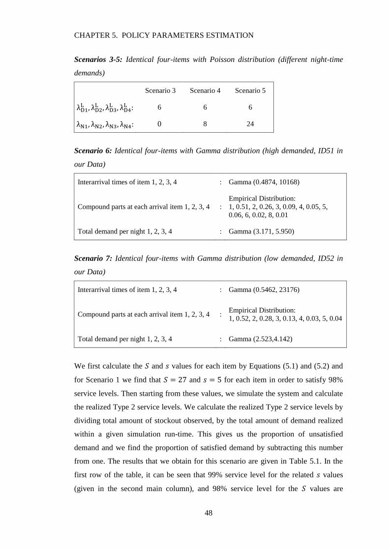
CHAPTER 5. POLICY PARAMETERS ESTIMATION
48
Scenarios 3-5: Identical four-items with Poisson distribution (different night-time
demands)
Scenario 3 Scenario 4 Scenario 5
6 6 6
0 8 24
Scenario 6: Identical four-items with Gamma distribution (high demanded, ID51 in
our Data)
Interarrival times of item 1, 2, 3, 4 : Gamma (0.4874, 10168)
Compound parts at each arrival item 1, 2, 3, 4 :
Empirical Distribution:
1, 0.51, 2, 0.26, 3, 0.09, 4, 0.05, 5,
0.06, 6, 0.02, 8, 0.01
Total demand per night 1, 2, 3, 4 : Gamma (3.171, 5.950)
Scenario 7: Identical four-items with Gamma distribution (low demanded, ID52 in
our Data)
Interarrival times of item 1, 2, 3, 4 : Gamma (0.5462, 23176)
Compound parts at each arrival item 1, 2, 3, 4 : Empirical Distribution:
1, 0.52, 2, 0.28, 3, 0.13, 4, 0.03, 5, 0.04
Total demand per night 1, 2, 3, 4 : Gamma (2.523,4.142)
We first calculate the and values for each item by Equations (5.1) and (5.2) and
for Scenario 1 we find that and for each item in order to satisfy 98%
service levels. Then starting from these values, we simulate the system and calculate
the realized Type 2 service levels. We calculate the realized Type 2 service levels by
dividing total amount of stockout observed, by the total amount of demand realized
within a given simulation run-time. This gives us the proportion of unsatisfied
demand and we find the proportion of satisfied demand by subtracting this number
from one. The results that we obtain for this scenario are given in Table 5.1. In the
first row of the table, it can be seen that 99% service level for the related values
(given in the second main column), and 98% service level for the values are
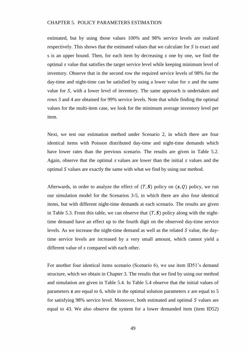
CHAPTER 5. POLICY PARAMETERS ESTIMATION
49
estimated, but by using those values 100% and 98% service levels are realized
respectively. This shows that the estimated values that we calculate for is exact and
s is an upper bound. Then, for each item by decreasing one by one, we find the
optimal value that satisfies the target service level while keeping minimum level of
inventory. Observe that in the second row the required service levels of 98% for the
day-time and night-time can be satisfied by using a lower value for and the same
value for , with a lower level of inventory. The same approach is undertaken and
rows 3 and 4 are obtained for 99% service levels. Note that while finding the optimal
values for the multi-item case, we look for the minimum average inventory level per
item.
Next, we test our estimation method under Scenario 2, in which there are four
identical items with Poisson distributed day-time and night-time demands which
have lower rates than the previous scenario. The results are given in Table 5.2.
Again, observe that the optimal values are lower than the initial values and the
optimal values are exactly the same with what we find by using our method.
Afterwards, in order to analyze the effect of policy on policy, we run
our simulation model for the Scenarios 3-5, in which there are also four identical
items, but with different night-time demands at each scenario. The results are given
in Table 5.3. From this table, we can observe that policy along with the night-
time demand have an effect up to the fourth digit on the observed day-time service
levels. As we increase the night-time demand as well as the related value, the day-
time service levels are increased by a very small amount, which cannot yield a
different value of compared with each other.
For another four identical items scenario (Scenario 6), we use item ID51’s demand
structure, which we obtain in Chapter 3. The results that we find by using our method
and simulation are given in Table 5.4. In Table 5.4 observe that the initial values of
parameters are equal to 6, while in the optimal solution parameters are equal to 5
for satisfying 98% service level. Moreover, both estimated and optimal values are
equal to 43. We also observe the system for a lower demanded item (item ID52)
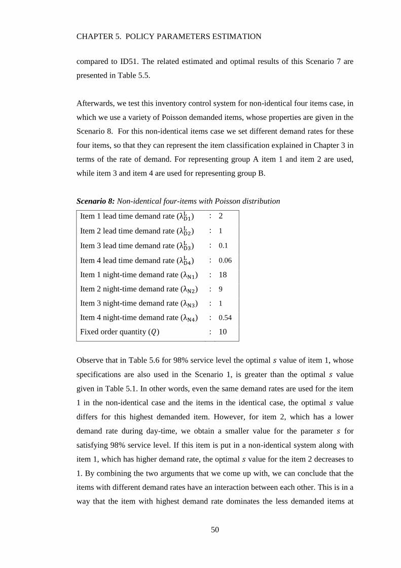
CHAPTER 5. POLICY PARAMETERS ESTIMATION
50
compared to ID51. The related estimated and optimal results of this Scenario 7 are
presented in Table 5.5.
Afterwards, we test this inventory control system for non-identical four items case, in
which we use a variety of Poisson demanded items, whose properties are given in the
Scenario 8. For this non-identical items case we set different demand rates for these
four items, so that they can represent the item classification explained in Chapter 3 in
terms of the rate of demand. For representing group A item 1 and item 2 are used,
while item 3 and item 4 are used for representing group B.
Scenario 8: Non-identical four-items with Poisson distribution
Item 1 lead time demand rate ( ) : 2
Item 2 lead time demand rate ( ) : 1
Item 3 lead time demand rate ( ) : 0.1
Item 4 lead time demand rate ( ) : 0.06
Item 1 night-time demand rate ( ) : 18
Item 2 night-time demand rate ( ) : 9
Item 3 night-time demand rate ( ) : 1
Item 4 night-time demand rate ( ) : 0.54
Fixed order quantity ( ) : 10
Observe that in Table 5.6 for 98% service level the optimal value of item 1, whose
specifications are also used in the Scenario 1, is greater than the optimal value
given in Table 5.1. In other words, even the same demand rates are used for the item
1 in the non-identical case and the items in the identical case, the optimal value
differs for this highest demanded item. However, for item 2, which has a lower
demand rate during day-time, we obtain a smaller value for the parameter for
satisfying 98% service level. If this item is put in a non-identical system along with
item 1, which has higher demand rate, the optimal value for the item 2 decreases to
1. By combining the two arguments that we come up with, we can conclude that the
items with different demand rates have an interaction between each other. This is in a
way that the item with highest demand rate dominates the less demanded items at

CHAPTER 5. POLICY PARAMETERS ESTIMATION
51
each joint ordering instance. This is because the faster moving item reaches its
reorder level before the others, and these items’ inventory positions are also raised up
to a certain amount due to allocation method. For this reason, in such a system, the
optimal values for the relatively low demanded items tend to be less.
Next, in Scenarios 9-11 we use non-identical four items with Gamma distributions
with different fixed order sizes ( ), in order to observe the effect of on our system.
In these scenarios, we apply our estimation method to a non-identical multi-item
system, in which four representative items are used from the Guven Hospital’s
inventory system. We choose items ID51 and ID52 from group A, items ID75 and
ID112 from group B, whose distributions are given in Chapter 3.
The results of the Scenario 9 are given in Table 5.7. Note that, among these items the
one with the highest demand rate is item 1 (ID51). Observe that, for 99% service
level target the dominant item ID51 has the same reorder level in both identical and
non-identical cases, whose results are shown in Tables 5.4 and 5.7, respectively. On
the other hand, for satisfying the service level of 99% for the item 2 (ID52) it is
enough to set value to 1 in the non-identical case, while it is 2 in the identical case,
as it can be seen in Tables 5.7 and 5.5 respectively. This is due to dominating effect
of ID51 at the ordering instances, as it is also explained for the items with Poisson
day-time and night-time demands. This scenario also validates our argument that
there is an interaction between the non-identical items with different demand rates.
Our final analysis is for observing the effect of the fixed order quantity on the
service levels. For this analysis, we change the values of Scenario 9. In Table 5.7
the results for are shown. We observe that the actual number of
replenishments in Scenario 9, where is equal to one. For this reason, we
decrease the value of to 5 and 3 in Scenarios 10 and 11, so that we increase the
number of replenishments, and obtain the results for the service level of 99%, which
are shown in Table 5.8, under these scenarios. Observe that, as we decrease the fixed
order size, the reorder level of each item tend to increase in order to satisfy certain
service level requirements.
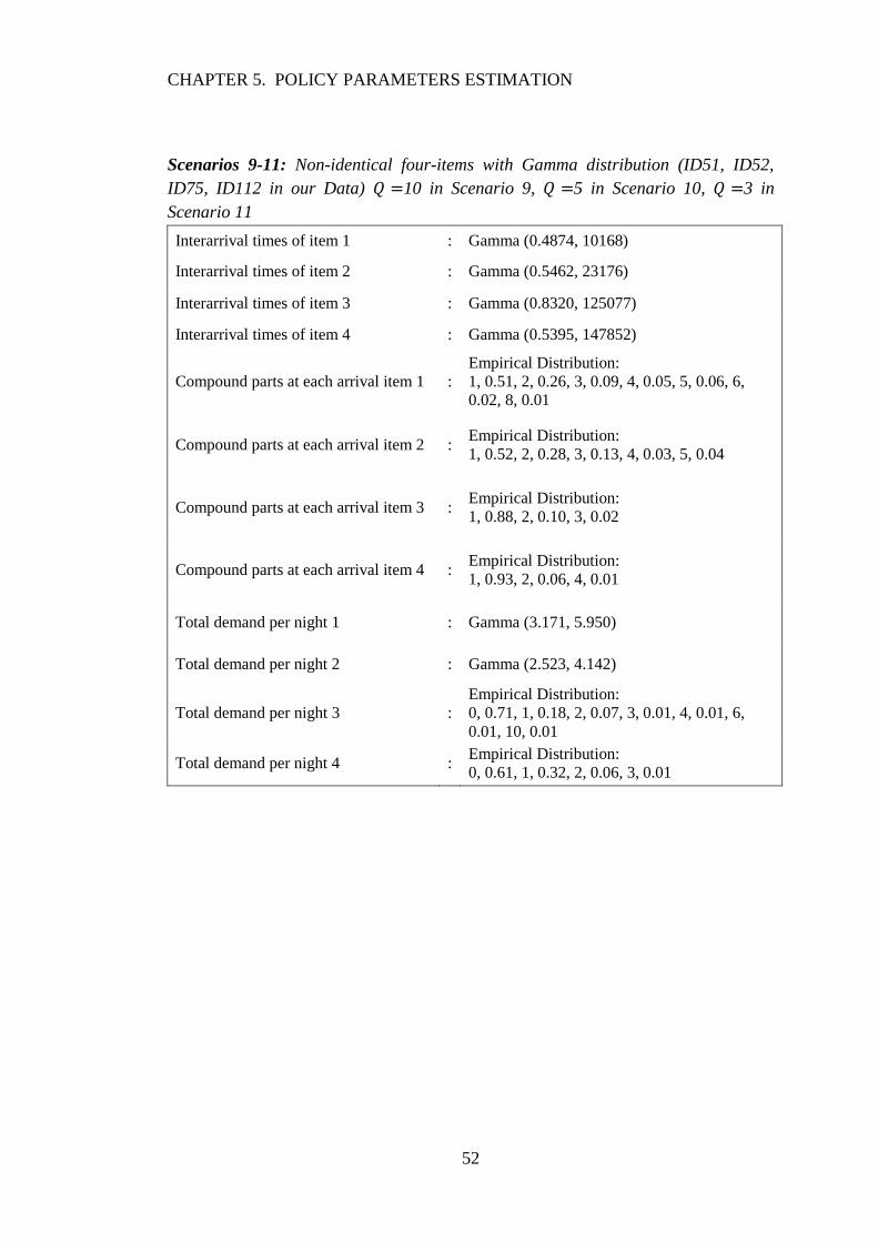
CHAPTER 5. POLICY PARAMETERS ESTIMATION
52
Scenarios 9-11: Non-identical four-items with Gamma distribution (ID51, ID52,
ID75, ID112 in our Data) 10 in Scenario 9, 5 in Scenario 10, 3 in
Scenario 11
Interarrival times of item 1 : Gamma (0.4874, 10168)
Interarrival times of item 2 : Gamma (0.5462, 23176)
Interarrival times of item 3 : Gamma (0.8320, 125077)
Interarrival times of item 4 : Gamma (0.5395, 147852)
Compound parts at each arrival item 1 :
Empirical Distribution:
1, 0.51, 2, 0.26, 3, 0.09, 4, 0.05, 5, 0.06, 6,
0.02, 8, 0.01
Compound parts at each arrival item 2 : Empirical Distribution:
1, 0.52, 2, 0.28, 3, 0.13, 4, 0.03, 5, 0.04
Compound parts at each arrival item 3 : Empirical Distribution:
1, 0.88, 2, 0.10, 3, 0.02
Compound parts at each arrival item 4 : Empirical Distribution:
1, 0.93, 2, 0.06, 4, 0.01
Total demand per night 1 : Gamma (3.171, 5.950)
Total demand per night 2 : Gamma (2.523, 4.142)
Total demand per night 3 :
Empirical Distribution:
0, 0.71, 1, 0.18, 2, 0.07, 3, 0.01, 4, 0.01, 6,
0.01, 10, 0.01
Total demand per night 4 : Empirical Distribution:
0, 0.61, 1, 0.32, 2, 0.06, 3, 0.01

CHAPTER 5. POLICY PARAMETERS ESTIMATION
53
Table 5.1: Results for the Scenario 1
Calculated Service
Levels for values values
Calculated Service
Level for values values
Day-time Realized
Service Level
Night-time Realized
Service Level Avg.
Inventory
Level per
item
# of
Replenish-
ments
during day-
time 1 2 3 4 1 2 3 4
Initial
for 98% 0.99 0.99 0.99 0.99 5 5 5 5 0.98 0.98 0.98 0.98 27 27 27 27 1.00 1.00 1.00 1.00 0.98 0.98 0.98 0.98 8.793 3.324
Optimal
for 98% 0.89 0.89 0.89 0.89 3 3 3 3 0.98 0.98 0.98 0.98 27 27 27 27 0.98 0.98 0.98 0.98 0.98 0.98 0.98 0.98 7.280 3.00
Initial
for 99% 0.99 0.99 0.99 0.99 5 5 5 5 0.99 0.99 0.99 0.99 28 28 28 28 1.00 1.00 1.00 1.00 0.99 0.99 0.99 0.99 9.019 3.167
Optimal
for 99% 0.96 0.96 0.96 0.96 4 4 4 4 0.99 0.99 0.99 0.99 28 28 28 28 0.99 0.99 0.99 0.99 0.99 0.99 0.99 0.99 7.529 2.835
Table 5.2: Results for the Scenario 2
Calculated Service
Levels for values values
Calculated Service
Level for values values
Day-time Realized
Service Level
Night-time Realized
Service Level Avg.
Inventory
Level per
item
# of
Replenish-
ments
during day-
time 1 2 3 4 1 2 3 4
Initial
for 98% 0.99 0.99 0.99 0.99 3 3 3 3 0.98 0.98 0.98 0.98 15 15 15 15 1.00 1.00 1.00 1.00 0.98 0.98 0.98 0.98 5.792 3.253
Optimal
for 98% 0.90 0.90 0.90 0.90 2 2 2 2 0.98 0.98 0.98 0.98 15 15 15 15 0.99 0.99 0.99 0.99 0.98 0.98 0.98 0.98 5.063 2.937
Initial
for 99% 0.99 0.99 0.99 0.99 3 3 3 3 0.99 0.99 0.99 0.99 16 16 16 16 1.00 1.00 1.00 1.00 0.99 0.99 0.99 0.99 6.054 2.937
Optimal
for 99% 0.90 0.90 0.90 0.90 2 2 2 2 0.99 0.99 0.99 0.99 16 16 16 16 0.99 0.99 0.99 0.99 0.99 0.99 0.99 0.99 5.373 2.622
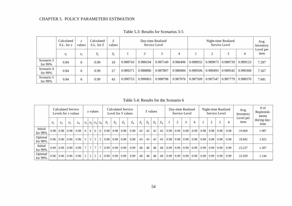
CHAPTER 5. POLICY PARAMETERS ESTIMATION
54
Table 5.3: Results for Scenarios 3-5
Calculated
S.L. for
values
Calculated
S.L. for
values
Day-time Realized
Service Level
Night-time Realized
Service Level Avg.
Inventory
Level per
item 1 2 3 4 1 2 3 4
Scenario 3
for 99% 0.84 6 0.99 18 0.988743 0.988194 0.987140 0.986496 0.988932 0.989073 0.988739 0.989123 7.397
Scenario 4
for 99% 0.84 6 0.99 27 0.989271 0.988886 0.987807 0.986984 0.989506 0.989493 0.989542 0.990368 7.567
Scenario 5
for 99% 0.84 6 0.99 43 0.990753 0.990063 0.988798 0.987976 0.987509 0.987547 0.987779 0.988370 7.681
Table 5.4: Results for the Scenario 6
Calculated Service
Levels for values values
Calculated Service
Level for values values
Day-time Realized
Service Level
Night-time Realized
Service Level Avg.
Inventory
Level per
item
# of
Replenish-
ments
during day-
time 1 2 3 4 1 2 3 4
Initial
for 98% 0.98 0.98 0.98 0.98 6 6 6 6 0.98 0.98 0.98 0.98 43 43 43 43 0.99 0.99 0.98 0.99 0.98 0.98 0.98 0.98 19.069 1.987
Optimal
for 98% 0.96 0.96 0.96 0.96 5 5 5 5 0.98 0.98 0.98 0.98 43 43 43 43 0.98 0.98 0.98 0.98 0.98 0.98 0.98 0.98 18.842 1.825
Initial
for 99% 0.99 0.99 0.99 0.99 7 7 7 7 0.99 0.99 0.99 0.99 48 48 48 48 0.99 0.99 0.99 0.99 0.99 0.99 0.99 0.99 23.237 1.387
Optimal
for 99% 0.96 0.96 0.96 0.96 5 5 5 5 0.99 0.99 0.99 0.99 48 48 48 48 0.99 0.99 0.99 0.99 0.99 0.99 0.99 0.99 22.929 1.144

CHAPTER 5. POLICY PARAMETERS ESTIMATION
55
Table 5.5: Results for the Scenario 7
Calculated Service
Levels for values values
Calculated Service
Level for values values
Day-time Realized
Service Level
Night-time Realized
Service Level Avg.
Inventory
Level per
item
# of
Replenish-
ments
during day-
time 1 2 3 4 1 2 3 4
Initial
for 98% 0.98 0.98 0.98 0.98 4 4 4 4 0.98 0.98 0.98 0.98 26 26 26 26 1.00 0.99 1.00 1.00 0.98 0.98 0.98 0.98 14.393 0.809
Optimal
for 98% 0.56 0.56 0.56 0.56 1 1 1 1 0.98 0.98 0.98 0.98 26 26 26 26 0.98 0.98 0.98 0.98 0.98 0.98 0.98 0.98 13.924 0.501
Initial
for 99% 1.00 1.00 1.00 1.00 5 5 5 5 0.99 0.99 0.99 0.99 28 28 28 28 1.00 1.00 1.00 1.00 0.99 0.99 0.99 0.99 16.214 0.699
Optimal
for 99% 0.83 0.83 0.83 0.83 2 2 2 2 0.99 0.99 0.99 0.99 28 28 28 28 0.99 0.99 0.99 0.99 0.99 0.99 0.99 0.99 15.799 0.422
Table 5.6: Results for the Scenario 8
Calculated Service
Levels for values values
Calculated Service
Level for values values
Day-time Realized
Service Level
Night-time Realized
Service Level Avg.
Inventory
Level per
item
# of
Replenish-
ments
during day-
time 1 2 3 4 1 2 3 4
Initial
for 98% 0.99 0.99 0.99 0.99 5 3 2 2 0.98 0.98 0.99 0.99 27 15 4 3 1.00 1.00 1.00 1.00 0.99 0.98 1.00 1.00 7.029 3.134
Optimal
for 98% 0.96 0.63 0.00 0.00 4 1 0 0 0.98 0.98 0.99 0.99 27 15 4 3 0.99 0.98 1.00 1.00 0.99 0.98 1.00 1.00 5.489 2.845
Initial
for 99% 0.99 0.99 0.99 0.99 5 3 2 2 0.99 0.99 0.99 1.00 28 16 4 3 1.00 1.00 1.00 1.00 0.99 0.99 1.00 1.00 7.138 2.941
Optimal
for 99% 0.96 0.90 0.00 0.00 4 2 0 0 0.99 0.99 0.99 1.00 28 16 4 3 0.99 0.99 1.00 1.00 0.99 0.99 1.00 1.00 5.769 2.743

CHAPTER 5. POLICY PARAMETERS ESTIMATION
56
Table 5.7: Results for the Scenario 9
Calculated Service
Levels for values values
Calculated Service
Level for values values
Day-time Realized
Service Level
Night-time Realized
Service Level Avg.
Inventory
Level per
item
# of
Replenish-
ments
during day-
time 1 2 3 4 1 2 3 4
Initial
for 98% 0.98 0.98 1.00 1.00 6 4 1 1 0.98 0.98 0.98 0.98 43 26 9 3 0.98 1.00 1.00 1.00 0.98 0.98 0.98 1.00 12.068 0.795
Optimal
for 98% 0.96 0.56 0.00 0.00 5 1 0 0 0.98 0.98 0.98 0.98 43 26 9 3 0.98 0.98 1.00 0.99 0.98 0.98 0.98 1.00 11.604 0.661
Initial
for 99% 0.99 1.00 1.00 1.00 7 5 1 1 0.99 0.99 1.00 0.99 48 28 10 4 0.99 0.99 1.00 1.00 0.99 0.99 1.00 1.00 13.724 0.594
Optimal
for 99% 0.96 0.56 0.00 0.00 5 1 0 0 0.99 0.99 1.00 0.99 48 28 10 4 0.99 0.99 1.00 0.99 0.99 0.99 1.00 1.00 13.253 0.436
Table 5.8: Results for Scenarios 10 and 11 where and
Calculated Service
Levels for values values
Calculated Service
Level for values values
Day-time Realized
Service Level
Night-time Realized
Service Level Avg.
Inventory
Level per
item
# of
Replenish-
ments
during day-
time 1 2 3 4 1 2 3 4
Optimal
for 99%
0.98 0.83 0.00 0.00 6 2 0 0 0.99 0.99 1.00 0.99 48 28 10 4 0.99 0.99 1.00 0.99 0.99 0.99 1.00 1.00 12.767 0.721
Optimal
for 99%
0.99 0.83 0.00 1.00 7 2 0 1 0.99 0.99 1.00 0.99 48 28 10 4 0.99 0.99 1.00 1.00 0.99 0.99 1.00 1.00 12.765 1.195
CHAPTER 5 POLICY PARAMETERS ESTIMATION
57
To sum up, in this chapter we analyze our proposed inventory control policy
under different scenarios by simulating the system in Arena. Firstly,
we show that the values that we find by using the Equation (5.1) are the exact
values, while the values that we find by using the Equation (5.2) are the
overestimated values under a specified service level target. We can also conclude
that there is actually an interaction between the items, which have different demand
rates. The item which has highest demand rate dominates the other items, and the
orders are triggered by that item in most of the cases. For this reason, this item’s
reorder level is closer to what we initially find by our calculations, while the other
items’ reorder levels tend to be much smaller. With this in mind, the search for
optimal values can be facilitated by using the following search method: For the
dominant item, start from the upper bound and decrease the value one by one, and
for the other less demanded items’ start from a much lower value than the upper
bound (even from zero) and increase the value within the range until the required
service levels are obtained. Additionally, it can be concluded that there is a negligible
effect of policy on policy, so it can be assumed that the optimal value
is not affected by the night-time demand and its control policy. Finally, it is shown
that the fixed order quantity has an effect on the reorder levels in a way that, as we
decrease the fixed order quantity, the reorder levels increase and become closer to
our initially calculated values.

58
Chapter 6
Conclusion
In this thesis, we study the inventory control problem of medical supplies that arises
in a particular hospital environment. A patient’s health is the main concern in
hospitals. Therefore, rather than minimizing the cost, we mainly focus on satisfying
the target service levels. Type 2 service level, which is the proportion of unsatisfied
demand, is taken as the performance indicator for this system. Specifically, we
consider a nursing station from which the nurses retrieve items for the patient needs.
The nursing stations can be replenished by the central warehouse at anytime during
day-time by using capacitated porter carts, but there cannot be any replenishment
during night-time since the central warehouse is closed at that period of time. Hence,
there are two distinct time frames (day-time and night-time) with different
replenishment characteristics. For the day-time inventory control, we can propose a
continuous review policy while for the night-time inventory control, we can only
propose a periodic review policy. With this in mind, we suggest a hybrid
policy to be used, in order to satisfy the required service levels for the day-
time and night-time.

CHAPTER 6. CONCLUSION
59
Before analyzing the system under these policies, we make a detailed data analysis of
the six-months data obtained from the nursing station. First of all, we divide the
items into three classes A, B and C according to total demand proportion of each
item within the inventory system. Then, in order to use in the numerical analysis we
obtain the components of demand distribution of each item. Demand distribution of
each item is composed of the distribution of the interarrival times, the distribution of
the compounding parts at each transaction, the distribution of the total number of
arrivals within lead time and the distribution of total demand per night. Interarrival
times are obtained by finding time between each consecutive transaction and the best
fitted distribution is chosen. The compounding parts at each transaction are also
gathered from the data and a distribution is fitted to this as well. In order to handle
the compounded distributions while finding the demand during lead time, we obtain
total number of arrivals within lead time by dividing the total daily demand to the
length of the day-time and fitting the best distribution to this data. Finally, for the
total demand per night distribution we sum up all transactions occurred during night
and fit the best distribution.
Our data analysis points out that 8% of the items constitute almost 83% of all items
under concern. Hence, even though there are 195 items in total, only 16 of them are
the most critical. Special attention should be paid to these items. According to our
classification, there are 45 B items and 134 C items. For controlling the most
important items, policy can be used; but for the C items individual
control can be adapted.
As a special case, for the single-item system we derive exact expressions, which
yield us the optimal policy parameters. However, since deriving such expressions for
the multi-item case is computationally hard, we simulate the system under different
scenarios and analyze the effect of the policy parameters on the service level targets.
By using the demand distribution components mentioned in the previous paragraph,
we can find the initially estimated values of and by considering required service
levels with different probability distributions. We use Arena for simulating the
system, and we search for optimal values by starting from the initial parameter
CHAPTER 6. CONCLUSION
60
values. Our results show that the estimation method for the parameter gives the
optimal value and overestimated values for the parameter . Note that, we set
parameter to one lead time ahead of the end of the day and parameter to the
capacity of the porter cart.
According to simulation results, it can also be concluded that policy has an
effect up to the fourth digit on the observed daytime service levels. It is also shown
that the fixed order quantity, , has an effect on the reorder levels in such a way that,
as the value of is decreased, values increase and become closer to our initially
estimated values. Moreover, simulation results indicate that there is an interaction
between the items in a system, which consists of items with various demand rates.
This interaction shows us the item with the highest demand rate dominates the less
demanded items at each joint ordering instance. For this reason, in this type of
system, the optimal values for the relatively low demanded items tend to be less,
while for items with high demand the optimal values tend to be close to our
initially estimated values.
By using the discussion above, we propose the following approach to set the policy
parameters for the problem under concern:
Classify the items as A, B and C and find the most important items. (Chapter
3)
For each selected item, obtain the interarrival times, compounding parts at
each transaction, total number of arrivals within lead time and the total
demand per night. Then fit the best distribution to each of these data.
(Chapter 4)
Estimate parameter for each item by using Equation 5.1. (Chapter 5)
Estimate for each item by using Equation 5.2. (Chapter 5)
In order to facilitate the searching process for the optimal parameter values;
search for the optimal values of , for the dominating items (in terms of
average demand) starting from the upper bound and for the other items
starting from zero. (Chapter 5)
CHAPTER 6. CONCLUSION
61
This study can be extended by implementing the policy to all of the
nursing stations and the items at all stations can also be replenished jointly. The
effects of jointly replenishing all stations need to be examined. Moreover, the effect
of this hybrid policy on the central warehouse can also be analyzed as a future
research.
62
Bibliography
[1] Axsater S. Inventory Control. Springer, 2006.
[2] Atkins D. R. and Iyogun P. P. Periodic versus can-order policies for
coordinated multi-item inventory systems. Management Science, 34 (6): 791-
796, 1988.
[3] Ankara Guven Hospital 2010. About us, accessed at http://www.guven.com.tr/
as of July 06, 2010.
[4] Balintfy J. L. On a basic class of multi-item inventory problems. Management
Science, 10 (2): 287-297, 1964.
[5] Bertsimas D., Bjarnadottir M. V., Kane M. A., Kryder J. C., Pandey R.,
Vempala S. and Wang G. Algorithmic prediction of health-care costs.
Operations Research, 56 (6): 1382-1392, 2008.
[6] Brandeau M., Sainfort F. and Pierskalla W. P. “Health care delivery: Current
problems and future challenges”. Operations Research and Health Care: A
handbook of methods and applications. Ed. Brandeau M., Sainfort F. and
Pierskalla W. P. Kluwer Academic Publishers, 2004.
[7] Burns L. R., DeGraaff R. A., Danzon P. M., Kimberly J. R., Kissick W. L., and
Pauly M. V. “The Wharton School of the health care value chain”. The health
care value chain: Producers, purchasers, and providers. Ed. R. Burns L. Wiley,
John & Sons, 2002.
[8] Cachon G. Managing a retailer’s shelf space, inventory and transportation.
Manufacturing and Service Operations Management, 3 (3): 211-229, 2001.
BIBLIOGRAPHY
63
[9] Chick S. E., Mamani H. and Simchi-Levi D. Supply chain coordination and
influenza vaccination. Operations Research, 56 (6): 1493-1506, 2008.
[10] Daskin M. S. and Dean L. K. “Location of health care facilities.” Operations
Research and Health Care: A handbook of methods and applications. Ed.
Brandeau M., Sainfort F. and Pierskalla W. P. Kluwer Academic Publishers,
2004.
[11] DeScioli D. T. and Byrnes J. L. S. Differentiating the hospital supply chain for
enhanced performance. Massachussetts Institute of Technology, 2005.
[12] Fung R.Y.K., Ma X. and Lau H.C.W. (T,S) policy for coordinated inventory
replenishment systems under compound Poisson demands. Production
Planning and Control, 12 (6): 575-583, 2001.
[13] Green L. “Capacity planning and management in hospitals.” Operations
Research and Health Care: A handbook of methods and applications. Ed.
Brandeau M., Sainfort F. and Pierskalla W. P. Kluwer Academic Publishers,
2004.
[14] Henderson S. G. and Mason A. J. “Ambulance service planning: Simulation
and data visualisation.” Operations Research and Health Care: A handbook of
methods and applications. Ed. Brandeau M., Sainfort F. and Pierskalla W. P.
Kluwer Academic Publishers, 2004.
[15] Kumar A., Ozdamar L., and Zhang C. N. Supply chain redesign in the
healthcare industry of Singapore. Supply Chain Management: An International
Journal, 13 (2): 95-103, 2008.
[16] Lee C. P., Chertow G. M. and Zenios S. A. Optimal initiation and management
of dialysis theraphy. Operations Research, 56 (6): 1428-1449, 2008.
[17] Lee E. K. and Zaider M. Operations research advances cancer therapeutics.
Interfaces, 38 (1): 5-25, 2008.
[18] Little J. and Coughlan B. Optimal inventory policy within hospital space
constraints. Health Care Management Science, 11 (2): 177-183, 2008.
[19] Maillart L. M., Ivy J. S., Ransom S. and Diehl K. Assessing dynamic breast
cancer screening policies. Operations Research, 56 (6): 1411-1427, 2008.

BIBLIOGRAPHY
64
[20] Nicholson L., Vakharia A. J. and Erenguc S. S. Outsourcing inventory
management decisions in healthcare: Models and application. European
Journal of Operational Research, 154 (1): 271-290, 2004.
[21] Nielsen C. and Larsen C. An analytical study of the Q(s,S) policy applied to
the joint replenishment problem. European Journal of Operational
Research, 163 (3): 721-732, 2005.
[22] Ozkaya B., Gurler U. and Berk E. The stochastic joint replenishment problem:
A new policy, analysis and insights. Naval Research Logistics, 53 (6): 525-
546, 2006.
[23] Pantumsinchai P. A comparison of three joint ordering policies. Decision
Sciences, 23: 111-127, 1992.
[24] Renberg B. and Planche R. Un mode´le pour la gestion simultane´e des n
articles d’un stock. Rev Franc Inform Rech Ope´r, 6: 47-59, 1967.
[25] Rivard-Royer H., Landry S. and Beaulieu M. Hybrid stockless: a case study:
Lessons for health-care supply chain integration. International Journal of
Operations and Production Management, 22 (4): 412-424, 2002.
[26] Satir, A. and Cengiz, D. Medicinal Inventory Control in a University Health
Centre. Journal of the Operational Research Society, 38: 387-395, 1987.
[27] Tanrikulu M. M., Sen A. and Alp O. A joint replenishment policy with
individual control and constant size orders. International Journal of Production
Research, 48 (14): 1-19, 2009.
[28] Viswanathan S. Periodic review (s,S) policies for joint replenishment inventory
systems. Management Science, 43 (10): 1447-1454, 1997.
65
Appendix A
The Detailed Information of the Items
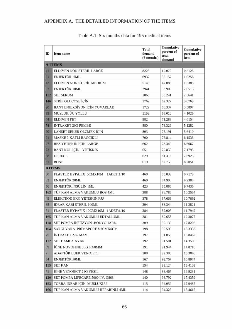
APPENDIX A. THE DETAILED INFORMATION OF THE ITEMS
66
Table A.1: Six months data for 195 medical items
ID Item name
Total
demand
(6 months)
Cumulative
percent of
total
demand
Cumulative
percent of
item
A ITEMS
41 ELDİVEN NON STERİL LARGE 8223 19.070 0.5128
51 ENJEKTÖR 5ML 6937 35.157 1.0256
42 ELDİVEN NON STERİL MEDIUM 5145 47.088 1.5385
52 ENJEKTÖR 10ML 2941 53.909 2.0513
122 SET SERUM 1868 58.241 2.5641
146 STRİP GLUCOSE İÇİN 1762 62.327 3.0769
20 BANT ENJEKSİYON İÇİN YUVARLAK 1729 66.337 3.5897
95 MUSLUK ÜÇ YOLLU 1153 69.010 4.1026
44 ELDİVEN PET 982 71.288 4.6154
74 İNTRAKET 20G PEMBE 880 73.329 5.1282
90 LANSET ŞEKER ÖLÇMEK İÇİN 803 75.191 5.6410
91 MASKE 3 KATLI BAĞCIKLI 700 76.814 6.1538
27 BEZ YETİŞKİN İÇİN LARGE 662 78.349 6.6667
22 BANT KOL İÇİN YETİŞKİN 651 79.859 7.1795
38 DERECE 629 81.318 7.6923
31 BONE 619 82.753 8.2051
B ITEMS
60 FLASTER HYPAFIX 5CMX10M 1ADET:1/10 468 83.839 8.7179
53 ENJEKTÖR 20ML 460 84.905 9.2308
56 ENJEKTÖR İNSÜLİN 1ML 423 85.886 9.7436
163 TÜP KAN ALMA VAKUMLU BOŞ 4ML 388 86.786 10.2564
49 ELEKTROD EKG YETİŞKİN F55 378 87.663 10.7692
65 İDRAR KABI STERİL 100ML 294 88.344 11.2821
61 FLASTER HYPAFIX 10CMX10M 1ADET:1/10 284 89.003 11.7949
165 TÜP KAN ALMA VAKUMLU EDTALI 3ML 281 89.655 12.3077
118 SET POMPA İNFÜZYON -BODYGUARD- 209 90.139 12.8205
104 SARGI YARA PRİMAPORE 8.3CMX6CM 198 90.599 13.3333
75 İNTRAKET 22G MAVİ 197 91.055 13.8462
112 SET DAMLA AYAR 192 91.501 14.3590
69 İĞNE NOVOFINE 30G 0.3/8MM 191 91.944 14.8718
2 ADAPTÖR LUER VENOJECT 188 92.380 15.3846
54 ENJEKTÖR 50ML 167 92.767 15.8974
115 SET KAN 154 93.124 16.4103
71 İĞNE VENOJECT 21G YEŞİL 148 93.467 16.9231
120 SET POMPA LIFECARE 5000 I.V. G868 140 93.792 17.4359
153 TORBA İDRAR İÇİN MUSLUKLU 115 94.059 17.9487
166 TÜP KAN ALMA VAKUMLU HEPARİNLİ 4ML 114 94.323 18.4615
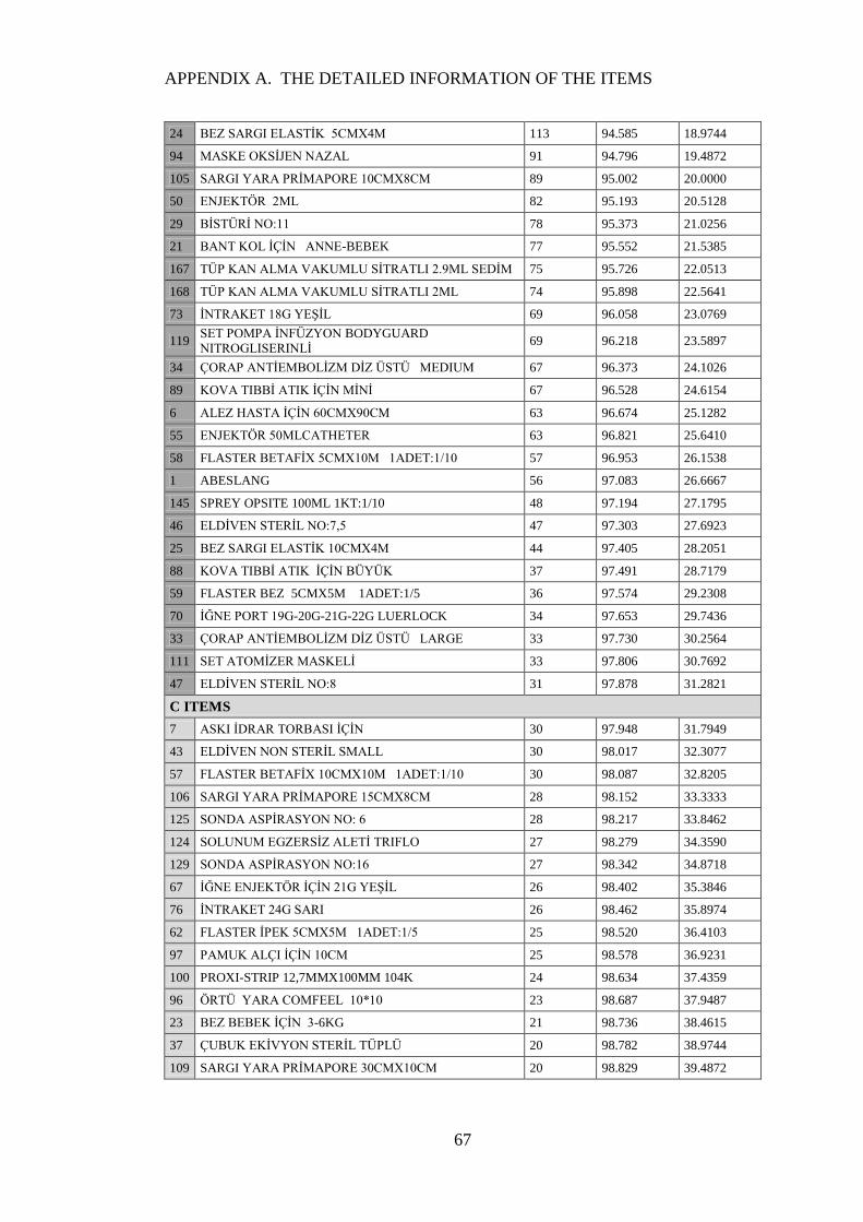
APPENDIX A. THE DETAILED INFORMATION OF THE ITEMS
67
24 BEZ SARGI ELASTİK 5CMX4M 113 94.585 18.9744
94 MASKE OKSİJEN NAZAL 91 94.796 19.4872
105 SARGI YARA PRİMAPORE 10CMX8CM 89 95.002 20.0000
50 ENJEKTÖR 2ML 82 95.193 20.5128
29 BİSTÜRİ NO:11 78 95.373 21.0256
21 BANT KOL İÇİN ANNE-BEBEK 77 95.552 21.5385
167 TÜP KAN ALMA VAKUMLU SİTRATLI 2.9ML SEDİM 75 95.726 22.0513
168 TÜP KAN ALMA VAKUMLU SİTRATLI 2ML 74 95.898 22.5641
73 İNTRAKET 18G YEŞİL 69 96.058 23.0769
119 SET POMPA İNFÜZYON BODYGUARD
NITROGLISERINLİ 69 96.218 23.5897
34 ÇORAP ANTİEMBOLİZM DİZ ÜSTÜ MEDIUM 67 96.373 24.1026
89 KOVA TIBBİ ATIK İÇİN MİNİ 67 96.528 24.6154
6 ALEZ HASTA İÇİN 60CMX90CM 63 96.674 25.1282
55 ENJEKTÖR 50MLCATHETER 63 96.821 25.6410
58 FLASTER BETAFİX 5CMX10M 1ADET:1/10 57 96.953 26.1538
1 ABESLANG 56 97.083 26.6667
145 SPREY OPSITE 100ML 1KT:1/10 48 97.194 27.1795
46 ELDİVEN STERİL NO:7,5 47 97.303 27.6923
25 BEZ SARGI ELASTİK 10CMX4M 44 97.405 28.2051
88 KOVA TIBBİ ATIK İÇİN BÜYÜK 37 97.491 28.7179
59 FLASTER BEZ 5CMX5M 1ADET:1/5 36 97.574 29.2308
70 İĞNE PORT 19G-20G-21G-22G LUERLOCK 34 97.653 29.7436
33 ÇORAP ANTİEMBOLİZM DİZ ÜSTÜ LARGE 33 97.730 30.2564
111 SET ATOMİZER MASKELİ 33 97.806 30.7692
47 ELDİVEN STERİL NO:8 31 97.878 31.2821
C ITEMS
7 ASKI İDRAR TORBASI İÇİN 30 97.948 31.7949
43 ELDİVEN NON STERİL SMALL 30 98.017 32.3077
57 FLASTER BETAFİX 10CMX10M 1ADET:1/10 30 98.087 32.8205
106 SARGI YARA PRİMAPORE 15CMX8CM 28 98.152 33.3333
125 SONDA ASPİRASYON NO: 6 28 98.217 33.8462
124 SOLUNUM EGZERSİZ ALETİ TRIFLO 27 98.279 34.3590
129 SONDA ASPİRASYON NO:16 27 98.342 34.8718
67 İĞNE ENJEKTÖR İÇİN 21G YEŞİL 26 98.402 35.3846
76 İNTRAKET 24G SARI 26 98.462 35.8974
62 FLASTER İPEK 5CMX5M 1ADET:1/5 25 98.520 36.4103
97 PAMUK ALÇI İÇİN 10CM 25 98.578 36.9231
100 PROXI-STRIP 12,7MMX100MM 104K 24 98.634 37.4359
96 ÖRTÜ YARA COMFEEL 10*10 23 98.687 37.9487
23 BEZ BEBEK İÇİN 3-6KG 21 98.736 38.4615
37 ÇUBUK EKİVYON STERİL TÜPLÜ 20 98.782 38.9744
109 SARGI YARA PRİMAPORE 30CMX10CM 20 98.829 39.4872
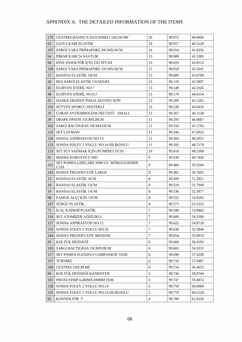
APPENDIX A. THE DETAILED INFORMATION OF THE ITEMS
68
170 UZATMA BASINCA DAYANIKLI 145CM MF 20 98.875 40.0000
63 GAİTA KABI PLASTİK 18 98.917 40.5128
107 SARGI YARA PRİMAPORE 20CMX10CM 16 98.954 41.0256
64 İDRAR KABI 24 SAATLİK 15 98.989 41.5385
68 İĞNE ENJEKTÖR İÇİN 22G SİYAH 15 99.024 42.0513
108 SARGI YARA PRİMAPORE 25CMX10CM 15 99.058 42.5641
17 BANDAJ ELASTİK 10CM 13 99.089 43.0769
26 BEZ SARGI ELASTİK 15CMX4M 13 99.119 43.5897
45 ELDİVEN STERİL NO:7 13 99.149 44.1026
48 ELDİVEN STERİL NO:8,5 13 99.179 44.6154
93 MASKE OKSİJEN İNHALASYONU İÇİN 13 99.209 45.1282
150 SÜTYEN SPORCU DESTEKLİ 13 99.239 45.6410
35 ÇORAP ANTİEMBOLİZM DİZ ÜSTÜ SMALL 12 99.267 46.1538
39 DRAPE OPSITE 15CMX28CM 11 99.293 46.6667
102 SARGI BACTIGRAS 10CMX10CM 11 99.318 47.1795
116 SET LAVMAN 11 99.344 47.6923
128 SONDA ASPİRASYON NO:14 11 99.369 48.2051
133 SONDA FOLEY 2 YOLLU NO:16 SİLİKONLU 11 99.395 48.7179
123 SET SÜT SAĞMAK İÇİN (PUMPSET ECO) 10 99.418 49.2308
92 MASKE KORUYUCU N95 9 99.439 49.7436
121 SET POMPA LIFECARE 5000 I.V. NITROGLISERIN
L218 9 99.460 50.2564
143 SONDA PREZERVATİF LARGE 9 99.481 50.7692
15 BANDAJ ELASTİK 6CM 8 99.499 51.2821
18 BANDAJ ELASTİK 12CM 8 99.518 51.7949
19 BANDAJ ELASTİK 15CM 8 99.536 52.3077
98 PAMUK ALÇI İÇİN 15CM 8 99.555 52.8205
147 SÜRGÜ PLASTİK 8 99.573 53.3333
72 İLAÇ KADEHİ PLASTİK 7 99.590 53.8462
110 SET ATOMİZER AĞIZLIKLI 7 99.606 54.3590
127 SONDA ASPİRASYON NO:12 7 99.622 54.8718
132 SONDA FOLEY 2 YOLLU NO:16 7 99.638 55.3846
144 SONDA PREZERVATİF MEDIUM 7 99.654 55.8974
83 KOLTUK DEĞNEĞİ 6 99.668 56.4103
103 SARGI BACTIGRAS 15CMX20CM 6 99.682 56.9231
117 SET POMPA FLEXIFLO COMPANION G938 6 99.696 57.4359
157 TURNİKE 6 99.710 57.9487
169 UZATMA 145CM MF 6 99.724 58.4615
84 KOLTUK DEĞNEĞİ KANEDYEN 5 99.736 58.9744
101 PROXI-STRIP 6,4MMX100MM 103K 5 99.747 59.4872
130 SONDA FOLEY 2 YOLLU NO:14 5 99.759 60.0000
135 SONDA FOLEY 2 YOLLU NO:18 SİLİKONLU 5 99.770 60.5128
85 KONNEKTÖR T 4 99.780 61.0256
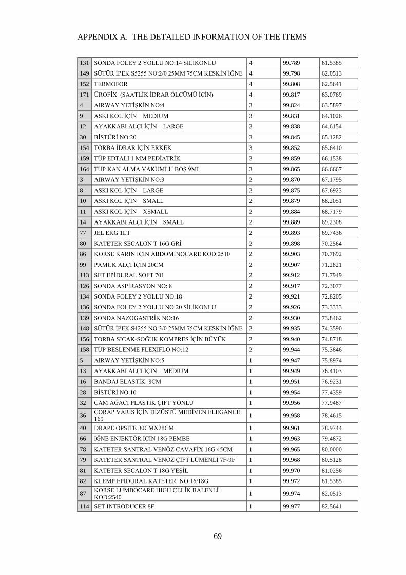
APPENDIX A. THE DETAILED INFORMATION OF THE ITEMS
69
131 SONDA FOLEY 2 YOLLU NO:14 SİLİKONLU 4 99.789 61.5385
149 SÜTÜR İPEK S5255 NO:2/0 25MM 75CM KESKİN İĞNE 4 99.798 62.0513
152 TERMOFOR 4 99.808 62.5641
171 ÜROFİX (SAATLİK İDRAR ÖLÇÜMÜ İÇİN) 4 99.817 63.0769
4 AIRWAY YETİŞKİN NO:4 3 99.824 63.5897
9 ASKI KOL İÇİN MEDIUM 3 99.831 64.1026
12 AYAKKABI ALÇI İÇİN LARGE 3 99.838 64.6154
30 BİSTÜRİ NO:20 3 99.845 65.1282
154 TORBA İDRAR İÇİN ERKEK 3 99.852 65.6410
159 TÜP EDTALI 1 MM PEDİATRİK 3 99.859 66.1538
164 TÜP KAN ALMA VAKUMLU BOŞ 9ML 3 99.865 66.6667
3 AIRWAY YETİŞKİN NO:3 2 99.870 67.1795
8 ASKI KOL İÇİN LARGE 2 99.875 67.6923
10 ASKI KOL İÇİN SMALL 2 99.879 68.2051
11 ASKI KOL İÇİN XSMALL 2 99.884 68.7179
14 AYAKKABI ALÇI İÇİN SMALL 2 99.889 69.2308
77 JEL EKG 1LT 2 99.893 69.7436
80 KATETER SECALON T 16G GRİ 2 99.898 70.2564
86 KORSE KARIN İÇİN ABDOMİNOCARE KOD:2510 2 99.903 70.7692
99 PAMUK ALÇI İÇİN 20CM 2 99.907 71.2821
113 SET EPİDURAL SOFT 701 2 99.912 71.7949
126 SONDA ASPİRASYON NO: 8 2 99.917 72.3077
134 SONDA FOLEY 2 YOLLU NO:18 2 99.921 72.8205
136 SONDA FOLEY 2 YOLLU NO:20 SİLİKONLU 2 99.926 73.3333
139 SONDA NAZOGASTRİK NO:16 2 99.930 73.8462
148 SÜTÜR İPEK S4255 NO:3/0 25MM 75CM KESKİN İĞNE 2 99.935 74.3590
156 TORBA SICAK-SOĞUK KOMPRES İÇİN BÜYÜK 2 99.940 74.8718
158 TÜP BESLENME FLEXIFLO NO:12 2 99.944 75.3846
5 AIRWAY YETİŞKİN NO:5 1 99.947 75.8974
13 AYAKKABI ALÇI İÇİN MEDIUM 1 99.949 76.4103
16 BANDAJ ELASTİK 8CM 1 99.951 76.9231
28 BİSTÜRİ NO:10 1 99.954 77.4359
32 ÇAM AĞACI PLASTİK ÇİFT YÖNLÜ 1 99.956 77.9487
36 ÇORAP VARİS İÇİN DİZÜSTÜ MEDİVEN ELEGANCE
169 1 99.958 78.4615
40 DRAPE OPSITE 30CMX28CM 1 99.961 78.9744
66 İĞNE ENJEKTÖR İÇİN 18G PEMBE 1 99.963 79.4872
78 KATETER SANTRAL VENÖZ CAVAFİX 16G 45CM 1 99.965 80.0000
79 KATETER SANTRAL VENÖZ ÇİFT LÜMENLİ 7F-9F 1 99.968 80.5128
81 KATETER SECALON T 18G YEŞİL 1 99.970 81.0256
82 KLEMP EPİDURAL KATETER NO:16/18G 1 99.972 81.5385
87 KORSE LUMBOCARE HIGH ÇELİK BALENLİ
KOD:2540 1 99.974 82.0513
114 SET INTRODUCER 8F 1 99.977 82.5641
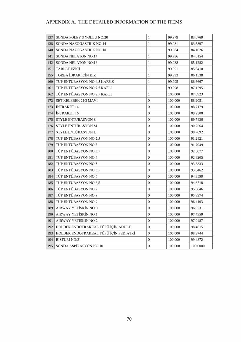
APPENDIX A. THE DETAILED INFORMATION OF THE ITEMS
70
137 SONDA FOLEY 3 YOLLU NO:20 1 99.979 83.0769
138 SONDA NAZOGASTRİK NO:14 1 99.981 83.5897
140 SONDA NAZOGASTRİK NO:18 1 99.984 84.1026
141 SONDA NELATON NO:14 1 99.986 84.6154
142 SONDA NELATON NO:16 1 99.988 85.1282
151 TABLET EZİCİ 1 99.991 85.6410
155 TORBA İDRAR İÇİN KIZ 1 99.993 86.1538
160 TÜP ENTÜBASYON NO:4,5 KAFSIZ 1 99.995 86.6667
161 TÜP ENTÜBASYON NO:7,5 KAFLI 1 99.998 87.1795
162 TÜP ENTÜBASYON NO:8,5 KAFLI 1 100.000 87.6923
172 SET KELEBEK 21G MAVİ 0 100.000 88.2051
173 İNTRAKET 14 0 100.000 88.7179
174 İNTRAKET 16 0 100.000 89.2308
175 STYLE ENTÜBASYON S 0 100.000 89.7436
176 STYLE ENTÜBASYON M 0 100.000 90.2564
177 STYLE ENTÜBASYON L 0 100.000 90.7692
178 TÜP ENTÜBASYON NO:2,5 0 100.000 91.2821
179 TÜP ENTÜBASYON NO:3 0 100.000 91.7949
180 TÜP ENTÜBASYON NO:3,5 0 100.000 92.3077
181 TÜP ENTÜBASYON NO:4 0 100.000 92.8205
182 TÜP ENTÜBASYON NO:5 0 100.000 93.3333
183 TÜP ENTÜBASYON NO:5,5 0 100.000 93.8462
184 TÜP ENTÜBASYON NO:6 0 100.000 94.3590
185 TÜP ENTÜBASYON NO:6,5 0 100.000 94.8718
186 TÜP ENTÜBASYON NO:7 0 100.000 95.3846
187 TÜP ENTÜBASYON NO:8 0 100.000 95.8974
188 TÜP ENTÜBASYON NO:9 0 100.000 96.4103
189 AIRWAY YETİŞKİN NO:0 0 100.000 96.9231
190 AIRWAY YETİŞKİN NO:1 0 100.000 97.4359
191 AIRWAY YETİŞKİN NO:2 0 100.000 97.9487
192 HOLDER ENDOTRAKEAL TÜPÜ İÇİN ADULT 0 100.000 98.4615
193 HOLDER ENDOTRAKEAL TÜPÜ İÇİN PEDİATRİ 0 100.000 98.9744
194 BİSTÜRİ NO:21 0 100.000 99.4872
195 SONDA ASPİRASYON NO:10 0 100.000 100.0000

APPENDIX A. THE DETAILED INFORMATION OF THE ITEMS
71
Table A.2: Descriptive statistics of some items
ID Mean Standard
Deviation Variance
Coefficient
of Variance Median Skewness
41 42.39 32.88 1080.86 77.56 34.5 2.21
51 35.94 20.6 424.16 57.3 31 1.6
42 30.26 24.22 586.44 80.02 25 2.01
52 15.73 8.646 74.759 54.98 14 0.76
122 9.629 5.503 30.286 57.15 9 0.79
146 10.37 7.858 61.748 75.81 8 1.06
20 9.005 4.933 24.33 54.77 8 0.87
95 6.199 3.756 14.106 60.59 5 1.41
44 11.16 13.59 184.78 121.81 7.5 4.2
74 5 3.576 12.789 71.52 4 1.37
90 4.751 3.047 9.283 64.12 4 0.84
91 7.61 11.76 138.2 154.5 3 2.89
27 5.213 4.027 16.216 77.25 4 1.23
22 4.043 2.871 8.242 71 4 2.08
38 3.722 2.249 5.059 60.43 3 0.78
31 3.893 2.863 8.197 73.54 3 1.8
60 3.467 3.325 11.057 95.92 2 2.38
53 3.046 1.964 3.858 64.47 3 1.39
56 3.881 3.011 9.069 77.6 3 1.94
163 2.504 1.9 3.61 75.89 2 1.93
49 5.25 3.201 10.246 60.97 4 2.58
65 1.534 1.068 1.141 69.63 1 2.44
61 2.757 1.86 3.46 67.46 2 1.51
165 2.178 1.518 2.304 69.68 2 1.69
118 1.833 0.9769 0.9543 53.28 2 1.04
104 2.676 1.851 3.428 69.19 2 0.87
75 1.791 1.382 1.91 77.17 1 3.51
112 1.67 0.915 0.8372 54.8 1 1.48
69 2.513 1.447 2.093 57.57 2 1.34
2 2 1.503 2.258 75.13 1 1.9
54 1.856 1.204 1.451 64.91 1 2.14
115 1.812 1.239 1.536 68.4 1 2.41
71 1.701 1.101 1.212 64.71 1 2.12
120 1.296 0.568 0.3226 43.82 1 1.79
153 1.797 1.287 1.656 71.63 1 2.33
166 1.81 1.105 1.221 61.07 1 1.95
24 1.592 0.935 0.874 58.73 1 1.99
94 1.358 0.6675 0.4455 49.14 1 1.96
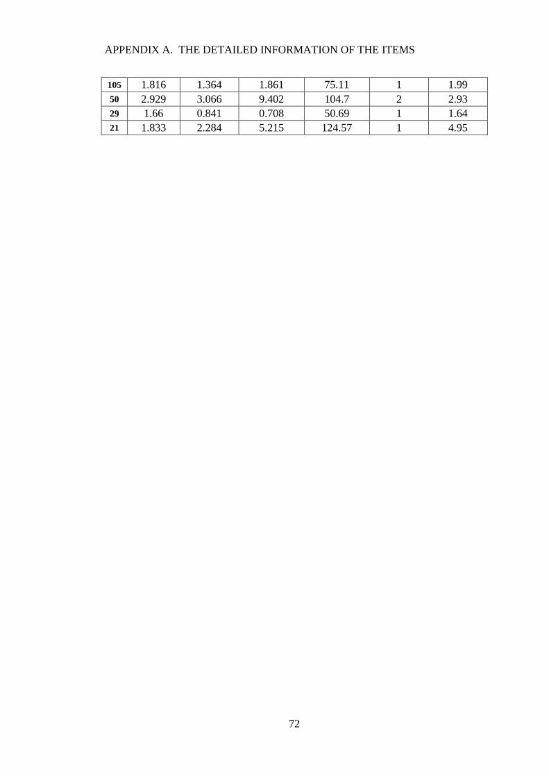
APPENDIX A. THE DETAILED INFORMATION OF THE ITEMS
72
105 1.816 1.364 1.861 75.11 1 1.99
50 2.929 3.066 9.402 104.7 2 2.93
29 1.66 0.841 0.708 50.69 1 1.64
21 1.833 2.284 5.215 124.57 1 4.95

73
Appendix B
Daily Demand Distributions of Some
Items

APPENDIX B. DAILY DEMAND DISTRIBUTIONS OF SOME ITEMS
74
1501209060300
40
30
20
10
0
Daily Demand
Fre
qu
en
cy
Shape 1.517
Scale 19.95
N 170
Gamma
Daily Demand Histogram ID42
Figure B.1: Daily Demand Distributions for the item ID42
140120100806040200
50
40
30
20
10
0
Daily Demand
Fre
qu
en
cy
Shape 3.234
Scale 11.12
N 193
Gamma
Daily Demand Histogram ID51
Figure B.2: Daily Demand Distributions for the item ID51

APPENDIX B. DAILY DEMAND DISTRIBUTIONS OF SOME ITEMS
75
2101801501209060300
60
50
40
30
20
10
0
Daily Demand
Fre
qu
en
cy
Shape 1.940
Scale 21.84
N 194
Gamma
Daily Demand Histogram ID41
Figure B.3: Daily Demand Distributions for the item ID41
363024181260
25
20
15
10
5
0
Daily Demand
Fre
qu
en
cy
Shape 1.659
Scale 6.248
N 170
Gamma
Daily Demand Histogram ID146
Figure B.4: Daily Demand Distributions for the item ID146
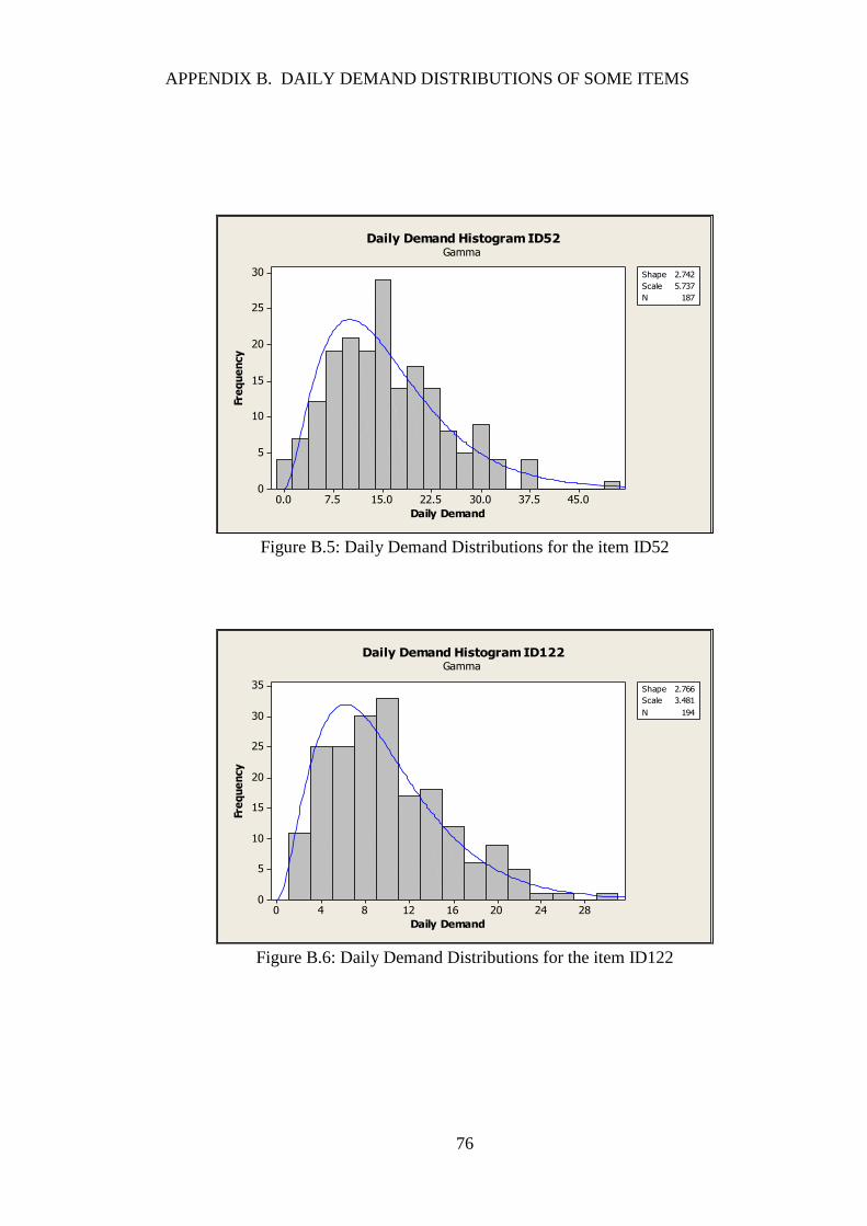
APPENDIX B. DAILY DEMAND DISTRIBUTIONS OF SOME ITEMS
76
45.037.530.022.515.07.50.0
30
25
20
15
10
5
0
Daily Demand
Fre
qu
en
cy
Shape 2.742
Scale 5.737
N 187
Gamma
Daily Demand Histogram ID52
Figure B.5: Daily Demand Distributions for the item ID52
2824201612840
35
30
25
20
15
10
5
0
Daily Demand
Fre
qu
en
cy
Shape 2.766
Scale 3.481
N 194
Gamma
Daily Demand Histogram ID122
Figure B.6: Daily Demand Distributions for the item ID122