Full Terms & Conditions of access and use can be found athttps://www.tandfonline.com/action/journalInformation?journalCode=tscf20

Supply Chain Forum: An International Journal

ISSN: (Print) (Online) Journal homepage: https://www.tandfonline.com/loi/tscf20

A hybrid demand forecasting model forgreater forecasting accuracy: the case of thepharmaceutical industry

Raheel Siddiqui, Muhammad Azmat, Shehzad Ahmed & Sebastian Kummer

To cite this article: Raheel Siddiqui, Muhammad Azmat, Shehzad Ahmed & SebastianKummer (2021): A hybrid demand forecasting model for greater forecasting accuracy: thecase of the pharmaceutical industry, Supply Chain Forum: An International Journal, DOI:10.1080/16258312.2021.1967081

To link to this article: https://doi.org/10.1080/16258312.2021.1967081

© 2021 The Author(s). Published by InformaUK Limited, trading as Taylor & FrancisGroup.

View supplementary material

Published online: 05 Sep 2021. Submit your article to this journal

Article views: 364 View related articles

View Crossmark data

A hybrid demand forecasting model for greater forecasting accuracy: the case of the pharmaceutical industryRaheel Siddiqui a, Muhammad Azmat b, Shehzad Ahmed c and Sebastian Kummerd,e

aDepartment of Management Sciences, Mohammad Ali Jinnah University, Karachi, Sindh, Pakistan; bCollege of Engineering and Physical Sciences, Department of Engineering Systems and Supply Chain Management (ESSCM), Aston University, UK; cSchool of Business and Creative Industries, University of the West of Scotland, Paisley, Scotland, UK; dSchool of Management, Department of Logistics Management, Jilin University, Changchun, Jilin, China; eInstitute for Transport and Logistics Management, Vienna University of Economics and Business, Vienna, Austria

ABSTRACTIn the era of modern technology, the competitive paradigm among organisations is changing at an unprecedented rate. New success measures are applied to the organisation’s supply chain performance to outperform the competition. However, this lead can only be obtained and sustained if the organisation has an effective and efficient supply chain and an appropriate forecasting technique. Thus, this study presents the demand-forecasting model, i.e., a good fit for the pharmaceutical sector, and shows promising results. Through this study, it is observed that combining forecasting algorithms can result in greater forecasting accuracies. Therefore, a combined forecasting technique ARIMA-HW hybrid1 i.e. (ARHOW) combines the Autoregressive Integrated Moving Average and Holt’ s-Winter model. The empirical findings confirm that ARHOW performs better than widely used forecasting techniques ARIMA, Holts Winter, ETS and Theta. The results of the study indicate that pharmaceutical companies can adopt this model for improved demand forecasting.

KEYWORDS Forecast; combined forecast; hybrid forecast; supply chain efficiency; demand forecasting; forecasting technique for integrated systems; pharmaceutical industry

Introduction

In the pharmaceutical industry, demand forecasting is essential for optimising and managing complex busi-ness processes (MERKURYEVA and ALEXANDER SMIRNOV 2019). Transparent and unobstructed infor-mation flow directly affects supply chain (SC) dynamics (BOONE et al. 2019; FILDES, GOODWIN, and ÖNKAL 2019). Data sharing between the purchaser and seller in the SC network has been considered useful in avoid-ing the purported bullwhip impact and enhancing SC operations (BOYCE, JOHN, and KENT 2016). ‘Recent technological developments enable designing useful forecasting models to increase supply chain manage-ment (SCM) efficiency (Habibeh Zeraati, 2019; IM, RAI, and LAMBERT 2019)’. Indeed, collecting data from sev-eral actors, such as the distributors, the healthcare providers and the customers (i.e. patients) becomes easier (SECGINLI, ERDOGAN, and MONSEN 2014). Digitisation brings companies to shift a flexible cost base, reduces the risk, and aligns the SC network with its demand forecasts (SCHNIEDERJANS, CURADO, and KHALAJHEDAYATI 2020; ZHANG and ZHANG 2018). Data collection through external and internal colla-borations that include Vendor-managed Inventory (VMI), Electronic Data Interchange (EDI), and sales operations are more accurate and drive better

forecasting results (NASIRI et al. 2020; AGOSTINO et al. 2020). However, it should be pointed out that available technologies should be appropriately explored for computing demand forecasts to increase SC efficiency (PWC 2016). WELLER and CRONE (2012) stated that data are mostly collected for demand fore-casting purposes by employing a collaborative infor-mation-sharing mechanism. From other sources like sales and operations, collaborative planning forecast-ing and replenishment and vendor managing inven-tory data help the manufacturers forecast accurately. According to Munim and Schramm (2017), the hybrid forecasting model ARIMARCH combining the Auto- Regressive Integrated Moving Average (ARIMA) and Autoregressive Conditional Heteroscedasticity (Walters and Archer) model enhances the forecasting accuracy when compared to that yield by the appli-ance of a single forecasting model.

Moreover, the Mean Absolute Percentage Error (MAPE) obtained by employing the state-of-the-art model ARIMARCH developed by Munim and Schramm (2017) has shown significant forecasting results applying model ARIMA and ARCH indepen-dently for forecasting. A combined forecasting techni-que that considers historical and current demand data records has been used to forecast demand for the

CONTACT Muhammad Azmat m.azmat@aston.ac.uk College of Engineering and Physical Sciences, Department of Engineering Systems and Supply Chain Management (ESSCM), Aston University, B4 7ET, United Kingdom.

Supplemental data for this article can be accessed here.

SUPPLY CHAIN FORUM: AN INTERNATIONAL JOURNAL https://doi.org/10.1080/16258312.2021.1967081

© 2021 The Author(s). Published by Informa UK Limited, trading as Taylor & Francis Group. This is an Open Access article distributed under the terms of the Creative Commons Attribution License (http://creativecommons.org/licenses/by/4.0/), which permits unrestricted use, distribution, and reproduction in any medium, provided the original work is properly cited.

Human Immunodeficiency Virus (HIV) diagnostics. In particular, linear extrapolation has been applied to the data of the WHO survey for demand forecasting. In contrast, the Clinton Health Access Initiative (CHAI) has been used when dealing with the historical demand of countries that fall under CHAI’s umbrella (WHO 2016). Based on the consolidated forecasting: 80% is accounted for from CHAI, and 20% are linear extrapolation. Deep learning tools can help achieve higher forecast accuracy by creating patterns in deci-sion making rather than using a single model to fore-cast demand (THOMSON et al. 2019). By combining various machine-learning models; it will help to resolve issues of warehouse forecasting. Hence, the devised method’s forecast error is less than 5% compared to predicting through a single model for forecasting methods; thus, the combined variants reveals better performance (ISLEK, S. G. O 2017).

Moreover, the stacked generalisation method developed for the decision support system reduces the error rate by 9% compared to forecasting through traditional processes like forecasting by using a model. NIKOLOPOULOS et al. (2016) worked on pharmaceuti-cals brands and generics to forecast the demand. For this instance, seven different forecasting techniques have been applied as deep learning tools to analyse the past 21 years’ data set. The empirical result exhibits that both ARIMA and Holts Winter combined produces a more accurate forecast in a shorter period. In con-trast, the Naïve technique has a more significant fore-casting result for a period of 2 to 5 years.

Literature Review

Practitioners usually face significant challenges in under-standing and applying forecasts due to the lack of avail-able related literature review. Significant savings, improved communication, better working practices, and enhance forecast accuracy can be achieved by employing a sound decision support system for forecasting purposes (FILDES and GOODWIN 2020; DURAND 2003). For this instance, Enterprise Resource Planning System (ERP) is used to get accurate real-time information and forecast computed results by applying the available models in the ERP systems (JanePHILLIPS and NIKOLOPOULOS 2019). The following systems have been studied thoroughly, the available functionality in the ERP system for demand forecasting. Table 1 indicates seven ERP systems that are mostly used for this purpose.

Demand Forecasting and Integrating Systems

Furthermore, by deploying an ERP system and using demand forecasting functionality appropriately with accurate data, an organisation would reduce inventory levels (TIWARI 2020; ERKAYMAN 2018). Higher inven-tory levels are a significant risk in the SC because it

freezes the capital and holds inventory cost that leads a company towards bankruptcy (CRONE and D. S 2013). On the other hand, integrated systems with suitable models enable manufacturers to decrease the gap between actual and forecast demand; thus results in competitive advantage (HININGS, GEGENHUBER, and GREENWOOD 2018; AYTAC and WU 2017). Moreover, users’ involvement in the forecasting model’s development may increase the model’s probability of success. On the one hand, the integrated system allows seamless information synchronisation between departments resulting in better estimations. On the other hand, information sharing among multiple SC players reduce uncertainty about the requirements, resource allocation and their availability.

Demand Forecasting and Healthcare Supply Chain

The concept of mass production is not only applicable to the fast consumer goods manufacturing companies but also the pharmaceutical industry because demand estimates are retrieved from the patient’s consumption (FILDES and GOODWIN 2020; SALAM and KHAN 2018). For instance, inappropriate demand calculation against patient data and fighting against deadly pan-demics lead to loss of lives; an increase in demand due to an increase in population makes the pharmaceutical industries’ scope more critical and complex (REES 2011). The pharmaceutical industry’s production net-work offers associations to build up their plan for deal-ing with the open doors and dangers to the pharmaceutical inventory network (Whewell, 2016). Improvement of the ideal framework can significantly impact demand forecasting, which is the tool to gauge SCM and its optimisation (PAPAGEORGIOU 2009). Most business procedures direct that a level of indepen-dence is required at every assembling and appropria-tion site (RUSCA et al. 2020; FORDYCE 2009). However, weights to coordinate reactions to worldwide requests while minimising cost suggest that concurrent arrangement of generation and dissemination cross-wise over plants and distribution centres should be embraced (TOMASGARD, E. H. 2005). Therefore, accu-rate forecasting of the demand at both local and global levels is an essential driving factor to succeed (BOYCE, JOHN, and KENT 2016). To forecast demand for Antiretroviral medicines and HIV diagnostics in low and medium-income countries, CHAI has adopted con-solidated demand forecasting methods to forecast the demand for drugs to cure HIV patients (WHO 2016).

Shortages of active pharmaceutical ingredients can result in life losses (GALARRAGA et al. 2007). Thereby, adequate demand forecasting of these life-saving drugs is mandatory as directed by global regulatory authorities. According to WALTERS and ARCHER (2006), customer loyalty is lost when the organisation loses

2 R. SIDDIQUI ET AL.

sight of market demand. In this vein, appropriate demand forecasting leads to create a relationship between suppliers and customers. SEKHRI (2006) explains that to maintain supply and demand globally; it is essential to have a better forecasting model that will increase the products’ viability; hence, the better the forecast, the more the products are accessible. Nevertheless, computing demand accurately is a fundamental component of guaranteeing the ade-quate supply of life-saving drugs.

Forecasting Accuracy in Pharmaceutical Supply Chain

Pharmaceuticals face many challenges due to struc-tural, technological, and regulatory problems, and col-laboration among SC partners is challenging (FILDES and GOODWIN 2020). Accuracy in risk assessment can-not be analysed using a single point deterministic approach (KIELY 2004). However, stochastic strategies, for example, Monte-Carlo based analysis, which accu-mulates instability through probabilities, could be a better choice. According to PETERSEN (2004), it is essential to know that forecasting accuracy is worth gaining the support of top management. As the phar-maceutical industry becomes very volatile and rivals among companies increases to gain competitive

advantage, it is essential to have an appropriate demand forecasting mechanism with maximum accu-racy and low forecast error .

Impact of Information Sharing in Supply Chain

One of the most important factor that reduces supply chain complexity and inaccuracies is supply chain vis-ibility, it has wider impact on supply chain perfor-mance; application of Internet of things will be an asset in this regard (AHMED et al. 2021). Furthermore, the sharing of information among suppliers and man-ufacturers increases the forecast accuracy that meets customer demand (GÉRARD and MARTIN 2001). An effective SC execution requires the producer to share their necessary information (DEY, A. N 2013). Li and Yu (2017) explains that sharing credible demand forecasts from both the manufacturer and supplier could posi-tively impact. To cope with demand uncertainty and have more accurate forecasts, it is essential to have a bi-level decision framework (GUPTA and COSTAS 2000). The first level comprises the decisions where generation choices are made things that are in trend. While the second level involves production, where network choices are deferred in a ‘keep a watch out’ mode, i.e. advancement in the respective area or bent on the search for the changing trends.

Table 1. ERP systems to forecast demand.No. ERP SYSTEM METHOD MODEL REFERENCE

1 SAP Time Series First Order Exponential Smoothing-FOES, Second Order Exponential Smoothing-SOES, Moving Average-MA, Dynamic Moving Average, Neural Networks, Regression Family (Linear,

Dynamic, ARIMA, SARIMA)

(SAP 2017)

Seasonal Seasonal Trend-Model, Seasonal Trend-Model with Fixed Period Groupings, Intermittent Forecast-Model, Declining Demand

Forecast-DDFCausal Intervention Models (Smoothing IMAX), Causal Dynamic

Regression (ARX), ARIMAX and SARIMAX, Causal CI and Neural Networks

Judgemental Approach Delphi, PERT, Expert Opinion, Market Surveys, Jury of Expert Opinion

2 ORACLE and JD EDWARDS

Forecasting methods Percent Over Last Year, Calculated Percent Over Last Year, Last Year to This Year, Moving Average, Linear Approximation, Least

Squares Regression, Second Degree Approximation, Flexible Method, Weighted Moving Average, Linear Smoothing,

Exponential Smoothing, Exponential Smoothing with Trend and Seasonality.

(ORACLE 2017)

3 MICROSOFT Subjective / Qualitative Delphi Method, Expert Opinion, Market Research (Yurdal et al., 2017) Objective Quantitative

Time Series ModelsBase Level, Trend Smoothing ModelsSeasonality, Noise Decomposition Models

Causal Models Dynamic Regression, ARIMA Model4 EPICOR Forecasting methods Weighted Average (EPICOR 2017)5 QAD Sales Forecasting Technique Trend, Seasonal, Horizontal, Cyclical (QAD 2016)

Time Series Double Moving Average-DMA, Double Exponential Smoothing- DES, Linear Exponential-LE, Classic Decomposition-CD, Simple

Regression-SRBest Fit Sum of the all-time series method

6 INFOR and LAWSON Forecasting methods Moving average, Two-period weighted average, Exponential smoothing, Adaptive exponential smoothing

(INFOR 2017)

7 SAGE / FORECASTPRO Forecasting methods Expert Selection-ES, Exponential Smoothing-ES, Box-Jenkins, Dynamic regression-DR, Event-model, Multiple-level models- ML-M, New Product Forecasting, Seasonal Simplification -SS,

Low Volume Models, Curve Fitting, Simple Methods

(Sage, 2013)

SUPPLY CHAIN FORUM: AN INTERNATIONAL JOURNAL 3

According to REES (2011), pharmaceuticals supply chains dealing with complex situations, intelligent infor-mation, and communication systems must deal with this situation. Pharmaceuticals and other manufacturing companies break the geographical boundaries and expand their businesses outside their origin and move towards globalisation. RADHAKRISHNAN et al. (2011) explain that driving organisations towards sustainable integration could be exerted by establishing a formal system monitoring all partners’ practices in the SC net-work. However, this process requires constant monitor-ing of the systems by both internal and external SC partners. STADTLER and KILGER (2005) suggest blended SCM procedures, frameworks, and associations will lead to reduced inventories, expanded limit usage, decreased request lead time, fewer stock-outs, and lower IT framework support costs.

Factors Effecting Supply Chain Efficciency

Additionally, PETERSEN (2004) highlights the pharmaceu-tical industry’s integrated system’s role through Collaborative Planning, Forecasting, and Replenishment (CPFR). CPFR helps the supplier plan ahead, which auto-matically reduces the lead time of active ingredient. In demand forecasting, there is not only internal factors like top management support, well-educated and experi-enced demand forecaster, and an updated integrated system (CANDAN, TASKIN, and YAZGAN 2014). Besides, external forces, i.e., seasonal and epidemic diseases, active ingredients rate, human factors, market shares of the competitive products, and marketing conditions, also play a significant role in biased forecasted accuracy (MERKURYEVA and ALEXANDER SMIRNOV 2019). Forecasting is considered one of the critical components To achieve SC competitiveness (DEY, A. N 2013). However, it becomes a complicated task to incorporate different parameters, such as uncertainty in demand for various products that make non-linearity in-demand functions. Advanced forecasting technique fuzzy artificial neural network is recommended by HASIN, GHOSH, and SHAREEF (2011) for best demand estimation in highly complex scenarios. Forecasting in an uncertain and com-plex environment requires a scenario analysis tool and to address the issues of this tool; an expert or team of experts that have appropriate knowledge of demand forecasting are needed to access the situation and act accordingly (HININGS, GEGENHUBER, and GREENWOOD 2018). PISHVAEE and FARIBORZ JOLAI (2008) suggested a method based upon the fuzzy theory set used to cope with uncertain parameters.

Challenges in Implementing Integrated Systems

The implementation of such an integrated system faces obstacles that are examined and categorised by JHARKHARIA and SHANKAR (2005) the researcher

suggests three-level categorisation. Top-level barriers include resistance to change according to systems requirement, low inventory network incorporation and disparity in trading partners. Mid-Level barriers have data security dangers, a dread of data frame-work breakdown, and fear of SC breakdown. Lack of IT awareness related to SC is at the last level (FORDYCE 2009). Furthermore, SAHAY and MOHAN (2003) explain that to obtain customer satisfaction, Indian pharmaceuticals and other industries aligned their business goals with SC goals, which subsequently resulted in an increased SC performance and better demand forecasting via integrated systems. In their research, 10% of the respondents who belong to the pharmaceutical industry rated demand-forecasting 4.22 out of 5.

By reviewing the literature, a gap has been identi-fied under the stated subject, ‘A hybrid demand fore-casting model for greater forecasting accuracy: The case of the pharmaceutical industry’. There is little evidence that suggests incorporating demand forecasting mechanisms with information and communication technology systems. SCM and information technology are young but rapidly developing fields compared to Mathematics, Physics, Statistics, etc. (CANDAN, TASKIN, and YAZGAN 2014). The pharmaceutical industry has higher forecast errors due to external factors, i.e., reg-ulatory, political, entry of new products with the same formulation, change in technology, doctors, and phar-macist attraction towards competitors’ brand. The pharmaceuticals are encountering both the situational stock-outs and excessive inventory due to frequent forecasting errors.

Method and Forecasting Models

This section highlights the techniques and methods used to develop a combined forecasting model, as discussed in this paper. The combination is developed using two frequent, but separately used models, i.e. Autoregressive Integrated Moving Average (ARIMA) model and Holts Winter model. A combined model we propose in this paper will be referred to as the ARHOW model.

Data and Technique

For this quantitative research, we gained access to the actual sales data of six different drug classes from six pharmaceuticals in Pakistan. It is also worth noting that all six drugs have different formulations, which adds to this research’s depth and breadth and justifies the model’s versatility in any given scenario. It is meant to be the aggregation of both models, i.e. ARIMA and Holt’s-winter forecasting model, which we name the ARHOW Model.

4 R. SIDDIQUI ET AL.

Autoregressive Integrated Moving Average Model (ARIMA)CHASE, J (2013) describes the application of the ARIMA model. It is the forecasting technique that integrates vital components of time-series and methods of regression. In 1970, George Box and Gwilym Jenkins introduced the ARIMA forecasting method, and they developed a comprehensive approach for forecasting (JR. 2013).

ARIMA (p,d,q) models gather relevant factors from the historical data by using auto-correlation between them to distinguish those slacked request verifiable qualities that best anticipate future demand; whereas p is the order of Autoregressive (AR) term, q is the order of MA term

zt¼ β; þ ;1zt� 1 þ ;2zt� 2 þ et þ θ1et� 1 þ θ2 et� 2

(1)

Where: zt=d= Forecast for t periodsβ; = Constant;pzt� p = Linear combination Lags of z up to p lagsθqet� q = Linear combination Lags of forecast errors

up to q lags

ARIMA can demonstrate cycle and regularity, and is mainly used for mid-term aggregate forecasts and pre-sent far superior estimations than time series models or even casual models; explained by STADTLER and KILGER (2005) explicitly considers dependent demands. Additionally, different components, for example, informative factors that impact request. It is also considered a good fit for the Mean Absolute Percentage Errors (MAPE) calculation.

Furthermore, GUJARATI, PORTER, and GUNASEKAR (2012) states that the ARIMA model helps analyse the time series’s probabilistic properties and develop sin-gle or multi-equation models. (MORITZ et al. 2015) explained that the fundamental thought for analysing a time series data is that there is a straightforward yet extensive arrangement of useful models that can speak to numerous conceivable examples of information found in time series. For a stationary time-series, we can envision the information creating process as a weighted blend of earlier perceptions in addition to an irregular request term. Besides, identifying the ARIMA model parameters (i.e. p, q and d) is often challenging. Thereby, we use R software’s statistical package; it is widely used in the relevant literature (Bokde et al., 2016, DHAMO and PUKA 2010b). Moreover, ‘R’ generated the best combination of p, d and q values because it estimates the value of the parameter based on AIC (Akaike Information Criterion) and BIC (Bayesian Information Criterion).

Holt’s-winters’ methodIn 1957, Charles C. Holt extended the single exponen-tial smoothing to incorporate a so-called linear trend factor, to enable the forecasting model to consider the

nature of demand patterns (CHASE, J 2013). The result-ing model is the double exponential smoothing that integrates two smoothing constants α and β, whereby the first models the series level and the trends whereas, the second reflects the seasonality (GELPER, FRIED, and CROUX 2010). In 1960, Peter R. Winters developed Holt’s strategy by including a seasonal com-ponent. The Holt’s Winters’ strategy, otherwise called the winters’ technique, utilises three conditions to represent level, pattern, and seasonality. It is funda-mentally the same as Holt’s strategy; however, it expands the third condition to describe seasonal pat-terns (Ahmad, 2021; Laouafi, 2014). Additionally, these constants should be benchmarked from the [0,1] inter-val. The combined model is shown in equation 5.

Lt ¼ α Yt � St� sð Þ þ I � αð Þ Lt� 1 þ bt� 1ð Þ (2)

bt ¼ β Lt � Lt� 1ð Þ þ I � βð Þbt� 1 (3)

St ¼ γ Yt � Ltð Þ þ I � γð ÞSt� s (4)

F ¼ Lt þ btmþ St� sþm (5)

Where:Lt=d= Series levelbt ¼ =Shows trendSt ¼ =Seasonal trendF = Forecast for m periods

Equations 2, 3 explains the level and the trend (Lt

and bt). The level equation shows a weighted average between the seasonally adjusted observation and the non-seasonal forecast. The trend equation shows a trend of the time series which is similar to Holt’s linear method, whereas, equation 4 defines a weighted average between the current seasonal index and the past seasonal index, where m and YT

represents several seasons, time series that are under observation, respectively. JR. (2013) defines the seaso-nal element is comparable to a seasonal index, a ratio of the data set’s current values. The parameters α, β and γ can be optimised by minimising some statistical error metric such as the MAPE. Most demand forecast-ing solutions inevitably find the optimal α, β and γ for the time series under investigation. Another method used is a grid search method that calculates the final optimal parameter values. According to Jean-Marie Dufour (2019), grid search is a type of algorithm used for parameter optimisation. It could be set up by defin-ing vectors consisting of lower bounds and upper bounds between the space of nuisance parameters. Furthermore, forecasting through the Holts-Winter method and finding values of the parameters α, β and γ forecast package of statistical tool ‘R’ has been used (Hyndman and Khandakar, 2008).

SUPPLY CHAIN FORUM: AN INTERNATIONAL JOURNAL 5

ARHOW ModelThis study aims to construct a model that enhances the forecasting accuracy, for this combination of two statistical models has been tested whether it is working appropriately or not. Consolidating esti-mates is conceivable just if there is more than one sensible source of estimations. In this case, first historical data will be forecasted through the ARIMA model, and errors will be calculated. Later it will be forecasted through Holt’s Winter forecast-ing method, errors will be calculated, and the results obtained from both forecasting methods will be tailored in the model equation (6) men-tioned below. Higher volatility or inaccuracy in fore-casting warrants the utilisation of consolidated or combined forecasting model (THOMSON et al. 2019; ZHANG and ZHANG 2018). The manner of thinking around weighted consolidated forecasting, other-wise called composite forecasting, is not new (ISLEK, S. G. O 2017). The point has been contem-plated for quite a long time, and experimental con-firmation demonstrates that the blend of techniques tends to outflank most single estimation strategies. Whilst forecasting through an individual model like ARIMA and Holt’s Winter, volatility and other external factors like seasonality may impact the results. ARIMA outperforms Holt’s Winter if sea-sonality exists and combining model helps mitigate the data’s volatility. MARKOVSKA, BUCHKOVSK A, and TASKOVSKI (2016) concluded in their compara-tive study that the ARIMA model gives more accu-rate results when the weekly and monthly time series is used. However, Holt’s Winter model is more suitable for prediction when the daily time series is used.

CHASE, J (2013) explained by fitting together the results of independent forecasts of each model, the business forecaster endeavours to build up the ideal estimates. As a rule, the composite forecast of a few scientific and judgemental strategies has been demon-strated to beat the individual estimates of any strategy used to create the composite. Consolidating estimates is valuable only when one is indeterminate as to which technique to apply or when the current strategy alone does not give a sufficient measure of precision. Regardless of the possibility that one method can be recognised as best, joining might be valuable if

alternate strategies contribute to greater forecast accuracy (MARKOVSKA, BUCHKOVSK A, and TASKOVSKI 2016). Following is the model equation for obtaining a consolidated forecast.

ARHOW ¼ β� � ArimaForecast þ β1� Holt0sWinterForecast 3:4:

WhereARHOW = Combined Weighted Forecastβ� = Weight of ARIMA Forecastβ1= Weight of Holt’s Winter ForecastARIMA Forecast and Holt’s Winter obtained by

applying models over the training set.For this research, actual sales data have been col-

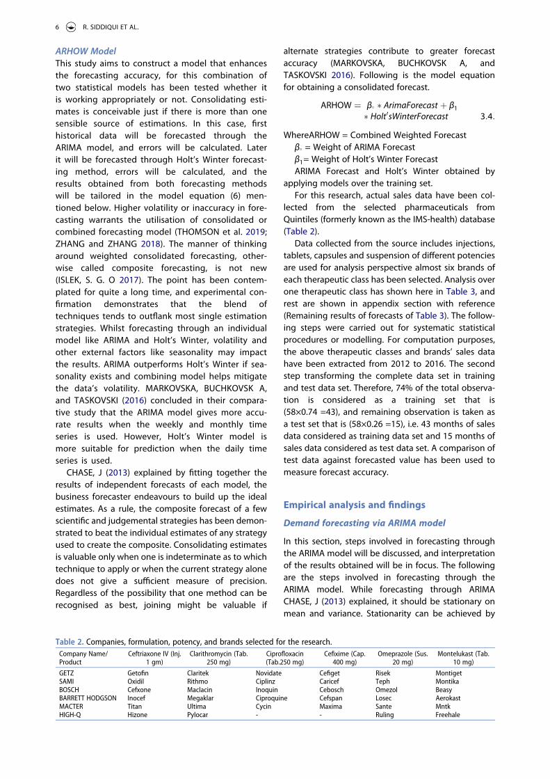
lected from the selected pharmaceuticals from Quintiles (formerly known as the IMS-health) database (Table 2).

Data collected from the source includes injections, tablets, capsules and suspension of different potencies are used for analysis perspective almost six brands of each therapeutic class has been selected. Analysis over one therapeutic class has shown here in Table 3, and rest are shown in appendix section with reference (Remaining results of forecasts of Table 3). The follow-ing steps were carried out for systematic statistical procedures or modelling. For computation purposes, the above therapeutic classes and brands’ sales data have been extracted from 2012 to 2016. The second step transforming the complete data set in training and test data set. Therefore, 74% of the total observa-tion is considered as a training set that is (58×0.74 =43), and remaining observation is taken as a test set that is (58×0.26 =15), i.e. 43 months of sales data considered as training data set and 15 months of sales data considered as test data set. A comparison of test data against forecasted value has been used to measure forecast accuracy.

Empirical analysis and findings

Demand forecasting via ARIMA model

In this section, steps involved in forecasting through the ARIMA model will be discussed, and interpretation of the results obtained will be in focus. The following are the steps involved in forecasting through the ARIMA model. While forecasting through ARIMA CHASE, J (2013) explained, it should be stationary on mean and variance. Stationarity can be achieved by

Table 2. Companies, formulation, potency, and brands selected for the research.Company Name/ Product

Ceftriaxone IV (Inj. 1 gm)

Clarithromycin (Tab. 250 mg)

Ciprofloxacin (Tab.250 mg)

Cefixime (Cap. 400 mg)

Omeprazole (Sus. 20 mg)

Montelukast (Tab. 10 mg)

GETZ Getofin Claritek Novidate Cefiget Risek MontigetSAMI Oxidil Rithmo Ciplinz Caricef Teph MontikaBOSCH Cefxone Maclacin Inoquin Cebosch Omezol BeasyBARRETT HODGSON Inocef Megaklar Ciproquine Cefspan Losec AerokastMACTER Titan Ultima Cycin Maxima Sante MntkHIGH-Q Hizone Pylocar - - Ruling Freehale

6 R. SIDDIQUI ET AL.

taking the difference of original data or by log trans-formation. Thus, by making it a stationary trend and seasonality removes from data. So as in the case, first- order differencing removes trend, and log transforma-tion tend to remove seasonality. The rest has done by ‘auto.arima’ command in ‘R’. ARIMA forecasting through the ‘R’ package automatically fit the best model over the data set based on best AIC (Akaike Information Criteria) and BIC (Bayesian Information Criteria) value (Hyndman et al., 2020). Therefore, there is no need to reinvent the wheel to fit the model and forecast manually.

Demand forecasting via holts winter model

The Holts Winter model has already been discussed earlier in the methodology section. In this section, steps involved in forecasting through the Holts Winter model will be discussed, and interpretation of the results obtained will be in focus. COGHLAN (2015) Holts Winter model is a parameter-based demand fore-casting method, so it is necessary to assign weights to parameters, i.e., alpha, beta, and gamma. More weigh-tage, i.e. near to 1, refers that the model considered most recent observations to assign more weights to forecast for a short term with accuracy. Forecast pack-age in ‘R’ has built-in capabilities if the forecast for short-term period or forecasting less than that of train-ing set package automatically assigns more weights to recent observations. The computation has been done through ‘R’ by running the command ‘forecast.holtwin-ters’ explained and applied by DHAL and RAO (2014) and ALBALAWI and ALANZI (2015) in their papers.

Demand forecasting via combine forecast/ARHOW model

Thirty-four brands of pharmaceutical sales data that belongs to 6 therapeutic class are tested and analysed. To get a complete insight of model functioning,

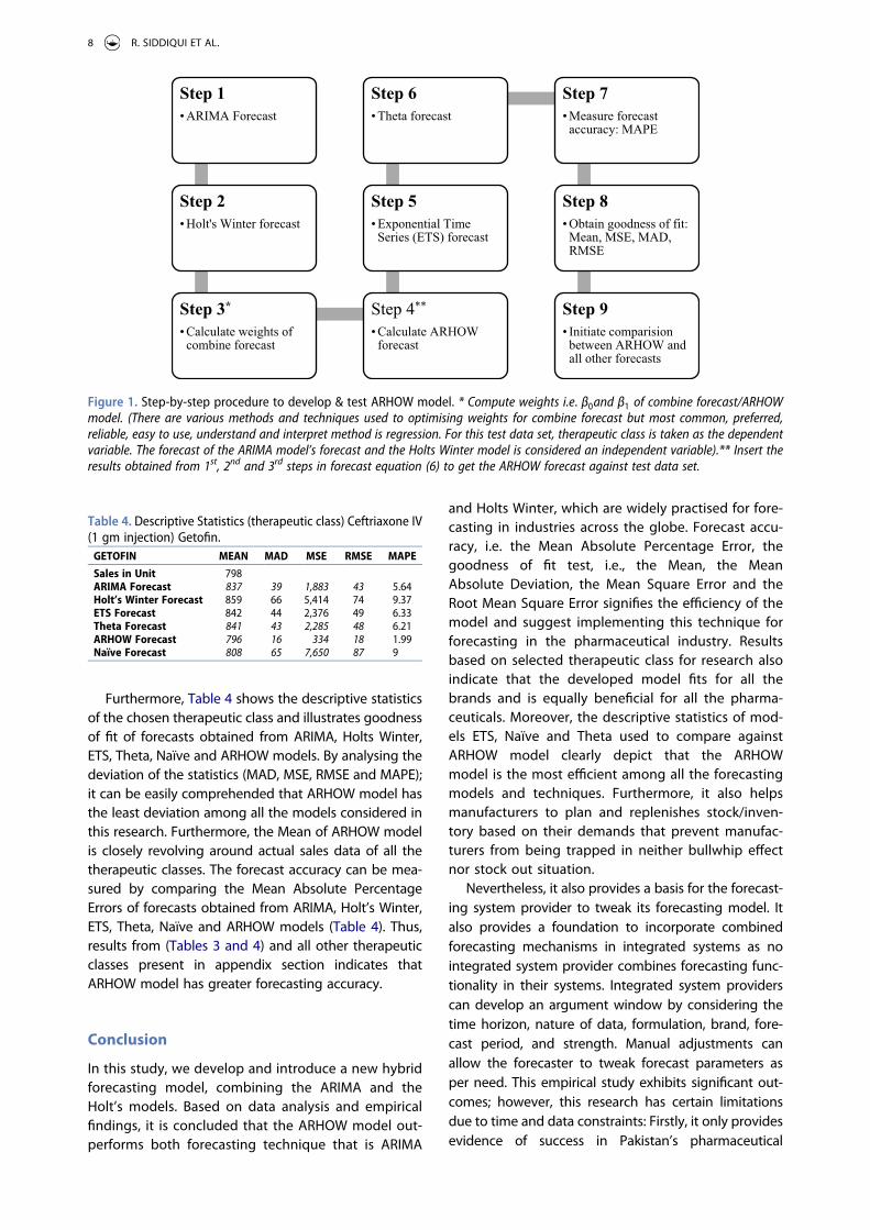
a famous brand (Getofin) of ‘Ceftriaxone’, a therapeutic class often used to cure middle ear infec-tions, meningitis, pneumonia, urinary tract infection, and other acute diseases are chosen. The method of combining the different models are not new research-ers applied this technique in their researches with slightly different/unique approaches by tweaking the combining techniques like (CAIADO 2010), (WEI and YANG 2012), (CHAN and PAUWELS 2018), (MUNIM and SCHRAMM 2020) and others applied it in many disci-plines. In this paper, the combine-forecasting techni-que has been applied in a slightly different manner. Figure 1 indicates a step-by-step procedure to test the efficiency of the model:

Results

To further test the efficiency and validity of the ARHOW model, the results of two more models; Exponential Time Series (ETS) and Theta are compared and illu-strated in Table 3. By comparing the result of ARHOW forecast against ARIMA, Holts-Winter, ETS and Theta forecast, it is concluded that the ARHOW forecast is still significantly better concerning the models used in this study.

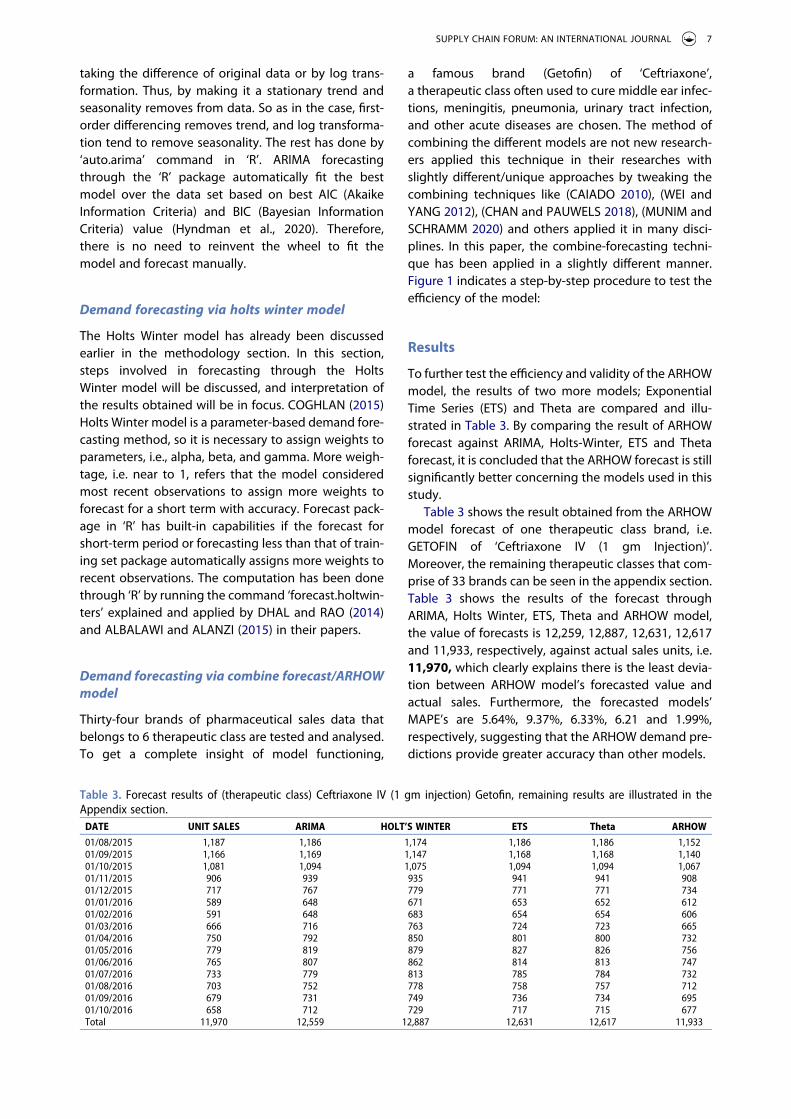
Table 3 shows the result obtained from the ARHOW model forecast of one therapeutic class brand, i.e. GETOFIN of ‘Ceftriaxone IV (1 gm Injection)’. Moreover, the remaining therapeutic classes that com-prise of 33 brands can be seen in the appendix section. Table 3 shows the results of the forecast through ARIMA, Holts Winter, ETS, Theta and ARHOW model, the value of forecasts is 12,259, 12,887, 12,631, 12,617 and 11,933, respectively, against actual sales units, i.e. 11,970, which clearly explains there is the least devia-tion between ARHOW model’s forecasted value and actual sales. Furthermore, the forecasted models’ MAPE’s are 5.64%, 9.37%, 6.33%, 6.21 and 1.99%, respectively, suggesting that the ARHOW demand pre-dictions provide greater accuracy than other models.

Table 3. Forecast results of (therapeutic class) Ceftriaxone IV (1 gm injection) Getofin, remaining results are illustrated in the Appendix section.

DATE UNIT SALES ARIMA HOLT’S WINTER ETS Theta ARHOW

01/08/2015 1,187 1,186 1,174 1,186 1,186 1,15201/09/2015 1,166 1,169 1,147 1,168 1,168 1,14001/10/2015 1,081 1,094 1,075 1,094 1,094 1,06701/11/2015 906 939 935 941 941 90801/12/2015 717 767 779 771 771 73401/01/2016 589 648 671 653 652 61201/02/2016 591 648 683 654 654 60601/03/2016 666 716 763 724 723 66501/04/2016 750 792 850 801 800 73201/05/2016 779 819 879 827 826 75601/06/2016 765 807 862 814 813 74701/07/2016 733 779 813 785 784 73201/08/2016 703 752 778 758 757 71201/09/2016 679 731 749 736 734 69501/10/2016 658 712 729 717 715 677Total 11,970 12,559 12,887 12,631 12,617 11,933

SUPPLY CHAIN FORUM: AN INTERNATIONAL JOURNAL 7

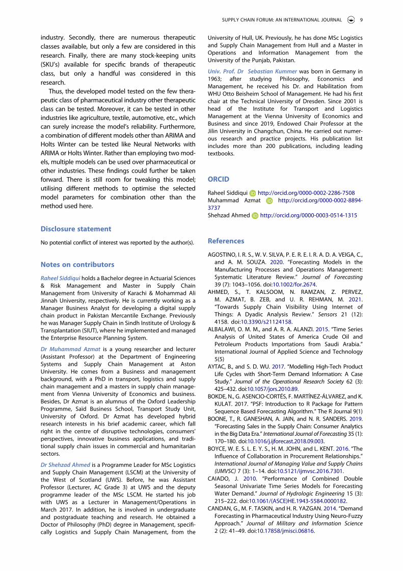
Furthermore, Table 4 shows the descriptive statistics of the chosen therapeutic class and illustrates goodness of fit of forecasts obtained from ARIMA, Holts Winter, ETS, Theta, Naïve and ARHOW models. By analysing the deviation of the statistics (MAD, MSE, RMSE and MAPE); it can be easily comprehended that ARHOW model has the least deviation among all the models considered in this research. Furthermore, the Mean of ARHOW model is closely revolving around actual sales data of all the therapeutic classes. The forecast accuracy can be mea-sured by comparing the Mean Absolute Percentage Errors of forecasts obtained from ARIMA, Holt’s Winter, ETS, Theta, Naïve and ARHOW models (Table 4). Thus, results from (Tables 3 and 4) and all other therapeutic classes present in appendix section indicates that ARHOW model has greater forecasting accuracy.

Conclusion

In this study, we develop and introduce a new hybrid forecasting model, combining the ARIMA and the Holt’s models. Based on data analysis and empirical findings, it is concluded that the ARHOW model out-performs both forecasting technique that is ARIMA

and Holts Winter, which are widely practised for fore-casting in industries across the globe. Forecast accu-racy, i.e. the Mean Absolute Percentage Error, the goodness of fit test, i.e., the Mean, the Mean Absolute Deviation, the Mean Square Error and the Root Mean Square Error signifies the efficiency of the model and suggest implementing this technique for forecasting in the pharmaceutical industry. Results based on selected therapeutic class for research also indicate that the developed model fits for all the brands and is equally beneficial for all the pharma-ceuticals. Moreover, the descriptive statistics of mod-els ETS, Naïve and Theta used to compare against ARHOW model clearly depict that the ARHOW model is the most efficient among all the forecasting models and techniques. Furthermore, it also helps manufacturers to plan and replenishes stock/inven-tory based on their demands that prevent manufac-turers from being trapped in neither bullwhip effect nor stock out situation.

Nevertheless, it also provides a basis for the forecast-ing system provider to tweak its forecasting model. It also provides a foundation to incorporate combined forecasting mechanisms in integrated systems as no integrated system provider combines forecasting func-tionality in their systems. Integrated system providers can develop an argument window by considering the time horizon, nature of data, formulation, brand, fore-cast period, and strength. Manual adjustments can allow the forecaster to tweak forecast parameters as per need. This empirical study exhibits significant out-comes; however, this research has certain limitations due to time and data constraints: Firstly, it only provides evidence of success in Pakistan’s pharmaceutical

Step 1• ARIMA Forecast

Step 2• Holt's Winter forecast

Step 3*

• Calculate weights of combine forecast

Step 4**

• Calculate ARHOW forecast

Step 5• Exponential Time Series (ETS) forecast

Step 6• Theta forecast

Step 7 • Measure forecast

accuracy: MAPE

Step 8• Obtain goodness of fit:

Mean, MSE, MAD, RMSE

Step 9• Initiate comparision

between ARHOW and all other forecasts

Figure 1. Step-by-step procedure to develop & test ARHOW model. * Compute weights i.e. β0and β1 of combine forecast/ARHOW model. (There are various methods and techniques used to optimising weights for combine forecast but most common, preferred, reliable, easy to use, understand and interpret method is regression. For this test data set, therapeutic class is taken as the dependent variable. The forecast of the ARIMA model’s forecast and the Holts Winter model is considered an independent variable).** Insert the results obtained from 1st, 2nd and 3rd steps in forecast equation (6) to get the ARHOW forecast against test data set.

Table 4. Descriptive Statistics (therapeutic class) Ceftriaxone IV (1 gm injection) Getofin.

GETOFIN MEAN MAD MSE RMSE MAPE

Sales in Unit 798ARIMA Forecast 837 39 1,883 43 5.64Holt’s Winter Forecast 859 66 5,414 74 9.37ETS Forecast 842 44 2,376 49 6.33Theta Forecast 841 43 2,285 48 6.21ARHOW Forecast 796 16 334 18 1.99Naïve Forecast 808 65 7,650 87 9

8 R. SIDDIQUI ET AL.

industry. Secondly, there are numerous therapeutic classes available, but only a few are considered in this research. Finally, there are many stock-keeping units (SKU’s) available for specific brands of therapeutic class, but only a handful was considered in this research.

Thus, the developed model tested on the few thera-peutic class of pharmaceutical industry other therapeutic class can be tested. Moreover, it can be tested in other industries like agriculture, textile, automotive, etc., which can surely increase the model’s reliability. Furthermore, a combination of different models other than ARIMA and Holts Winter can be tested like Neural Networks with ARIMA or Holts Winter. Rather than employing two mod-els, multiple models can be used over pharmaceutical or other industries. These findings could further be taken forward. There is still room for tweaking this model; utilising different methods to optimise the selected model parameters for combination other than the method used here.

Disclosure statement

No potential conflict of interest was reported by the author(s).

Notes on contributors

Raheel Siddiqui holds a Bachelor degree in Actuarial Sciences & Risk Management and Master in Supply Chain Management from University of Karachi & Mohammad Ali Jinnah University, respectively. He is currently working as a Manager Business Analyst for developing a digital supply chain product in Pakistan Mercantile Exchange. Previously he was Manager Supply Chain in Sindh Institute of Urology & Transplantation (SIUT), where he implemented and managed the Enterprise Resource Planning System.

Dr Muhammad Azmat is a young researcher and lecturer (Assistant Professor) at the Department of Engineering Systems and Supply Chain Management at Aston University. He comes from a Business and management background, with a PhD in transport, logistics and supply chain management and a masters in supply chain manage-ment from Vienna University of Economics and business. Besides, Dr Azmat is an alumnus of the Oxford Leadership Programme, Saïd Business School, Transport Study Unit, University of Oxford. Dr Azmat has developed hybrid research interests in his brief academic career, which fall right in the centre of disruptive technologies, consumers' perspectives, innovative business applications, and tradi-tional supply chain issues in commercial and humanitarian sectors.

Dr Shehzad Ahmed is a Programme Leader for MSc Logistics and Supply Chain Management (LSCM) at the University of the West of Scotland (UWS). Before, he was Assistant Professor (Lecturer, AC Grade 3) at UWS and the deputy programme leader of the MSc LSCM. He started his job with UWS as a Lecturer in Management/Operations in March 2017. In addition, he is involved in undergraduate and postgraduate teaching and research. He obtained a Doctor of Philosophy (PhD) degree in Management, specifi-cally Logistics and Supply Chain Management, from the

University of Hull, UK. Previously, he has done MSc Logistics and Supply Chain Management from Hull and a Master in Operations and Information Management from the University of the Punjab, Pakistan.

Univ. Prof. Dr Sebastian Kummer was born in Germany in 1963; after studying Philosophy, Economics and Management, he received his Dr. and Habilitation from WHU Otto Beisheim School of Management. He had his first chair at the Technical University of Dresden. Since 2001 is head of the Institute for Transport and Logistics Management at the Vienna University of Economics and Business and since 2019, Endowed Chair Professor at the Jilin University in Changchun, China. He carried out numer-ous research and practice projects. His publication list includes more than 200 publications, including leading textbooks.

ORCID

Raheel Siddiqui http://orcid.org/0000-0002-2286-7508Muhammad Azmat http://orcid.org/0000-0002-8894- 3737Shehzad Ahmed http://orcid.org/0000-0003-0514-1315

References

AGOSTINO, I. R. S., W. V. SILVA, P. E. R. E. I. R. A. D. A. VEIGA, C., and A. M. SOUZA. 2020. “Forecasting Models in the Manufacturing Processes and Operations Management: Systematic Literature Review.” Journal of Forecasting 39 (7): 1043–1056. doi:10.1002/for.2674.

AHMED, S., T. KALSOOM, N. RAMZAN, Z. PERVEZ, M. AZMAT, B. ZEB, and U. R. REHMAN, M. 2021. “Towards Supply Chain Visibility Using Internet of Things: A Dyadic Analysis Review.” Sensors 21 (12): 4158. doi:10.3390/s21124158.

ALBALAWI, O. M. M., and A. R. A. ALANZI. 2015. “Time Series Analysis of United States of America Crude Oil and Petroleum Products Importations from Saudi Arabia.” International Journal of Applied Science and Technology 5(5)

AYTAC, B., and S. D. WU. 2017. “Modelling High-Tech Product Life Cycles with Short-Term Demand Information: A Case Study.” Journal of the Operational Research Society 62 (3): 425–432. doi:10.1057/jors.2010.89.

BOKDE, N., G. ASENCIO-CORTÉS, F. MARTÍNEZ-ÁLVAREZ, and K. KULAT. 2017. “PSF: Introduction to R Package for Pattern Sequence Based Forecasting Algorithm.” The R Journal 9(1)

BOONE, T., R. GANESHAN, A. JAIN, and N. R. SANDERS. 2019. “Forecasting Sales in the Supply Chain: Consumer Analytics in the Big Data Era.” International Journal of Forecasting 35 (1): 170–180. doi:10.1016/j.ijforecast.2018.09.003.

BOYCE, W. E. S. L. E. Y. S., H. M. JOHN, and L. KENT. 2016. “The Influence of Collaboration in Procurement Relationships.” International Journal of Managing Value and Supply Chains (IJMVSC) 7 (3): 1–14. doi:10.5121/ijmvsc.2016.7301.

CAIADO, J. 2010. “Performance of Combined Double Seasonal Univariate Time Series Models for Forecasting Water Demand.” Journal of Hydrologic Engineering 15 (3): 215–222. doi:10.1061/(ASCE)HE.1943-5584.0000182.

CANDAN, G., M. F. TASKIN, and H. R. YAZGAN. 2014. “Demand Forecasting in Pharmaceutical Industry Using Neuro-Fuzzy Approach.” Journal of Military and Information Science 2 (2): 41–49. doi:10.17858/jmisci.06816.

SUPPLY CHAIN FORUM: AN INTERNATIONAL JOURNAL 9

CHAN, F., and L. L. PAUWELS. 2018. “Some Theoretical Results on Forecast Combinations.” International Journal of Forecasting 34 (1): 64–74. doi:10.1016/j.ijforecast.2017.08.005.

CHASE, J, C. H. A. R. L. E. S. W. 2013. Demand-Driven Forecasting, New Jersey, USA. John Wiley & Sons, .

COGHLAN, A. 2015. “A Little Book of R for Time Series.” In A Little Book of R for Time Series.

DEY, A. N, D. E. B. A. S. H. R. I. 2013. “Study on Key Issues and Critical Success Factors of E-Supply Chain Management in Health Care Services.” International Journal of Advanced Computer Research 3: 7–13.

DHAL, R. R., and B. P. RAO. 2014. “Shrinking The Uncertainty In Online Sales Prediction With Time Series Analysis.” ICTACT Journal on Soft Computing 2(1)

DHAMO, E., and L. PUKA “Using the R-Package to Forecast Time Series: ARIMA Models and Application”. International Conference Economic & Social Challenges And Problems, Oslo, Norway, 2010.

Dufour, Jean-Marie, and Julien Neves. “Finite-sample infer-ence and nonstandard asymptotics with Monte Carlo tests and R.” In Handbook of Statistics, vol. 41, pp. 3–31. Elsevier, 2019

DURAND, T. 2003. “Twelve Lessons from ‘Key Technologies 2005ʹ: The French Technology Foresight Exercise.” Journal of Forecasting 22 (2–3): 161–177. doi:10.1002/for.856.

EPICOR. 2017. “Improve Operations And Profitability With A Solution Built For Manufacturers” [Online]. US: EPICOR. Available: http://www.epicor.com/manufacturing/manu facturing-software.aspx [Accessed]

ERKAYMAN, B. 2018. “Transition to A JIT Production System through ERP Implementation: A Case from the Automotive Industry.” International Journal of Production Research 57 (17): 5467–5477. doi:10.1080/ 00207543.2018.1527048.

CRONE, and F. D. S. 2013. “Forecasting with SAP APO DP” [Online]. Lancaster, UK: av. Available: https://www.lancas ter.ac.uk/media/lancaster-university/content-assets/docu ments/lums/fo recasting/LCFSAPAPO-DP(coursebro chure).pdf [Accessed 01-03-20172017].

FILDES, R., and P. GOODWIN. 2020. “Stability in the Inefficient Use of Forecasting Systems: A Case Study in A Supply Chain Company.” International Journal of Forecasting 16(1)

FILDES, R., P. GOODWIN, and D. ÖNKAL. 2019. “Use and Misuse of Information in Supply Chain Forecasting of Promotion Effects.” International Journal of Forecasting 35 (1): 144–156. doi:10.1016/j.ijforecast.2017.12.006.

FORDYCE, K. 2009. “The Ongoing Challenge – Improving Organizational Performance with Better Decisions. SIAM Conference on “Mathematics for Industry”.” Society for Industrial and Applied Mathematics (SIAM) 19–30.

GALARRAGA, O., M. E. O’BRIEN, J. P. GUTIERREZ, F. RENAUD- THERY, B. D. NGUIMFACK, M. BEUSENBERG, K. WALDMAN, A. SONI, S. M. BERTOZZI, and R. GREENER. 2007. “Forecast of Demand for Antiretroviral Drugs in Low and Middle- Income Countries: 2007–2008.” AIDS 21 (4): S97–103. doi:10.1097/01.aids.0000279712.32051.29.

GELPER, S., R. FRIED, and C. CROUX. 2010. “Robust Forecasting with Exponential and Holt–Winters Smoothing.” Journal of Forecasting 29: 285–300.

GÉRARD, P. C., and A. L. MARTIN. 2001. “Contracting to Assure Supply: How to Share Demand Forecasts in a Supply Chain.” Informs 47: 629–646.

Gujarati, D.N., Porter, D.C. and Gunasekar, S., 2012. Basic econometrics. Tata McGraw-Hill Education

GUPTA, A., and D. M. COSTAS. 2000. “A Two-Stage Modeling and Solution Framework for Multisite Midterm Planning under Demand Uncertainty.” Industrial & Engineering Chemistry Research 39 (10): 3799–3813. doi:10.1021/ ie9909284.

HASIN, M. A. A., S. GHOSH, and M. A. SHAREEF. 2011. “An ANN Approach to Demand Forecasting in Retail Trade in Bangladesh.” International Journal of Trade, Economics and Finance 2: 154–160. doi:10.7763/IJTEF.2011.V2.95.

HININGS, B., T. GEGENHUBER, and R. GREENWOOD. 2018. “Digital Innovation and Transformation: An Institutional Perspective.” Information and Organization 28 (1): 52–61. doi:10.1016/j.infoandorg.2018.02.004.

Hyndman, Rob J., and Yeasmin Khandakar. “Automatic time series forecasting: the forecast package for R.” Journal of statistical software 27, no. 1 (2008): 1–22

IM, G., A. RAI, and L. S. LAMBERT. 2019. “Governance and Resource-Sharing Ambidexterity for Generating Relationship Benefits in Supply Chain Collaborations.” Decision Sciences 50 (4): 656–693. doi:10.1111/deci.12353.

INFOR. 2017. “Documentation Infor Center” [Online]. Available: https://docs.infor.com/help_m3kpd_15.1.2/ index.jsp?topic=%2Fcom.lawson.help.scplanhs-uwa% 2Fcfc0500.html [Accessed]

ISLEK, S. G. O, I. R. E. M. “A Decision Support System for Demand Forecasting Based on Classifier Ensemble.” 2017 Istanbul. Communication papers of the Federated Conference on Computer Science and Information Systems, Prague. 35–41.

JHARKHARIA, S., and R. SHANKAR. 2005. “IT-enablement of Supply Chains: Understanding the Barriers.” Journal of Enterprise Information Management 18 (1): 11–27. doi:10.1108/17410390510571466.

JR., C. W. C. 2013. Demand-Driven Forecasting: A Structured Approach to Forecasting, Hoboken. NewJersy, USA: Wiley Online Library.

KIELY, D. 2004. “The State of Pharmaceutical Industry Supply Planning and Demand Forecasting.” Journal of Business Forecasting Methods & Systems 23: 20–22.

LAOUAFI, A., M. MORDJAOUI, and D. DIB “Very Short-Term Electricity Demand Forecasting Using Adaptive Exponential Smoothing Methods”. 2014 15th International Conference on Sciences and Techniques of Automatic Control and Computer Engineering (STA), 2014. Hammamet, Tunisia, IEEE, 553–557.

LI, T., and M. YU. 2017. “Coordinating a Supply Chain When Facing Strategic Consumers.” Decision Sciences 48 (2): 336–355. doi:10.1111/deci.12224.

MARKOVSKA, M., A. BUCHKOVSK A, and D. TASKOVSKI. 2016. Comparative Study of ARIMA and Holt-Winters Statistical Models for Prediction of Energy Consumption. Macedonia. Research Gate.

Merkuryeva, G., Valberga, A. and Smirnov, A., 2019. Demand forecasting in pharmaceutical supply chains: A case study. Procedia Computer Science, 149, pp.3–10

Moritz, S., Sardá, A., Bartz-Beielstein, T., Zaefferer, M. and Stork, J., 2015. Comparison of different methods for uni-variate time series imputation in R. arXiv preprint arXiv:1510.03924

MUNIM, Z. H., and H.-J. SCHRAMM. 2017. “Forecasting Container Shipping Freight Rates for the Far East – Northern Europe Trade Lane.” Maritime Economics & Logistics 19 (1): 106–125. doi:10.1057/s41278-016-0051-7.

MUNIM, Z. H., and H.-J. SCHRAMM. 2020. “Forecasting Container Freight Rates for Major Trade Routes: A Comparison of Artificial Neural Networks and Conventional Models.” In Maritime Economics & Logistics, 1–18.

10 R. SIDDIQUI ET AL.

NASIRI, M., J. UKKO, M. SAUNILA, and T. RANTALA. 2020. “Managing the Digital Supply Chain: The Role of Smart Technologies.” Technovation 96-97: 102121. doi:10.1016/j. technovation.2020.102121.

NIKOLOPOULOS, K., S. BUXTON, M. KHAMMASH, and P. STERN. 2016. “Forecasting Branded and Generic Pharmaceuticals.” International Journal of Forecasting 32 (2): 344–357. doi:10.1016/j.ijforecast.2015.08.001.

ORACLE. 2017. “JD Edwards EnterpriseOne Applications Forecast Management Implementation Guide” [Online]. US: ORACLE Help Center. Available: https://docs.oracle. com/cd/E16582_01/doc.91/e15111/und_forecast_levels_ methods.htm#EOAFM00165 [Accessed]

PAPAGEORGIOU, L. G. 1931-1938 (2009). “Supply Chain Optimisation for the Process Industries: Advances and Opportunities.” In: MARIANTHI IERAPETRITOU, M. B. A. E. P., Ed. International Conference on Foundations of Computer-Aided Process Operations. Torrington Place. Science Direct.

PETERSEN, H. 2004. “Integrating The Forecasting Process With The Supply Chain: Bayer Healthcare’s Journey.” Journal of Business Forecasting Methods & Systems 22: 11–16.

PHILLIPS, C. J., and K. NIKOLOPOULOS. 2019. “Forecast Quality Improvement with Action Research: A Success Story at PharmaCo.” International Journal of Forecasting 35 (1): 129–143. doi:10.1016/j. ijforecast.2018.02.005.

PISHVAEE, M. I. R. S. A. M. A. N., and M. F. FARIBORZ JOLAI. 2008. “A Fuzzy Clustering-Based Method for Scenario Analysis in Strategic.” South African Journal of Business Management 39 (3): 21–31. doi:10.4102/ sajbm.v39i3.564.

PWC. 2016. “Pharma 2020: Supplying the Future Which Path Will You Take?” [Online]. UK: PWC Available: https://www. pwc.ch/en/publications/2016/pharma-2020-supplying- the-future.pdf [Accessed].

QAD. 2016. Forecast Simulation. Enterprise Edition 2011. USA. ed.

RADHAKRISHNAN, A., D. DAVID, D. HALES, and V. S. SRIDHARAN. 2011. “Mapping the Critical Links between Supply Chain Evaluation System and Supply Chain Integration Sustainability.” International Journal of Strategic Decision Sciences 2 (1): 44–65. doi:10.4018/ jsds.2011010103.

REES, H. 2011. Supply Chain Management in the Drug Industry: Delivering Patient Value for Pharmaceuticals and Biologics, Hoboken. NJ, USA: John Wiley & Sons, .

RUSCA, F., E. U. G. E. N. ROSCA, M. U. H. A. M. M. A. D. AZMAT, H. E. R. I. B. E. R. T. O. PEREZ-ACEBO, A. U. R. A. RUSCA, and S. E. R. G. I. U. OLTEANU “Modelling the Transit of Containers through Quay Buffer Storage Zone in Maritime Terminals”. International Scientific Conference The Science and Development of Transport (ZIRP 2020), 2020 NA. ZIRP2020. Croatia.

SAGE. 2013. “Better Inventory Management” [Online]. California: Sage. Available: http://www.forecastpro.com/ products/overview/method.htm [Accessed].

SAHAY, B. S., and R. MOHAN. 2003. “Supply Chain Management Practices in Indian Industry.” International Journal of Physical Distribution & Logistics Management 33 (7): 582–606. doi:10.1108/ 09600030310499277.

SALAM, M. A., and S. A. KHAN. 2018. “Achieving Supply Chain Excellence Through Supplier Management.” Benchmarking: An International Journal 25 (9): 4084–4102. doi:10.1108/BIJ-02-2018-0042.

SAP. 2017. “SAP Library Document Classification” [Online]. Available: http://help.sap.com/saphelp_scm700_ehp03/ helpdata/en/ab/2dc95360267614e10000000a174cb4/con tent.htm [Accessed]

SCHNIEDERJANS, D. G., C. CURADO, and M. KHALAJHEDAYATI. 2020. “Supply Chain Digitisation Trends: An Integration of Knowledge Management.” International Journal of Production Economics 220: 107439. doi:10.1016/j.ijpe.2019.07.012.

SECGINLI, S., S. ERDOGAN, and K. A. MONSEN. 2014. “Attitudes of Health Professionals Towards Electronic Health Records in Primary Health Care Settings: A Questionnaire Survey.” Informatics for Health and Social Care 39 (1): 15–32. doi:10.3109/17538157.2013.834342.

SEKHRI, N. 2006. Forecasting for Global Health: New Money, New Products & New Markets. Washington DC: Center For Global Development.

STADTLER, H., and C. KILGER. 2005. Supply Chain Management And Advanced Planning. Berlin, Germany: Springer, Berlin, Heidelberg.

THOMSON, M. E., A. C. POLLOCK, D. ÖNKAL, and M. S. GÖNÜL. 2019. “Combining Forecasts: Performance and Coherence.” International Journal of Forecasting 35 (2): 474–484. doi:10.1016/j.ijforecast.2018.10.006.

Tiwari, S., 2020. Supply chain integration and Industry 4.0: a systematic literature review. Benchmarking: An International Journal(28)

Tomasgard, A. and Høeg, E., 2005. A supply chain optimiza-tion model for the Norwegian Meat Cooperative. In Applications of stochastic programming (pp. 253–276). Society for Industrial and Applied Mathematics

WALTERS, D., and N. P. ARCHER. 2006. “Demand Chain Effectiveness – Supply Chain Efficiencies.” Journal of Enterprise Information Management 19 (3): 246–261. doi:10.1108/17410390610658441.

WEI, X., and Y. YANG. 2012. “Robust Forecast Combinations.” Journal of Econometrics 166 (2): 224–236. doi:10.1016/j. jeconom.2011.09.035.

WELLER, M., and D. S. CRONE. 2012. “Supply Chain Forecasting: Best Practices & Benchmarking Study.” Lancaster Centre For Forecasting 1: 1–43.

Whewell, R., 2016. Supply chain in the pharmaceutical indus-try: strategic influences and supply chain responses. CRC Press

WHO. 2016. Global Demand Forecasts for HIV Diagnostics in Low- and Middle-Income Countries from 2015 to 2020. GENEVA: UNAIDS.

YURDAL, D. I. A. C. O. N. U. R. C., and MEHMET 2017. Microsoft Web Page. Online Microsoft Website. Available: https:// www.microsoft.com/en-us/download/confirmation.aspx? id=43128

ZERAATI, H., L. RAJABION, H. MOLAVI, and N. J. NAVIMIPOUR. 2019. “A Model for Examining the Effect of Knowledge Sharing and New IT-Based Technologies on the Success of the Supply Chain Management Systems.” Kybernetes 49 (2): 229–251. doi:10.1108/K-06-2018-0280.

ZHANG, Y.-J., and J.-L. ZHANG. 2018. “Volatility Forecasting of Crude Oil Market: A New Hybrid Method.” Journal of Forecasting 37 (8): 781–789. doi:10.1002/for.2502.

SUPPLY CHAIN FORUM: AN INTERNATIONAL JOURNAL 11