a hybrid boundary for the prediction of intake wave

Title:

A HYBRID BOUNDARY FOR THE PREDICTION OF INTAKE WAVE DYNAMICSIN I.C. ENGINES

Authors:

M.F. Harrison*1 and R. Perez Arenas1,2

*corresponding author

Professional addresses:

1 School of Engineering,Cranfield University, Cranfield, Bedfordshire MK43 0AL, England

2 Now at Ricardo MTC LtdSoutham Road, Radford Semele, Leamington Spa, Warwickshire CV31 1FQ, England

Correspondence to:

Dr Matthew HarrisonSchool of Engineering

Whittle BuildingCranfield University

CranfieldBedfordshire MK43 0AL

Reference: HYBRID BOUNDARY, Revision 1 (19th November 2002)

Total number of pages of text: 35 (including this page)Total number of figures: 226851 words

lb01lzq

Text Box

Journal of Sound and Vibration, Volume 270, Issues 1-2, 6 February 2004, Pages 111-136.

M.F. Harrison, R. Perez Arenas HYBRID BOUNDARY, Revision 1

2

Abstract

This paper concerns the calculation of wave dynamics in the intake systems of naturally

aspirated internal combustion (I.C.) engines. In particular it presents a method for improving

the boundary conditions required to solve the one-dimensional Euler equations that are

commonly used to describe the wave dynamics in time and space.

A number of conclusions are reached in this work. The first relates to the quasi-steady state

inflow boundary specified in terms of ingoing and outgoing characteristics that is commonly

adopted for engine simulation. This is correctly specified by using the pair of primitive

variables pressure (p) and density (ρ) but will be unrealistic at frequencies above a Hemholtz

number of 0.1 as only stagnation values po, ρo are used. For the case of I.C. engine intake

simulations this sets a maximum frequency of around 300Hz. Above that frequency the

results obtained will become increasingly unrealistic.

Secondly, a hybrid time and frequency domain boundary has been developed and tested

against linear acoustic theory. This agrees well with results obtained using a quasi-steady

state boundary at low frequencies (Helmholtz number less than 0.1) and should remain

realistic at higher frequencies in the range of Helmholtz number 0.1 - 1.84.

Thirdly, the cyclic nature of the operation of the IC engine has been exploited to make use of

the inverse Fourier transform to develop an analytical hybrid boundary that functions for non-

sinusoidal waves in ducts. The method is self starting, does not rely on iterations over

complete cycles and is entirely analytical and therefore is an improvement over earlier hybrid

boundaries.


3

1 Introduction

Intense sound waves are formed in the intake systems of I.C. (internal combustion) engines.

A proportion of the sound power contained in these waves is radiated as intake orifice noise

and is of primary interest to vehicle refinement engineers. Poor control of intake orifice noise

may result in the failure of the legislative pass by noise test or may cause adverse comment

from potential customers.

The sound waves can also affect the power performance of naturally aspirated I.C. engines

[1]. By phasing the waves so that a high pressure is caused directly behind the intake valve

20-50o of crankshaft rotation before it closes, the volumetric efficiency of the engine can be

improved. At low volumetric efficiencies, the sound waves are the resonant response of the

intake system to excitation caused by unsteady mass flow through the intake valve [2]. At

higher volumetric efficiencies, for instance those found in racing engines, the conversion of

inflow momentum to static pressure rise on the back of the closing inlet valves is also

important [3].

This paper concerns the calculation of the wave dynamics in the intake systems of naturally

aspirated I.C. engines. In particular it presents a method for improving the boundary

conditions required to solve the one-dimensional Euler equations that are commonly used to

describe the wave dynamics in time and space.

Section 2 opens with a discussion of possible boundary conditions to solve the Euler

equations in one dimension. It goes on to explain why quasi steady state boundary conditions


4

expressed in the form of Riemann invariants are almost exclusively used in the time domain

simulation of engine performance. The limitations of such boundaries are considered.

Section 3 describes a hybrid boundary that uses the results of a linear acoustic model to

generate a frequency variable (and therefore non-quasi steady state) boundary that may be

expressed in terms of Riemann invariants.

Section 4 compares the results of calculations made using a traditional quasi steady state

boundary condition with the results obtained using the hybrid boundary. Conclusions are

drawn in Section 5.

2 Boundary conditions to the 1-D Euler equations

The general equations that govern fluid motion can easily be written down if the scalar and

vector conservation laws are applied to an arbitrary control volume [4]. These can be

reduced to the Euler equations by setting the viscosity and the thermal conductivity

coefficient to zero. By considering one-dimensional flow only, the Euler equations are the

following continuity, momentum and energy equations:

0xu

ρxρ

utρ

(1)

efxp

ρ1

xu

utu

(2)


5

0fuq1γρxρ

utρ

axp

utp

e2

(3)

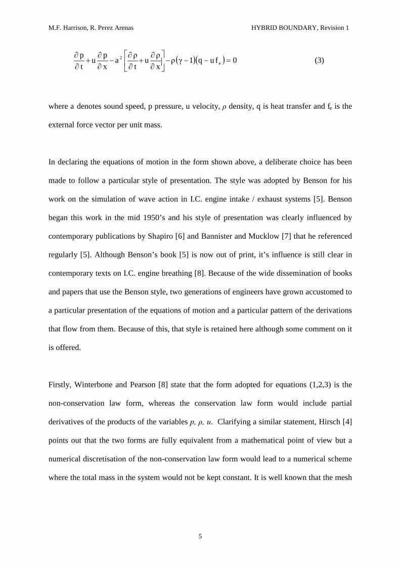
where a denotes sound speed, p pressure, u velocity, ρ density, q is heat transfer and fe is the

external force vector per unit mass.

In declaring the equations of motion in the form shown above, a deliberate choice has been

made to follow a particular style of presentation. The style was adopted by Benson for his

work on the simulation of wave action in I.C. engine intake / exhaust systems [5]. Benson

began this work in the mid 1950’s and his style of presentation was clearly influenced by

contemporary publications by Shapiro [6] and Bannister and Mucklow [7] that he referenced

regularly [5]. Although Benson’s book [5] is now out of print, it’s influence is still clear in

contemporary texts on I.C. engine breathing [8]. Because of the wide dissemination of books

and papers that use the Benson style, two generations of engineers have grown accustomed to

a particular presentation of the equations of motion and a particular pattern of the derivations

that flow from them. Because of this, that style is retained here although some comment on it

is offered.

Firstly, Winterbone and Pearson [8] state that the form adopted for equations (1,2,3) is the

non-conservation law form, whereas the conservation law form would include partial

derivatives of the products of the variables p, ρ, u. Clarifying a similar statement, Hirsch [4]

points out that the two forms are fully equivalent from a mathematical point of view but a

numerical discretisation of the non-conservation law form would lead to a numerical scheme

where the total mass in the system would not be kept constant. It is well known that the mesh


6

method of characteristics which is based on a discretisation of the non-conservation law form

does not conserve mass.

Secondly, equations (2,3) differ a little from those shown in [5,8] wherein the friction term fe

is replaced by

D4

fuu21

G (4)

where D is the hydraulic diameter of the duct and f is the wall friction factor. Bannister and

Mucklow included such a term in their calculation scheme [7]. The modulus of the velocity is

introduced to ensure that the pipe wall friction always opposes the fluid motion. In the

equations of motion presented here, G is replaced by an external force vector per unit mass fe.

This avoids the use of equation (4), which is a specific friction model that relies on empirical

data for f and the assumption that the friction increases with the square of the velocity. This

argument is rather an academic one, as fe is eventually neglected in the analysis in Section 2.1

on the assumption of a thin boundary, but the presence of fe rather than G in equations (2,3)

warrants a brief explanation.

The equations of motion (1,2,3) together form a set of three simultaneous partial differential

equations with three independent variables p, ρ and u, with a linked variable a where

ργp

a 2 (5)

The equations need both initial and boundary conditions for their solution.


7

The initial conditions simply require the definition of the spatial distribution of the primitive

flow variables ρ, u, p along with the appropriate thermodynamic data; temperature (T), the

gas constant (R), the specific heat capacities (cp, cv) and the heat transfer q.

Boundary conditions require more detailed consideration which follows in Section 2.1.

2.1 Boundary conditions: primitive variables and characteristic variables

Stationary solid boundaries should only reflect waves travelling out from the interior of the

control volume. They should not emit or absorb waves. However, so-called far-field

boundaries should allow waves to travel in and out of the control volume [10]. Far-field

boundary conditions must allow an outgoing wave to pass without reflection and in turn

specify a corresponding in-going wave.

In-going waves carry information from the exterior to the control volume. Assuming that the

boundary is thin so that the thermodynamic quantities are the same on the inner and outer

surfaces, that information could take the form of:

(i) Conserved quantities (mass, momentum, energy)

(ii) Primitive flow variables (ρ, u, p)

(iii) So called characteristic variables (vo, v+, v-)

The characteristic variables will be derived from equations (1,2,3) in the pattern set out by

Benson [5] for the same reason that the form of the equations of motion (1,2,3) was adopted.


8

However, the interested reader might seek alternative patterns. For example, Landau and

Lifshitz [9] derive the two characteristic variables required for the analysis of homentropic

flow in only a few lines of text.

The derivation of the characteristic variables is as follows.

The continuity equation (1) and the momentum equation (2) and the energy equation (3) can

be linearly combined to give two characteristic equations [8]:

0fρafuq1γρxu

autu

aρxp

autp

ee

(6)

0fρafuq1γρxu

autu

aρxp

autp

ee

(7)

The energy equation (3) provides a third characteristic equation [8].

By defining three characteristic lines where:

autdxd

(8)

a-utdxd (9)

utdxd (10)


9

the three partial differential characteristic equations (6,7,3) can be transformed into three

ordinary differential equations known as compatibility relationships (11,12,13):

0faρfuq1γρtdud

aρtdpd

ee (11)

for the case when autdxd

0fρafuq1γρtdud

aρtdpd

ee (12)

for the case when autdxd

0faρfuq1γρtdρd

atdpd

ee2 (13)

for the case when utdxd

For the case of a thin boundary q and fe are set to zero. Inflow to a practical intake pipe is a

fairly homentropic process. Thus, we can assume ds = 0 across the boundary where s denotes

specific entropy. The three homentropic compatibility relationships can be extracted from

(11,12,13) thus:

autdxd

for0tdud

aρtdpd

(14)

autdxd

for0tdud

aρtdpd

(15)


10

utdxd

for0tdρd

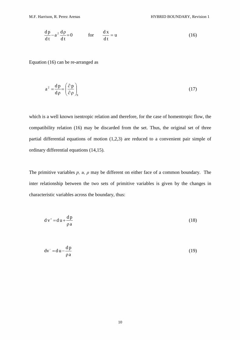
atdpd 2 (16)

Equation (16) can be re-arranged as

S

2

ρp

ρdpd

a

(17)

which is a well known isentropic relation and therefore, for the case of homentropic flow, the

compatibility relation (16) may be discarded from the set. Thus, the original set of three

partial differential equations of motion (1,2,3) are reduced to a convenient pair simple of

ordinary differential equations (14,15).

The primitive variables p, u, ρ may be different on either face of a common boundary. The

inter relationship between the two sets of primitive variables is given by the changes in

characteristic variables across the boundary, thus:

aρpd

udvd (18)

aρpd

uddv (19)


11

2.2 The inflow boundary: Riemann invariants

The ultimate boundary for the I.C. engine intake system is that of subsonic inflow to a pipe.

In this case it can be shown that two quantities only are required to properly specify the

boundary [10].

The boundary is properly specified if the exterior information given uniquely determines the

incoming characteristic variables when combined with interior information, but these do not

restrict or specify the outgoing characteristic variable.

Specifying only one exterior primitive variable for the subsonic inflow case obviously under

specifies the problem. Specifying all three primitive exterior variables would specify the

outgoing characteristic value as well as the ingoing characteristic values and therefore the

boundary would be incorrect.

Therefore, two exterior primitive variables should be specified. These may be ρ and p or

equally ρ and u but not u and p because the last case would completely specify both ingoing

and outgoing characteristic variables [10], (see equations 18,19).

To summarise, ingoing and outgoing characteristic values must be considered as a set if a

boundary is to be considered to be valid.

From the second law of thermodynamics, and assuming an isentropic process we get

dp = da1γ

a2ρ

(20)


12

Substituting (20) into (18) and (19) and integrating along the characteristic lines we get the

Riemann invariants:

u2

1γavλ

λ constant when au

tdxd

(21)

u2

1γavβ

β constant when au

tdxd

(22)

For the general boundary case we could specify:

(i) Ingoing conserved mass and momentum

(ii) Ingoing p and ρ or ρ and u (and s if non-homentropic)

(iii) Ingoing β if λ is the outgoing Riemann invariant (a modified and non-invariant λ is

used if the flow is non-homentropic [5])

For the inflow boundary case it would be difficult to specify the conserved quantities as these

cannot be measured directly. The pair of measurable primitive variables ρ, u could be

specified but some method of estimating both ρ and u would be required.

It would seem obvious to specify the pair of primitive variables p and ρ for the inflow

boundary. The former of these quantities is easily measured. However, it is only practical to

specify the exterior quantities in terms of their static steady state values po and ρo. To do

otherwise would require either a separate analytical model for time varying p and ρ or an


13

exterior computational grid bounded by a half space. Specifying the static values for p and ρ

involves the making of several implicit assumptions. Firstly the boundary is (quasi) steady

state. Secondly the amplitude of sound radiated from the inflow orifice is negligibly small

compared with the static pressure.

Both of the above assumptions are tolerable for application to the intake of a low speed I.C.

engine where the intake wave action is dominated by frequency components of pressure

below 100Hz [2, 11] but would be less appropriate for high speed engines where wave action

occurs at 500Hz or more [3].

Most of the widely used computer codes for I.C. engine simulation use an inflow boundary

that specifies po and ρo. However, they generally express these in terms of characteristic

variables (Riemann invariants mostly) so as to describe the boundary in terms of outgoing

and ingoing waves that are easily understood. European examples of this include: Benson’s

mesh method of characteristics [5], Winterbone and Pearsons total variation diminishing flux

limiter method [8, 12], Giannatta’s essentially non-oscillatory finite volume method [13, 14]

and Onorati’s Lax Wendroff and Mac Cormack method [15]. All four use Riemann variables

to formulate their inflow boundary. The derivation of this common boundary is as follows.

We start with:

ρpγ

a 2 (23)

This presents the primitive pair p, ρ in terms of one variable sound speed a.


14

From (21) (22)

2βλ

a

(24)

1γβλ

u

(25)

The non-conservative momentum equation down a streamline in isentropic flow (Fanno flow)

can be written [16]:

222o u

21γ

aa

(26)

where γ is the ratio of specific heat capacities.

Substituting (24) and (25) into (26) gives on re-arrangement [5]:

21

2

2

2o λ

1γγ3

1a1γ1γ

4λ1γγ3

aβ

(27)

Equation (27) is used to define the system inflow boundary in a number of IC engine

simulations [12-15] even though the numerical schemes employed to solve the equations of

fluid motion differ in each case. The implications of the use of equation (27) are this. Firstly,

equation (27) expresses the incoming Riemann invariant β in terms of the fluctuating

outgoing Riemann invariant λ, the (fluctuating) gas temperature and chemistry that govern γ,


15

and the stagnation speed of sound. With the inclusion of that stagnation datum, the boundary

becomes quasi-steady state. Secondly, the use of equation (26) in the derivation of (27)

means that homentropic, non-viscous, non-rotational inflow is assumed with the absence of

external forces. Thus, despite the apparent complexity of equation (27) with its many

bracketed terms, it actually models a rather idealised boundary condition.

To summarise the discussion in this section of the paper: the inflow boundary may be

specified using the primitive variable pair ρo, po and inspection of the characteristic variables

shows this to be one of several correct boundary choices. Alternatively, the ratio of these two

and the isentropic assumption may be used to yield a boundary specified by stagnation sound

speed ao and the outgoing characteristic variable. This approach has been widely used to

supply an inflow boundary to very different numerical schemes for solving the 1-D Euler

equations.

3 A hybrid boundary to the 1-D Euler equations

In the previous section it was shown how ao and λ could be used to specify an inflow

boundary and, hence, determine β. Although this boundary is correctly specified (it uses only

the primitive pair p, ρ) it is not accurate at higher frequencies as it is specified by stagnation

conditions only. Thus, it is a quasi-steady-state boundary.

The solution of the 1-D Euler equations would be improved for the inflow case (and other

cases that otherwise rely on quasi-steady-state boundaries) if a dynamic boundary could be

devised. One such boundary is described here.


16

The premise for the hybrid boundary is simple. The correct ratio of fluctuation acoustic

pressure to particle velocity may be calculated from linear plane wave acoustic theory at any

given plane in a duct upstream from the point of inflow [17]. This ratio varies with frequency

and can be used as a boundary condition if λ is given and β is found from the isentropic

relation

1γγ2

o0 aa

PP

(28)

and on substitution of (24) we get

1γγ2

o0 a2βλ

PP

(29)

Knowing (29) and (25) we can write

1γβλ

Pa2βλ

P

u~p~

TT

0

1γγ2

o

T

0

(30)

λT and βT are time retarded values of the characteristic variables at the hybrid boundary. This

time shifting is an important part of the hybridisation and will be discussed later. Equation

(30) has been solved iteratively [18] although an analytical solution can be found, thus:

Let TTT

u1γβλ

(31)


17

ζu~p~ (32)

Equation (30) becomes:

o

1γγ2

o

T

oT p

a2βλ

puζ

γ21γ

o

oT

o

T

ppuζ

a2βλ

Tγ21γ

o

oT

o λp

puζa2β

(33)

Unlike the quasi-steady state boundary described by equation (27), equation (33) describes a

dynamic boundary where time varying primitive variables p, u are used as input along with

ao, ,λ and γ.

If the outgoing Riemann variable λ is a strict sinusoid then a single value of ζ is calculated

from linear acoustic theory and either equation (30) is solved iteratively or equation (33) is

solved directly. If λ is not sinusoidal then ζ(f) must be transposed to the time domain using

the inverse Fourier transform before equations (30) and (33) can be used.

The present hybrid boundary has certain advantages over some alternative hybrid boundaries

that are also based on the Riemann variables. Payri et al [19] used a modified method of


18

characteristics to solve the 1-D Euler equations. This produced time domain values for

positive and negative going pressure waves, which could be transformed to the frequency

domain using the fast Fourier transform. These pressure components could then be combined

with the output from a linear acoustic model to provide a new set of pressure components,

which became pressure time values with the application of the inverse Fourier transform.

The method was iterative, solving the hybrid boundary for one complete cycle at a time. The

results of the calculations therefore updated only once every cycle. An initial pressure and

velocity field had to be assumed for the calculation to start.

Harrison and Davies [20] developed a hybrid boundary that was analytical and did not require

updating on a cycle by cycle basis nor did it require an initial sound field to start. However,

it relied on a simplified means of estimating the value of u (t) at the hybrid boundary based

on the gradients of nearby characteristic lines.

The present hybrid boundary is an alternative to the early Harrison and Davies boundary that

neither requires an initial sound field to start nor does it require an estimate of u (t) at the

hybrid boundary. Both these attributes are seen as useful developments in the field of hybrid

boundaries.

The details of the hybrid boundary will now be presented starting with the simplest case

when λ is sinusoidal and progressing to the more general case where λ is cyclic but not

sinusoidal. In either case the first step is to calculate a time shift for the hybrid boundary.

Figure 1 shows the general test case where a length of pipe has a source at the left-hand end

and an open-end boundary at the other end. The source produces a pressure fluctuation and λ


19

characteristics propagate from left to right in this case. There is no net mass inflow at the

right-hand end. The propagation is calculated using the mesh method of characteristics

(MOC) [5].

3.1 Preliminary calculations made using a quasi-steady state boundary for the open-

end of a pipe without inflow

We declare for the moment that the open-end boundary is a quasi steady state pressure

release boundary. This is a simplification of the inflow boundary described in Section 2.2 but

is more realistic for the test case that involves a sinusoidal pressure excitation without mean

flow. The quasi steady state open-end pipe boundary may be derived from the general hybrid

boundary (33). In the open ended pipe case p = po for all time and (33) reduces to:

λp

pp2aβ

γ21γ

o

oo

0uζp T in this case

λa2β o (34)

Figure 2 shows the time history for λ at a point in the pipe that is 0.1m from the source

(hereafter called the hybrid plane), calculated with a ‘pure’ MOC and using the boundary

given by equation (34) at the right hand end of the pipe. The calculation starts with the fluid

at rest in the pipe so that:


20

oau2

1λaλ

(35)

The calculation proceeds with the source producing a 96Hz pressure sinusoid with a peak

pressure of 2Pa. Close scrutiny of Figure 2 shows that the value of λ remains at the initial

level equal to ao for a short time. That time is the time it takes for the λ ‘wave’ to propagate

from the source plane to the hybrid plane, i.e.

TIMEλ =a

0.1m ≃oa

0.1 ≃ 0.000293 seconds (36)

where a is the time average wave speed during that short interval.

The λ wave continues to propagate until it reaches the open-end boundary where it is

reflected and a β wave is created in accordance with equation (34). That β wave propagates

from right to left in this case.

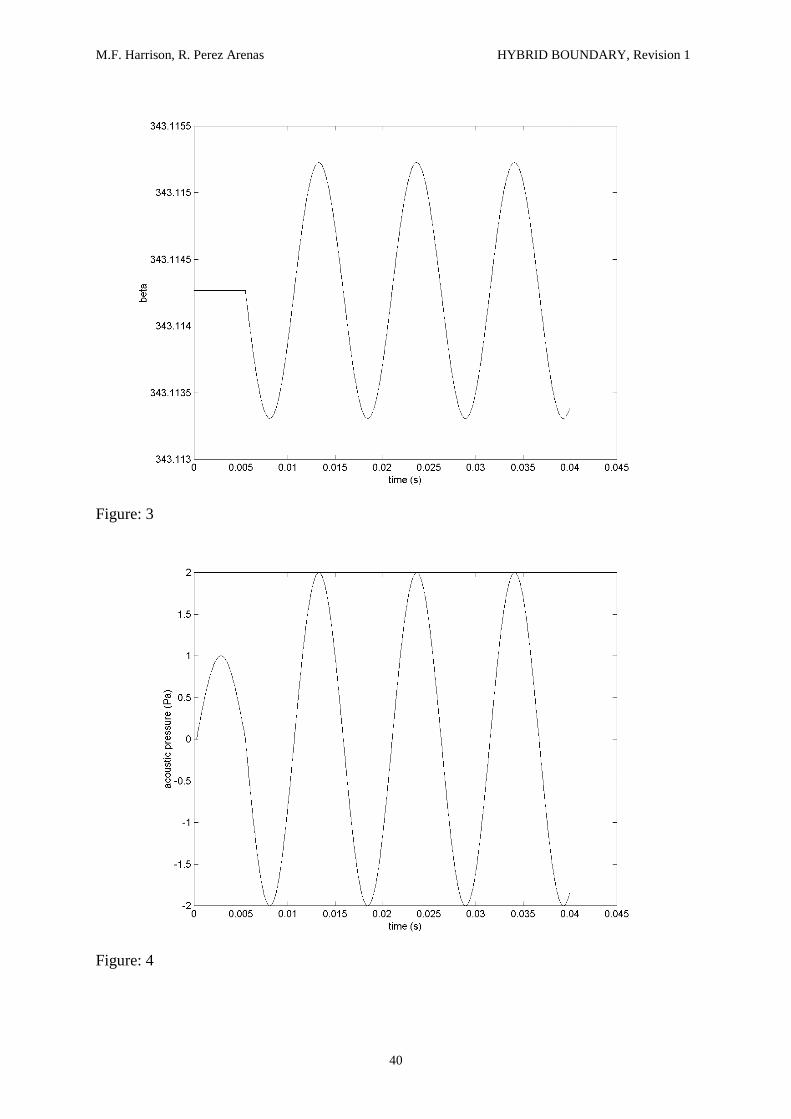
Figure 3 shows the time history of β at the hybrid plane. For the first 0.006 seconds β

remains at its initial value:

oo au2

1γaβ

(37)

This is the time it takes for the λ wave to travel from the source to the open end plus the time

taken for the β wave thus created to travel back to the hybrid plane.


21

TIMEβ ≃a

0.880.98 ≃ oa

1.86 ≃ 0.00545 seconds (38)

The implications of these two time delays λTIME and βTIME are clearly shown in Figures 4 and

5. Figure 4 shows the pressure time history at the hybrid boundary given by:

o

1γγ2

oo p

a2βλ

p'p

(39)

For the period zero seconds to λTIME, λ = β = ao and p = 0 (Figure: 2). For the time period

λTIME to βTIME λ has a fluctuating value (Figure: 2) and β = ao (Figure: 3). The fluctuating

pressure has a maximum value is 1Pa (Figure: 4). After βTIME seconds, both λ and β have

fluctuating values and the fluctuating pressure has a maximum value of 2Pa clearly

demonstrating the superposition of the λ and β waves. The fluctuation frequency of 96Hz

was chosen deliberately to produce a pressure maximum at the hybrid plane.

Figure 5 shows the particle velocity at the hybrid boundary given by equation (25).

For the period λTIME , λ = β = ao and u = 0 (Figure: 2). For the time period λTIME to βTIME λ

has a fluctuating value and β = ao (Figure: 3). A fluctuating particle velocity is produced with

a maximum amplitude given by (Figure: 5):

MAXu ≃oo

MAX

aρp ≃

343.11x1.191 ≃ 2.4 x 10-3 ms-1 (40)


22

After the period βTIME, λ ≃ β and u ≃ 0 (Figure: 5). A near zero particle velocity is expected

at the hybrid plane when a maximum fluctuating pressure is encountered as shown in

Figure 4.

Figure 5 highlights one of the problems associated with the mesh method of characteristics,

that is a spurious velocity transient formed early in the calculation when the calculation is

started from conditions of rest in the pipe. That transient will propagate up and down the

pipe and will take many cycles to decay [21]. The problem may be avoided if the calculation

starts with the non-stagnation conditions in the duct being specified by some other

(simplified) model [20] such as the one given in [2, 3].

3.2 Calculations made using a hybrid boundary for the case of an the open-ended

pipe without inflow

We return to the general test case in Figure 1. We declare a hybrid boundary (30 or 33) at the

hybrid plane. For that hybrid boundary to work correctly when used with the mesh method

of characteristics, the λ and β time histories at the hybrid plane should match those produced

from the pure method of characteristics (Figures 2, 3). This can be achieved when the

following rules are observed:

(i) For the time period t = 0 to t = βTIME, β at the hybrid plane must retain its initial value.


23

(ii) Thereafter, β may be calculated using either (30 or 33) providing that at time t, the

value of λ used is that corresponding to λ (t – δt) = λT

δt = βTIME – λTIME (41)

and the value of u used is the one corresponding to u (t – δt) = uT.

When the sound in the pipe is purely sinusoidal, ζ (f) may be calculated at that frequency

only and equation (30 or 33) may be solved in a time marching mesh method of

characteristics calculation providing the time shift rules above are observed. In this case ζ (f)

has been found using the theory developed by Davies [17] which has been applied with

success to the intake systems of practical I.C. engines [2, 3]. Figures 6 and 7 show the λ and

β time histories respectively for a hybrid calculation solving equation (30) for the case of a

2Pa pressure fluctuating pressure at 96Hz. The 2Pa at 96Hz problem was used earlier in

Section 3.1 for a pure method of characteristics calculation with a quasi steady state boundary

at the open end. The fact that the results in Figures 2 and 6 and Figures 3 and 7 match closely

is validation that the hybrid method is working correctly. Close inspection of the four figures

show that although the two sets of λ values agree perfectly the two sets of β values do not.

The λ values are determined solely by the source, which is identified for both calculations so

the two sets of λ values should match perfectly. The two sets of β values match perfectly

once the hybrid values have converged. The requirement for convergence is due to the use of

uT in equation (40), where uT requires updated values of both λT and β before it is correct.

The imperfect yet close match between the two sets of β values occurred because the sound

wave is at a low frequency (96Hz).


24

At low frequencies (Helmholtz number < 0.1) the acoustic reflection coefficient at the open

unflanged end of the pipe is almost unity [17]. The quasi-steady state open end boundary

(equation 34) used for the pure mesh method of characteristics calculations reported in

Section 3.1 implicitly states that the reflection coefficient is unity. In this case the duct

simulated had a diameter of 38mm (Figure: 1) so the Helmholtz number is 0.033 at 96Hz. At

higher frequencies, say above 300Hz where the Helmholtz number is above 0.1 and the

acoustic reflection coefficient at the open end becomes significantly less than unity [17], the

two sets of β values would differ from each other. Assuming that the hybrid results for β

remain correct at high frequencies then those produced using a quasi steady state open-end

boundary are only correct below about 300Hz for typical intake duct diameters. 300Hz

corresponds to only 1.5 times the firing frequency of a 4-cylidner engine running at 6000

rev/min-1. As the intake pressure waveform is known to contain components at 3 or more

times the firing frequency [2, 11] it seems that the realism of the quasi steady state open-end

boundary is reduced at higher engine speeds. It has been found however that the quasi-steady

state open boundary can give acceptable results, providing that a frequency varying end

correction is added to the physical pipe length [21, 22]. This is possible when the calculation

involves a sinusoidal waveform but impossible for the general case because no single end

correction would be correct for every frequency component in a (as yet un-converged and

hence unknown) non-sinusoidal sound wave.

This problem may solved by using an extension to the hybrid method discussed so far.

Equations (30 or 33) are still used along with the time shifting rules but rather than use one

value of ζ (f) as when λ is sinusoidal, the inverse Fourier transform (IFFT) of ζ (f) is used

when λ is non-sinusoidal.


25

ζ (f) should be calculated at a binary number of frequencies. The binary number n should be

large enough so that:

so ffn (42)

where fo is the lowest cycle frequency (i.e. the 4-stroke cycle frequency or the lowest

frequency input by the source in Figure 1) and:

xΔa

f os ≃

MAXtΔ1

(43)

where ∆tMAX is an approximation to the maximum time step allowed in a mesh method of

characteristics with a mesh size ∆x. The correct maximum step size is given by:

uaxΔ

Δt

(44)

ζ (f) is calculated using linear acoustic theory for the frequency range 0Hz to fs/2 Hz at

intervals given by fs/n. For the case of a 10mm mesh size and a cycle frequency of 50Hz, n =

1024. This means that calculations are being made at frequencies up to fs/2 = 28.16kHz.

This is obviously well above the plane wave cutoff frequency given by a Helmholtz number

equal to 1.84 and therefore higher mode waves will be propagating that are not included in

the linear acoustic theory employed to calculate ζ (f) [17]. The need to include spurious high

frequency results for ζ (f) is an unavoidable limitation of the method. The effects are


26

minimised if the reflection coefficient at the open end is made to tend to zero at higher

frequencies.

For a 4-stroke I.C. engine at 6000 rev/min, fo = 50Hz. The n + 1 frequency points describing

ξ(f) are then transformed into n time points for ξ(t) by the action of the IFFT.

The time marching method of characteristics calculation is performed withofn

1Δt . In this

way, n time points are used to calculate one full cycle at the lowest known cycle frequency fo.

As the IFFT provides n values for ζ (t), each value in turn can be used in solving equation

(30) or (33) for the first and any subsequent cycles. Thus ζ (t) is only calculated once but it

may be used several times if more than one cycle is simulated. In the case of an IC engine

intake system, a new ζ (t) must be calculated if the engine speed is changed (fo changes) or if

the engine load changes (the mean inlet Mach number changes and hence ξ(f) changes [17]).

4 Results

The general test case shown in Figure 1 will be used to test:

(i) The mesh method of characteristics using a quasi-steady state open-end boundary

(given by equation (34)).

(ii) The hybrid method using the mesh method of characteristics coupled with a hybrid

boundary that is the solution to equation (30) with a sinusoidal λ wave.


27

(iii) As for (ii) but solving equation (30) iteratively with a non-sinusoidal λ wave.

(iv) As for (iii) but solving equation (33) directly.

In each case, results at the hybrid plane will be reported for a 2Pa input at the source

maintained over a 0.045 second period. These will be compared with the results of the linear

acoustic theory [17], which is known to validate well against experiment for such a case [23,

24].

Figure 8 shows how the acoustic pressure ratio calculated at the hybrid plane using linear

acoustic theory varies with frequency. The acoustic pressure ratio is given by the ratio of

positive-going and negative-going travelling wave components:

p

ppwhere p+ = 1 (45)

At resonance, the modulus of the pressure ratio is maximum (96Hz) and it is minimum at

anti-resonance (192Hz).

Figure 9 shows the corresponding acoustic particle velocity given by:

oo aρpp

u

(46)

This time the modulus of the acoustic particle velocity is a minimum at resonance and a

maximum at anti-resonance.


28

Figure 10 shows the spectrum of specific acoustic impedance ratio ζ (f) given by:

pp

R(47)R1R1

ζ (48)

Peaks in the modulus of ζ (f) correspond to resonances and minima occur at anti-resonances.

For each of the four time domain calculation schemes considered here to be realistic, the

results for acoustic pressure ratio, acoustic particle velocity and specific acoustic impedance

ratio should all agree with the results obtained from linear acoustic theory.

Figure 11, 12 and 13 show the results from the pure mesh method of characteristics with the

quasi steady state boundary given by equation (34). This time acoustic pressure ratio is given

by:

MAXo

o

pppp

(49)

and the maximum value of the modulus of p from the last cycle calculated is taken. The

other two results are given by (25) and (32). All these results agree closely with linear

acoustic theory although there are some differences around the anti-resonance frequencies.

Figure 14, 15 and 16 show the corresponding results obtained using equation (30) to solve the

hybrid boundary with a sinusoidal λ wave. Again the pressure ratio and particle velocity

results agree well, but the specific acoustic impedance ratio obtained is rather low this time.

The final value obtained at resonance is found to be very sensitive to the frequency resolution


29

applied at the source: small changes in the input frequency move the starred point near 96Hz

quite significantly.

Figures 17, 18 and 19 show the results obtained by solving equation (30) iteratively with non-

sinusoidal λ waves. The pressure ratio results (Figure 17) agree closely with linear acoustic

theory but the particle velocity results less so (Figure 18). The agreement is found to depend

on the spectral resolution of ζ (f) and the corresponding number of time points in ζ (t). The

agreement between specific acoustic impedance ratio results remains acceptable though.

Figures 20, 21 and 22 show the results of solving equation (33) directly with non-sinusoidal

waves. These results agree completely with those obtained from the solution to equation (30)

as they should.

5 Conclusions

A number of conclusions have been reached in this work.

Firstly, the quasi-steady state inflow boundary specified in terms of ingoing and outgoing

characteristics that is commonly adopted for engine simulation is correctly specified by using

the primitive pair p, ρ but will be unrealistic at frequencies above a Hemholtz number of

around 0.1 as only stagnation values po, ρo are used. For the case of I.C. engine intake

simulations this sets a maximum frequency of around 300Hz. Above that frequency the

results obtained will become increasingly unrealistic.


30

Secondly, a hybrid time and frequency domain boundary has been developed and tested

against linear acoustic theory. This agrees well with results obtained using a quasi-steady

state boundary at low frequencies (Helmholtz number less than 0.1), and should remain

realistic at higher frequencies in the range of Helmholtz number 0.1 - 1.84.

Thirdly, the cyclic nature of the operation of the IC engine has been exploited to make use of

the inverse Fourier transform to develop an analytical hybrid boundary that functions for non-

sinusoidal waves in ducts. The method is self starting and does not rely on iterations over

complete cycles and is entirely analytical and therefore is an improvement over earlier hybrid

boundaries.

Acknowledgements

The first author gratefully acknowledges the support of EPSRC for this work made possible

under grant No: GR/R04324.


31

References

1 A. Ohata, Y. Ishida, 1982

SAE Paper No. 820407

“Dynamic inlet pressure and volumetric efficiency of four-cycle four-cylinder

engines”

2 M. F. Harrison, P. T. Stanev, 2002

Journal of Sound and Vibration (provisionally accepted)

“A linear acoustic model for intake wave dynamics in IC engines”

3 M. F. Harrison, A. Dunkley, 2002

Journal of Sound and Vibration (in refereeing)

“The acoustics of racing engine intake systems”

4 C. Hirsch, 1988

John Wiley & Sons, New York

“Numerical computation of internal and external flows: Volume 1 – fundamentals of

numerical discretization”

5 R. S. Benson, 1982

Clarendon Press, Oxford

“The thermodynamics and gas dynamics of internal combustion engines – Volume 1”


32

6 A.H. Shapiro, 1954,

The Ronald Press

“The dynamics and thermodynamics of compressible fluid flow – Vol II”

7 F.K. Bannister, G.F. Mucklow, 1948,

Proc. I.Mech.E., 159, 269-300 (including discussion of the paper)

“Wave action following sudden release of compressed gas from a cylinder”

8 D. E. Winterbone, R. J. Pearson, 2000

Professional Engineering Publishing Ltd

“Theory of engine manifold design: wave action methods for IC engines”

9 L.D. Landau, E.M. Lifshitz, 1959,

Pergamon Press

“Fluid mechanics”

10 C. B. Laney, 1998

Cambridge University Press

“Computational gas-dynamics”

11 M. F. Harrison, P. T. Stanev, 2002

Journal of Sound and Vibration (provisionally accepted)

“Measuring wave dynamics in IC engine intake systems”


33

12 R. J. Pearson, D.E Winterbone 1996

IMechE C499/012/96

“Calculation of one-dimensional unsteady flow in internal combustion engines – how

long should it take?

13 P. Giammatta, Ordone A, 1991

IMechE C430/055/91

“Applications of a high resolution shock-capturing scheme to the unsteady flow

computation in engine ducts”

14 Anon, 2000

AVL List GmbH

“Boost users guide – Version 3.3”

15 A. Onorati, 1996

IMechE C499/052/96

“A white noise approach for rapid gas dynamic modelling of IC engine silencers”

16 P. A. Thompson, 1988

Rensselaer Polytechnic Institute

“Compressible fluid dynamics”

17 P. O. A. L. Davies, 1988

Journal of Sound and Vibration, 124(1), pp91-115

“Practical flow duct acoustics”


34

18 R. Perez Arenas, 2001

MSc Thesis, Cranfield University

“Intake orifice noise prediction: the development of a hybrid boundary”

19 F. Payri, J.M. Desantes, A.J. Torregrosa, 1995,

Journal of Sound and Vibration, 188(1), 85-110,

“Acoustic boundary condition for unsteady one-dimensional flow calculations”

20 M. F. Harrison, P. O. A. L. Davies, 1994

IMechE C487/019

“Rapid predictions of vehicle intake/exhaust radiated noise”

21 A Onorati, 1994

Journal of Sound and Vibration, 171(3), pp369-395

“Prediction of the acoustical performances of muffling pipe systems by the method of

characteristics”

22 D. E. Winterbone, M. Yoshitomi, 1990

SAE Paper No 900677

“The accuracy of calculating wave action in engine intake manifolds”


35

23 I. De Soto Boedo, 2001


“The acoustics of internal combustion engine manifolds”

24 P. Rubio Unzueta, 2001


“Quantifying throttle losses”


36

Figure labels

Figure: 1 The test case

Figure: 2 λ at the hybrid plane with a pure method of characteristics calculation, 96 Hz

Figure: 3 β at the hybrid plane with a pure method of characteristics calculation, 96 Hz

Figure: 4 Acoustic pressure at the hybrid plane with a pure method of characteristics

calculation, 96 Hz

Figure: 5 Acoustic particle velocity at the hybrid plane with a pure method of

characteristics calculation, 96 Hz

Figure: 6 λ at the hybrid plane with a single frequency hybrid calculation, 96 Hz

Figure: 7 β at the hybrid plane with a single frequency hybrid calculation, 96 Hz

Figure: 8 Acoustic pressure at the hybrid plane

Figure: 9 Acoustic particle velocity at the hybrid plane

Figure: 10 Specific acoustic impedance ratio at the hybrid plane


37

Figure 11 Acoustic pressure ratio at the hybrid plane with a pure method of

characteristics calculation (*) vs the results of the linear acoustic model (-.-.-)

Figure 12 Acoustic particle velocity at the hybrid plane with a pure method of


Figure: 13 Specific acoustic impedance ratio at the hybrid plane with a pure method of


Figure: 14 Acoustic pressure ratio at the hybrid plane with a single frequency hybrid

calculation (*) vs the results of the linear acoustic model (-.-.-)

Figure: 15 Acoustic particle velocity at the hybrid plane with a single frequency hybrid

calculation (*) vs the results of the linear acoustic model (-.-.-)

Figure: 16 Specific acoustic impedance ratio at the hybrid plane with a single frequency

hybrid calculation (*) vs the results of the linear acoustic model (-.-.-)

Figure: 17 Acoustic pressure ratio at the hybrid plane with a multi-frequency iteriative


Figure: 18 Acoustic particle velocity at the hybrid plane with a multi-frequency iterative



38

Figure: 19 Specific acoustic impedance ratio at the hybrid plane with a multi-frequency

iterative hybrid calculation (*) vs the results of the linear acoustic model (-.-.-)

Figure: 20 Acoustic pressure ratio at the hybrid plane with a multi-frequency analytical


Figure: 21 Acoustic particle velocity at the hybrid plane with a multi-frequency analytical


Figure: 22 Specific acoustic impedance ratio at the hybrid plane with a multi-frequency

analytical hybrid calculation (*) vs the results of the linear acoustic model

(-.-.-)


39

Harrison, Perez Arenas – Figures

Figure: 1

Figure: 2

Open termination boundary

0.88m

0.98m

Hybrid plane

Source boundary

pipe length


40

Figure: 3

Figure: 4


41

Figure: 5

Figure: 6


42

Figure: 7

Figure: 8


43

Figure: 9

Figure: 10


44

Figure 11

Figure 12


45

Figure: 13

Figure: 14


46

Figure: 15

Figure: 16


47

Figure: 17

Figure: 18


48

Figure: 19

Figure: 20


49

Figure: 21

Figure: 22

a hybrid boundary for the prediction of intake wave

Documents