contentsusers.abo.fi › htoivone › courses › robust › hsem.pdf · in these notes w e giv...
TRANSCRIPT

LECTURE NOTES
ON
ROBUST CONTROL BY STATE-SPACE METHODS
Hannu Toivonen

PREFACE
These lecture notes are based on a graduate course given at the Department of Chemical Engineer-ing at Åbo Akademi University. The aim has been to give a concise introduction to the state-spaceapproach to H1 control. Both continuous and discrete time as well as sampled-data systems aretreated. The material in these notes focuses on solution procedures, whereas design issues are notconsidered. Design aspects can for example be introduced via properly selected problems. Forthis purpose, a number of problems have been included. It is recommended that the numericalproblems be worked out using some available software package, such as Matlab's Robust ControlToolbox.

CONTENTS
0. INTRODUCTION 1
1. SIGNAL SPACES AND OPERATOR NORMS 3
1.1. The L2-induced norm of a linear system 31.2. A worst-case control problem 41.3. A robust stabilization problem 51.4. The H2-norm of a transfer function 61.5. Notes and references 9
2. THE CONTINUOUS-TIME H1 CONTROL PROBLEM 11
2.1. The state feedback H1 control problem 112.2. An H1 estimation problem 152.3. Solution of the H1 control problem 182.4. Notes and references 22
3. THE DISCRETE-TIME H1 CONTROL PROBLEM 28
3.1. Problem formulation 283.2. The stationary case: Solution via bilinear transformation 293.3. The discrete-time H1 control problem: A state-space approach 313.4. Notes and references 37
4. THE SAMPLED-DATA H1 CONTROL PROBLEM 40
5. H1-OPTIMAL LOW-ORDER AND FIXED-STRUCTURECONTROLLERS 48
6. MIXED H2/H1 CONTROL PROBLEMS 50
APPENDICES
APPENDIX A � THE STATE TRANSITION MATRIX 54APPENDIX B � ADJOINT OPERATORS 55

0. INTRODUCTION
The ability to deal with uncertainty is an essential part in feedback control. If the disturbances and theplant dynamics were completely known there would be no need to use feedback in order to achieve a speci�edplant response. It is precisely due to uncertainties that feedback is necessary. A simple example wherefeedback can be used to achieve good performance in spite of imperfect knowledge of both disturbances andplant dynamics is a PI-controller, by which good compensation against low-frequency disturbances can beobtained, requiring only a minimal knowledge of the plant and disturbances. In classical controller designmethods, plant uncertainties are taken into account by stability margins relating to amplitude and phase.
In many control problems it is well motivated to minimize a speci�ed cost function, often an integralof the squares of the di�erences of the outputs from their setpoint values. Optimal control methods havebeen developed to deal with these types of problems. An inherent limitation of classical optimal controlmethods is the fact that they do not explicitly take uncertainties into account. In optimal stochasticcontrol, uncertain disturbances are described as stochastic processes with speci�ed statistical properties,but plant uncertainties are not easily incorporated into this approach.
The need to treat with uncertainties in feedback control in a systematic manner has led to the de-velopment of a speci�c theory of robust control. Modern robust control theory addresses a number ofproblems which were beyond the scope of both classical control theory and the later developed optimal andstochastic control theories. In particular, it provides a systematic treatment of the robustness of controlsystems against plant uncertainties for both scalar and multivariable plants. The theory also comprisesthe solution of realistically formulated optimal control problems for uncertain plants.
These notes describe the main elements of state-space methods of modern robust control theory. Weare concerned with the control system shown in Fig. 0.1. Here u is the control signal, w is a disturbance, zis the controlled output, and y is the measured output. The disturbance is typically assumed to belong tosome appropriate signal set, which is chosen to characterize their properties or an associated uncertainty.It is assumed that the plant G is uncertain. Typically, the plant is characterized in the form
G = G0 +�
-
�
-
-
G
K
w z
yu
Fig. 0.1.
where G0 is a nominal plant model described by a linear, �nite-dimensional transfer function, and � isa plant uncertainty. The uncertainty may be due to a number of reasons, re�ecting the fact that thenominal model is only an approximate description of the true process. These include various modelingand approximation errors, time-dependent process dynamics, etc. In practice the plant uncertainty is ofcourse not completely unknown, and one can for example give upper bounds on its magnitude at variousfrequencies. This leads to a characterization of the plant uncertainty in terms of an appropriate set ofoperators of which it is assumed to be a member. In the scalar case it is often asumed that � a lineartransfer function whose frequency response satis�es the bound
j�(i!)j � jl(i!)jwhere l(i!) is a frequency weight which describes the maximum uncertainty at various frequencies. In themultivariable case, the equation should be modi�ed to
��(�(i!)) � jl(i!)j
1

where ��(�) denotes the maximum singular value of �.Given the nominal plant model, the set of disturbances and the plant uncertainty set, the problem is
to design the controller K in such a way that some speci�ed control performance is achieved. A minimumrequirement is that the closed-loop system should be stable for all plants in the speci�ed uncertainty set.The closed-loop system is then said to be robustly stable. For open-loop unstable plants the problem of�nding a controller such that the closed loop is robustly stable is by itself a well-motivated control problem.This is called the robust stabilization problem.
A more realistic characterization of practical control problems is to consider the disturbances as wellas plant uncertainties in the design procedure. For example, the disturbance may be described as a randomprocess, and the control objective could then be to minimize the expected stationary cost
Ez0(t)z(t):
The plant uncertainties can be taken into account in various ways. One approach is to minimize the costfunction for the nominal plant G0 subject to the condition that the closed loop is stable for all uncertainties� (optimal control with robust stability bound). An alternative is to minimize the worst value of the costwith respect to the uncertainty (optimal control with robust performance).
The solution of the problems outlined above is provided by H1 control theory. Robust stability canbe shown to be equivalent to a bound on the so-called H1-norm of a certain closed-loop transfer function.The robust stabilization problem is thus equivalent to an H1-optimal control problem. In a similar way,the optimal control problem with robustness against plant uncertainties is equivalent to a so-called mixedH2=H1 control problem.
In these notes we give an introduction to state-space methods for solving robust control problems.The material is organized as follows. Section 1 gives background material on signal spaces and operatornorms, which is needed in the later development. Sections 2 and 3 present state-space solutions to thestandard H1 problem for continuous-time and discrete-time systems, respectively. In Section 4, the H1
problem is presented for sampled-data systems. Section 5 gives a brief discussion of the important problemof designing low-order and �xed-structure controllers which achieve a speci�ed H1 performance bound.Mixed H2=H1 problems are described in Section 6.
2
1. SIGNAL SPACES AND OPERATOR NORMS
1.1. The L2-induced norm of a linear system
We consider signals which belong to the space L2[0;1) of square-integrable functions on [0;1), equippedwith the norm
kwk2 :=�Z 1
0
wT (t)w(t)dt
�1=2; w 2 L2[0;1) (1:1)
The Fourier transform w(i!) of w,
w(i!) :=
Z 1
0
w(t)e�i!tdt (1:2)
then belongs to the space L2(iR) of square-integrable functions on the imaginary axis iR, which is equippedwith the norm
kwk2 :=� 1
2�
Z 1
�1
w�(i!)w(i!)d!
�1=2; w 2 L2(iR) (1:3)
Here w�(i!) denotes the complex conjugate transpose, i.e., w�(i!) := w0(�i!). By Parseval's theorem, the
norms in (1.1) and (1.3) are equal, i.e.,kwk2 = kwk2 (1:4)
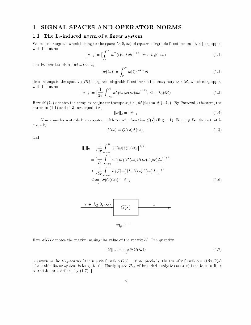
Now consider a stable linear system with transfer function G(s) (Fig. 1.1). For w 2 L2, the output isgiven by
z(i!) = G(i!)w(i!); (1:5)
and
kzk2 =� 1
2�
Z 1
�1
z�(i!)z(i!)d!
�1=2=� 1
2�
Z 1
�1
w�(i!)G�(i!)G(i!)w(i!)d!
�1=2� � 1
2�
Z 1
�1
��(G(i!))2w�(i!)w(i!)d!�1=2
� sup!
��(G(i!)) � kwk2 (1:6)
- -G(s)w 2 L2[0;1) z
Fig. 1.1.
Here ��(G) denotes the maximum singular value of the matrix G. The quantity
kGk1 := sup!
��(G(i!)) (1:7)
is known as the H1-norm of the matrix function G(�). [ More precisely, the transfer function matrix G(s)of a stable linear system belongs to the Hardy space H1 of bounded analytic (matrix) functions in Re s> 0 with norm de�ned by (1.7). ]
3
From (1.7) we see that z 2 L2 if w 2 L2 an kGk1 <1. The gain J(G) of the system is then de�nedas the L2-induced norm,
J(G) := sup
� kzk2kwk2 : w 6= 0; w 2 L2[0;1)
�= sup
� kzk2kwk2 : w 6= 0; w 2 L2(iR)
�(1:8)
Equations (1.6) and (1.7) gives an upper bound on J(G),
J(G) � kGk1In fact it can be shown that equality holds, i.e.,
J(G) = kGk1 (1:9)
[ The result can be seen to follow from (1.6) by setting the input w(i!) proportional to the singular vectorof G(i!) corresponding to the largest singular value ��(G(i!)) and concentrating all the energy of w to afrequency interval where ��(G(i!)) > sup! ��(G(i!)) � �, and forming the limit � # 0. ]
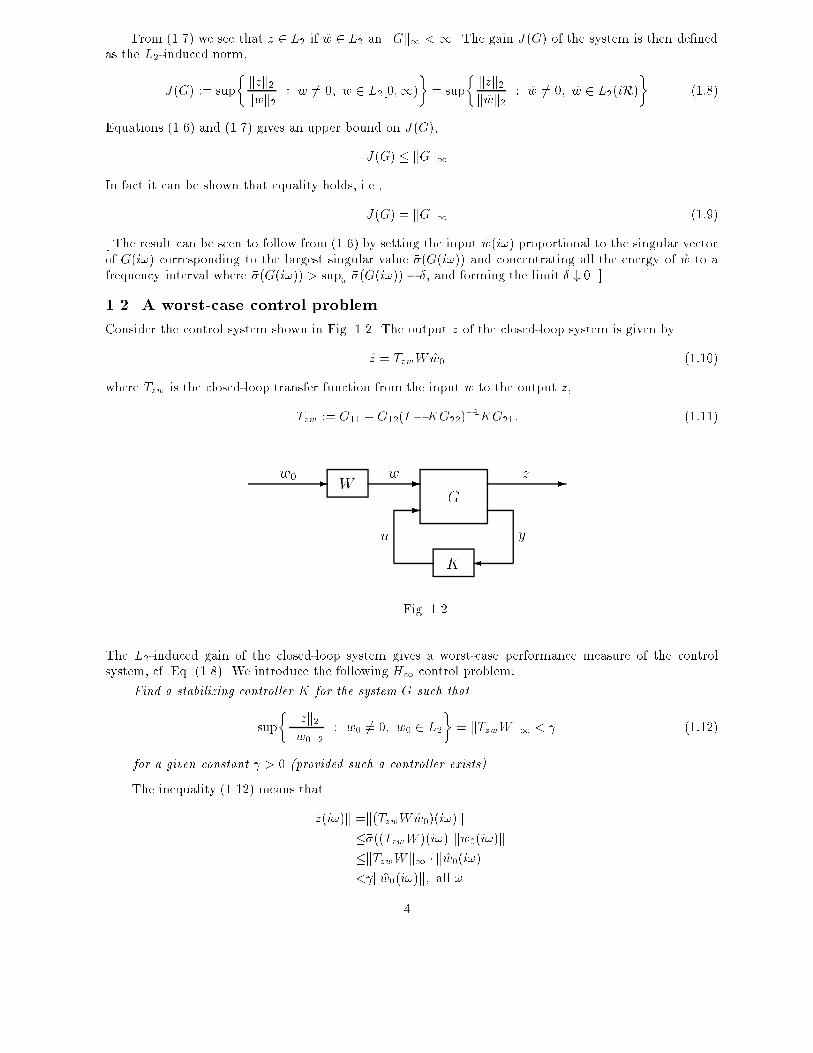
1.2. A worst-case control problem
Consider the control system shown in Fig. 1.2. The output z of the closed-loop system is given by
z = TzwWw0 (1:10)
where Tzw is the closed-loop transfer function from the input w to the output z,
Tzw := G11 + G12(I �KG22)�1KG21: (1:11)
- -
�
-
-WG
K
w0 w z
yu
Fig. 1.2.
The L2-induced gain of the closed-loop system gives a worst-case performance measure of the controlsystem, cf. Eq. (1.8). We introduce the following H1 control problem:
Find a stabilizing controller K for the system G such that
sup
� kzk2kw0k2 : w0 6= 0; w0 2 L2
�= kTzwWk1 < (1:12)
for a given constant > 0 (provided such a controller exists).
The inequality (1.12) means that
kz(i!)k =k(TzwWw0)(i!)k���((TzwW )(i!) kw0(i!)k�kTzwWk1 � kw0(i!)k< kw0(i!)k; all !
4

where k � k denotes the Euclidian norm; kzk := (z�z)1=2. Hence
kz(i!)k < kW�1(i!)w(i!)k; all !.
Hence all frequencies are attenuated uniformly with respect to the weighting �lterW (i!), which determinesthe relative importance of various frequencies.
It can be shown that the H1 control problem has the interesting property that minimizing kTzwWk1gives a closed-loop system with a constant disturbance attenuation at all frequencies:
��(Tzw(i!)W (i!)) = inf = constant
where inf := inff : kTzwWk1 < g. This is the 'equalizing property' of H1-optimal controllers. Thisproperty is useful for loop-shaping, since for a scalar weight W (i!), we have
��(Tzw(i!)) = inf=jW (i!)j;
i.e., the closed-loop frequency response of the H1-optimal controller is proportional to jW (i!)j�1.It is interesting to compare the H1-optimal control problem with the Linear Quadratic (LQ) control
problem, where the H2-norm of the closed-loop transfer function,
kTzwWk22 := tr� 1
2�
Z 1
�1
(TzwW )�(i!)(TzwW )(i!)d!�
is minimized (cf. Section 1.4 below). Here the average performance over all frequencies is considered, andthere is no guarantee that the controller attenuates all frequencies uniformly. On the other hand, theequalizing property of the H1-optimal controller implies that the H2 norm is in�nite, provided inf 6= 0.An H1-optimal controller does therefore not give good H2 performance.
1.3. A robust stabilization problem
Consider a system with additive uncertainty described by
G =
�G0 +W�A : k�A(i!)k � 1; all !
�: (1:13)
See Fig. 1.3. Here G0 is the nominal, linear time-invariant system, W is a frequency-dependent weight,and �A is a norm-bounded, but otherwise unknown uncertainty.
-?
�
-
- W�A
G0
K
i
yu
++
G
Fig. 1.3.
5
It is then of interest to study the following robust stabilization problem:
Find a controller K such that the closed-loop system in Fig. 1.3 is stable for all plants in the
set (1.13).
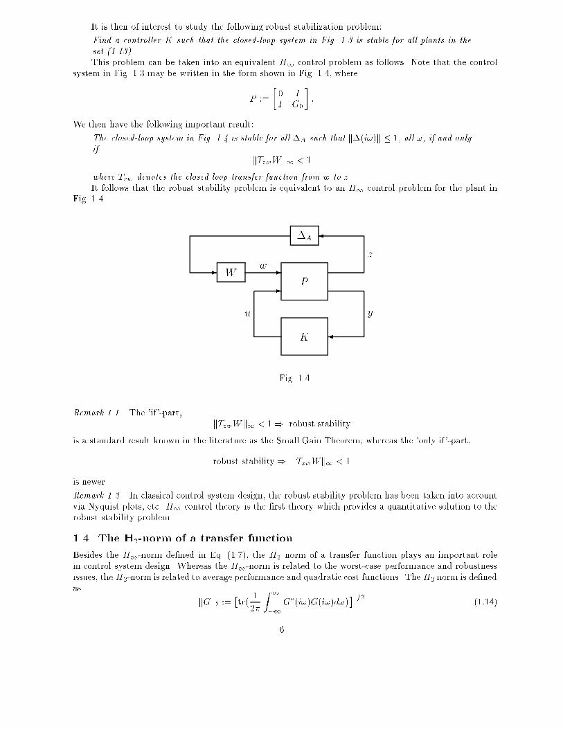
This problem can be taken into an equivalent H1 control problem as follows. Note that the controlsystem in Fig. 1.3 may be written in the form shown in Fig. 1.4, where
P :=
�0 I
I G0
�:
We then have the following important result:
The closed-loop system in Fig. 1.4 is stable for all �A such that k�(i!)k � 1, all !, if and only
if
kTzwWk1 < 1
where Tzw denotes the closed loop transfer function from w to z.
It follows that the robust stability problem is equivalent to an H1 control problem for the plant inFig. 1.4.
- -
-
�
�
�A
P
K
W
z
yu
w
Fig. 1.4.
Remark 1.1. The 'if'-part,kTzwWk1 < 1) robust stability
is a standard result known in the literature as the Small Gain Theorem, whereas the 'only if'-part,
robust stability) kTzwWk1 < 1
is newer.
Remark 1.2. In classical control system design, the robust stability problem has been taken into accountvia Nyquist plots, etc. H1 control theory is the �rst theory which provides a quantitative solution to therobust stability problem.
1.4. The H2-norm of a transfer function
Besides the H1-norm de�ned in Eq. (1.7), the H2 norm of a transfer function plays an important rolein control system design. Whereas the H1-norm is related to the worst-case performance and robustnessissues, the H2-norm is related to average performance and quadratic cost functions. The H2 norm is de�nedas
kGk2 :=�tr� 1
2�
Z 1
�1
G�(i!)G(i!)d!
��1=2(1:14)
6

The norm can also be expressed in terms of the singular values of �k(G(�)) of G(�) according to
kGk2 =� 1
2�
Xk
Z 1
�1
�2k(G(i!))d!
�1=2(1:15)
This follows from the relationtr(G�G) =
Xk
�2k(G)
An important property of the H2-norm is its relation to quadratic cost functions. Here we shall showhow a quadratic cost function for a linear stochastic system can be expressed by the H2-norm of thecorresponding transfer function. For this purpose, we introduce the linear stochastic system G describedby the state-space equation
_x = Ax+Bw
z = Cx(1:16)
Here we assume that the system is exponentially stable, i.e., the eigenvalues of A are in the open lefthalfplane. The input w is a stationary stochastic white noise process with zero mean value,
E w(t) = 0; all t (1:17a)
and the covariance functionE w(t)wT (t0) = I�(t � t
0) (1:17b)
where �(�) is the Dirac �-function, de�ned by the properties
�(s) = 0; if s 6= 0Z 1
�1
�(s)ds = 1(1:18)
Remark 1.3. Note that the case with a general covariance matrix Rw,
E w(t)wT (t0) = Rw�(t� t0)
can always be written in the form (1.16), (1.17), by de�ning B such that BB0 = Rw.
Consider the stationary quadratic cost function
J2(G) := limT!1
E[1
T
Z T
0
zTzdt] = lim
t!1E[zT (t)z(t)] (1:19)
We shall �nd explicit time-domain and frequency-domain expressions for the cost J2(G) in terms of thesystem parameters in Eq. (1.16).
Introduce the stationary covariance matrix P of the state in (1.16),
P := limT!1
E[1
T
Z T
0
x(t)xT (t)dt] = limt!1
E[x(t)xT (t)] (1:20)
Then J2(G) is given byJ2(G) = tr(CT
CP ) (1:21)
and P is given by
P =
Z 1
0
eA�BB
TeAT �
d� (1:22)
and can be obtained as the solution of the linear matrix equation (Lyapunov equation)
AP + PAT + BB
T = 0 (1:23)
7

Note here that the assumption on A, Re(�i(A)) < 0, ensures that the integral in (1.22) converges.In the frequency domain, de�ne the transfer function of the system (1.16), i.e.,
G(s) = C(sI �A)�1B (1:24)
Then J2(G) can be expressed in terms of the H2-norm of G,
J2(G) = kGk22 (1:25)
We shall present informal proofs of the above formulae. More rigorous treatments can be found in thereferences. First, (1.21) follows from
zTz = x
TCTCx = tr(CT
CxxT )
In order to show (1.22), recall that (cf. Appendix A),
x(t) =
Z t
�1
eA(t��)
Bw(� )d�
Hence
E[x(t)xT (t)] = E�Z t
�1
eA(t��)
Bw(� )d���Z t
�1
eA(t��)
Bw(�)d��T
= E�Z t
�=�1
�Z t
�=�1
eA(t��)
Bw(� )wT (�)BTeAT (t��)
d��d��
=
Z t
�=�1
�Z t
�=�1
eA(t��)
BE[w(� )wT (�)]BTeAT (t��)
d��d�
=
Z t
�1
eA(t��)
BBTeAT (t��)
d� [ by (1.17), (1.18)]
=
Z 0
�1
e�A�
BBTe�AT�
d�
=
Z 1
0
eA�BB
TeAT �
d�
= P:
To show that P is also a solution of the linear matrix equation (1.23), note that
d
d�(eA�BBT
eAT � ) =
d
d�(eA� )BBT
eAT � + e
A�BB
T d
d�(eA
T � )
= AeA�BB
TeAT � + e
A�BB
TeAT �
AT
where we have usedd
d�eA� = Ae
A� = eA�A
Hence,
AP + PAT = A
Z 1
0
eA�BB
TeAT �
d� +
Z 1
0
eA�BB
TeAT �
d�AT
=
Z 1
0
�Ae
A�BB
TeAT � + e
A�BB
TeAT �
AT�d�
=
Z 1
0
d
d�
�eA�BB
TeAT �
�d�
= eA�BB
TeAT �
����1
�=0
= �BBT
8

which shows (1.23).Finally, let's show the frequency-domain identity (1.25). By (1.21) and (1.22), we have
J2(G) = tr(CPCT )
= tr�Z 1
0
CeA�BB
TeAT �
CTd��
= trZ 1
0
H(� )HT (� )d�
where H(�) denotes the impulse response of the system (1.16),
H(� ) =
�Ce
A�B; � � 0
0; � < 0
Now, the transfer function G(s) = C(sI �A)�1B is simply the Laplace transform of the impulse responsefunction H(� ), or, the frequency response G(i!) is the Fourier transform of H(� ), since we have
Z 1
0
H(t)e�i!tdt =
Z 1
0
CeAtBe
�i!tdt
=
Z 1
0
CeAte�i!t
Bdt
=
Z 1
0
Ce�(i!I�A)t
Bdt
= C(�i!I + A)�1e�(i!I�A)tB
����1
t=0
= �C(�i!I +A)�1e�0B
= C(i!I � A)�1B
= G(i!)
The identity (1.25) then follows from the matrix equivalent of Parseval's theorem, Eq. (1.4), which saysthat the H2-norms of H(�) and G(�) are equal, i.e.,
kHk2 = kGk2
where (cf. Eqs.(1.1)�(1.4)),
kHk2 =�trZ 1
0
H(� )HT (� )d��1=2
kGk2 =�tr� 1
2�
Z 1
�1
G� (i!)G(i!)d!
��1=2
1.5. Notes and references
The H1 problem was originally introduced by Zames (1981). The solution techniques �rst developed forthe problem were based on analytic function theory and operator-theoretic methods. For an introductionto these methods, see the book by Francis (Francis 1987).
The formulation of robust stability in terms of the H1-norm (Section 1.3) is due to a number ofresearchers, see Doyle and Stein (1981), Chen and Desoer (1982), Kimura (1984), Vidyasagar (1985), andVidyasagar and Kimura (1986). Highly readable accounts of the robust stability issue are found in thebooks by Vidyasagar (1985) and McFarlane and Glover (1990).
9
PROBLEMS
1.1. Verify Parseval's theorem.
1.2. Verify the equivalence of the control systems in Figures 1.3 and 1.4.
REFERENCES
Chen, M. J., and C. A. Desoer (1982), �Necessary and Su�cient Conditions for Robust Stability of LinearDistributed Feedback Systems,� Int. J. Control 35, 255�267.
Doyle, J. C., and G. Stein (1981). �Multivariable Feedback Design: Concepts for a Classical/Modern Syn-thesis,� IEEE Trans. Automat. Control 26, 4�16.
Francis, B. (1987). A Course in H1 Control Theory, Springer-Verlag, New York.Kimura, H., (1984). �Robust Stabilizability for a Class of Transfer Functions,� IEEE Trans. Automat.
Control 29, 788�793.McFarlane, D. C., and K. Glover (1990). Robust Controller Design Using Normalized Coprime Factor Plant
Descriptions, Springer-Verlag, Berlin.Vidyasagar, M. (1985). Control System Synthesis: A Factorization Approach, MIT Press, Cambridge,
Massachusetts.Vidyasagar, M., and H. Kimura (1986). �Robust Controllers for Uncertain Linear Multivariable Systems,�
Automatica 22, 85�94.Zames, G. (1981). �Feedback and Optimal Sensitivity: Model Reference Transformations, Multiplicative
Seminorms, and Approximate Inverses,� IEEE Trans. Automat. Control 26, 301�320.
10
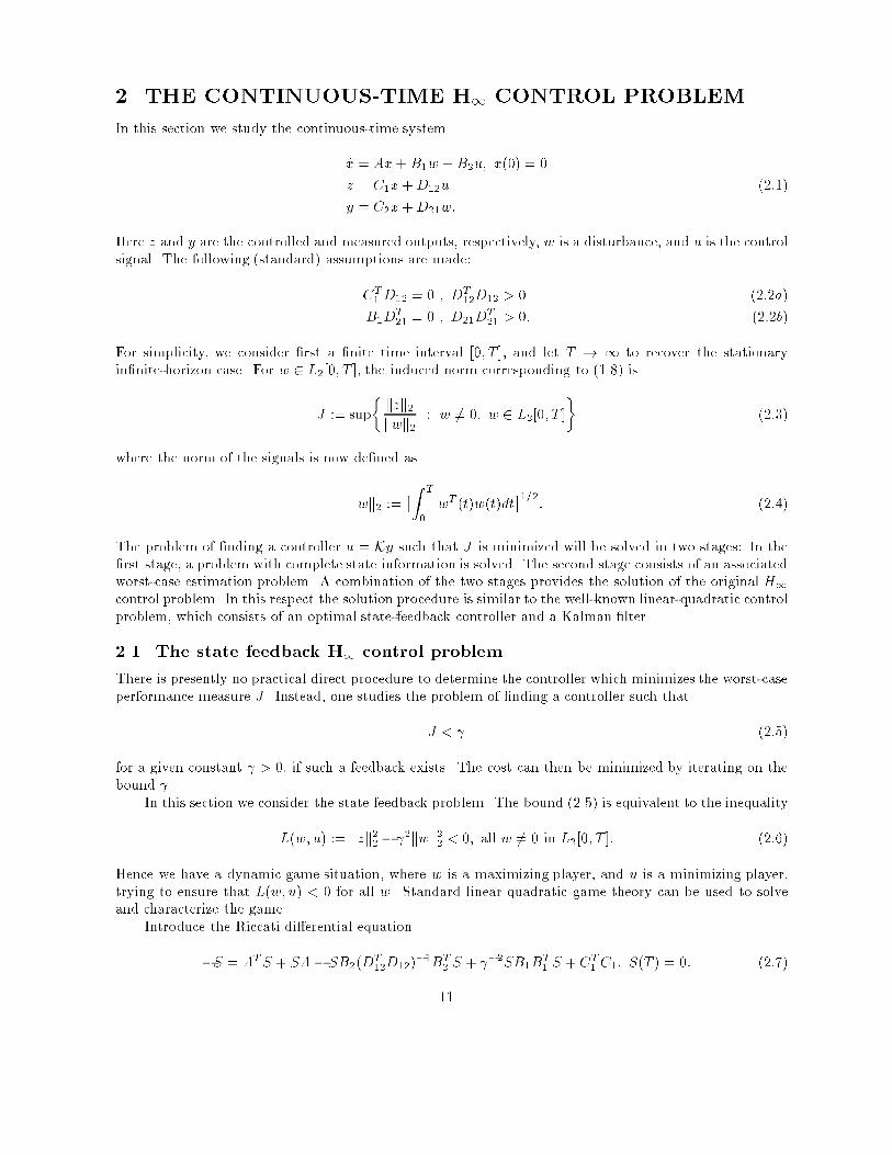
2. THE CONTINUOUS-TIME H1 CONTROL PROBLEM
In this section we study the continuous-time system
_x = Ax+ B1w + B2u; x(0) = 0
z = C1x+D12u
y = C2x+D21w:
(2:1)
Here z and y are the controlled and measured outputs, respectively, w is a disturbance, and u is the controlsignal. The following (standard) assumptions are made:
CT1 D12 = 0 ; DT
12D12 > 0 (2:2a)
B1DT21 = 0 ; D21D
T21 > 0: (2:2b)
For simplicity, we consider �rst a �nite time interval [0; T ], and let T ! 1 to recover the stationaryin�nite-horizon case. For w 2 L2[0; T ], the induced norm corresponding to (1.8) is
J := sup
� kzk2kwk2 : w 6= 0; w 2 L2[0; T ]
�(2:3)
where the norm of the signals is now de�ned as
kwk2 :=�Z T
0
wT (t)w(t)dt
�1=2: (2:4)
The problem of �nding a controller u = Ky such that J is minimized will be solved in two stages: In the�rst stage, a problem with complete state information is solved. The second stage consists of an associatedworst-case estimation problem. A combination of the two stages provides the solution of the original H1
control problem. In this respect the solution procedure is similar to the well-known linear-quadratic controlproblem, which consists of an optimal state-feedback controller and a Kalman �lter.
2.1. The state feedback H1 control problem
There is presently no practical direct procedure to determine the controller which minimizes the worst-caseperformance measure J . Instead, one studies the problem of �nding a controller such that
J < (2:5)
for a given constant > 0, if such a feedback exists. The cost can then be minimized by iterating on thebound .
In this section we consider the state feedback problem. The bound (2.5) is equivalent to the inequality
L(w; u) := kzk22 � 2kwk22 < 0; all w 6= 0 in L2[0; T ]: (2:6)
Hence we have a dynamic game situation, where w is a maximizing player, and u is a minimizing player,trying to ensure that L(w; u) < 0 for all w. Standard linear quadratic game theory can be used to solveand characterize the game.
Introduce the Riccati di�erential equation
� _S = ATS + SA � SB2(D
T12D12)
�1BT2 S +
�2SB1B
T1 S +C
T1 C1; S(T ) = 0: (2:7)
11

If (2.7) has a bounded symmetric positive semide�nite solution S(t) on [0; T ], then the quadratic functionL(w; u) can be expanded as
L(w; u) =
Z T
0
�zTz �
2wTw�dt
=
Z T
0
�(u� u
0)TDT12D12(u� u
0)� 2(w �w
0)(w �w0)�dt+ x(0)TS(0)x(0) (2:8)
where
u0(t) := �(DT
12D12)�1BT2 S(t)x(t) (2:9a)
w0(t) :=
�2BT1 S(t)x(t): (2:9b)
Eq. (2.8) shows that, provided (2.7) has a bounded solution on [0; T ], the optimal strategy for themaximizing player w is w = w
0, and likewise, the optimal strategy for the minimizing player u is u = u0.
Eq. (2.8) also shows that with the minimizing strategy u = u0, L(w; u0) � 0 (since x(0) = 0). In fact it
can be shown that L(w; u0) < 0 for all w 6= 0. It can also be shown that if the Riccati di�erential equation(2.7) has no bounded solution on [0; T ], then there exists no minimizing strategy for which L(w; u) has abounded supremum in w, and hence (2.6) cannot hold. We thus have the following result.
Theorem 2.1 There exists a state-feedback controller which achieves the performance bound (2.5), J < ,
for the system (2.1) if and only if the Riccati equation (2.7) has a bounded symmetric positive semide�nite
solution on [0; T ]. In that case, the static state feedback law (2.9a),
u(t) = �(DT12D12)
�1BT2 S(t)x(t)
achieves the performance bound (2.5).
Remark 2.1. By setting B2 = 0, Theorem 2.1 gives a test for the L2-induced norm of a linear system.The induced norm J in equation (2.3) of the system
_x = Ax+ Bw; x(0) = 0
z = Cx(2:10)
satis�es the bound J < if and only if the Riccati equation
� _S = ATS + SA +
�2SBB
TS + C
TC; S(T ) = 0 (2:11)
has a bounded symmetric positive semide�nite solution on [0; T ].
Remark 2.2. Note that in the case B1 = 0, (2.8) reduces to
Z T
0
zTzdt =
Z T
0
(u � u0)TDT
12D12(u� u0)dt+ x(0)TS2(0)x(0)
where S2(�) is now given by
� _S2 = ATS2 + S2A� S2B2(D
T12D12)
�1BT2 S2 +C
T1 C1; S2(T ) = 0 (2:12)
Thus we obtain the solution of the Linear Quadratic control problem as a special case: the minimum ofkzk22 is given by
minu
Z T
0
zTzdt = x(0)TS2(0)x(0)
and it is achieved with the control law
u0(t) := �(DT
12D12)�1BT2 S2(t)x(t)
12

where S2(�) is the solution to (2.12).
Stationary case
In the in�nite-horizon (T ! 1), time-invariant case, one would expect that the Riccati equation (2.7)reduces to a stationary algebraic Riccati equation. For this case we have the following result, which wepresent here without proof.
Theorem 2.2 Consider the system (2.1). Assume that the system is time-invariant, and
(i) (A;B2) is stabilizable,
(ii) (C1; A) is detectable.
Then the following statements are equivalent:
(a) There exists a state feedback law u = Ky such that
J := sup
� kzk2kwk2 : w 6= 0; w 2 L2[0;1)
�< (2:13)
(b) There exists a bounded symmetric positive semide�nite matrix S1 which satis�es the stationary Riccati
equation
ATS1 + S1A� S1B2(D
T12D12)
�1BT2 S1 +
�2S1B1B
T1 S1 +C
T1 C1 = 0 (2:14)
such that the closed-loop matrix
A�B2(DT12D12)
�1BT2 S1 +
�2B1B
T1 S1
is stable.
Moreover, when these conditions are satis�ed, a controller which achieves the bound in (2.13) is given
by the static constant state feedback law
u(t) = �(DT12D12)
�1BT2 S1x(t) (2:15)
The solution to the state feedback problem can be used to transform the problem of �nding a controlleru = Ky such that J < into an equivalent H1 estimation problem. Note that if we introduce the variabletransformations
v(t) := w(t)�w0(t)
= w(t)� �2BT1 S(t)x(t) (2:16a)
r(t) := (DT12D12)
1=2[u(t)� u0(t)]
= (DT12D12)
1=2u(t) + (DT
12D12)�1=2
BT2 S(t)x(t); (2:16b)
then we have from (2.8) (since x(0) = 0),
L(w; u) =
Z T
0
�zTz �
2wTw�dt =
Z T
0
�rTr �
2vTv�dt (2:17)
or,L(w; u) = kzk22 �
2kwk22 = krk22 � 2kvk22 (2:18)
From the connection between w and v it can be shown that v 6= 0 if and only if w 6= 0. Hence it followsthat
kzk22 � 2kwk22 < 0; all w 6= 0 in L2[0; T ] (2:19a)
if and only ifkrk22 �
2kvk22 < 0; all v 6= 0 in L2[0; T ] (2:19b)
13

Introducing the new variables r(t) and v(t) in the system (2.1) gives
_x(t) = [A+ �2B1B
T1 S(t)]x(t) +B1v(t) + B2u(t); x(0) = 0
r(t) = (DT12D12)
�1=2BT2 S(t)x(t) + (DT
12D12)1=2
u(t)
y(t) = [C2 + �2D21B
T1 S(t)]x(t) +D21v(t)
(2:20)
From the identity (2.19), and noting that the existence of a state feedback which achieves the bound (2.5) isa necessary condition for the existence of any controller which achieves (2.5), we have the following lemma.
Lemma 2.1 Consider the system (2.1). For any controller u = Ky, the following statements are equivalent:
(a) J < (i.e. (2.19a)) holds for the system (2.1),
(b) The Riccati di�erential equation (2.7) has a bounded symmetric positive semide�nite solution on
[0; T ], and
�J := sup
�krk2kvk2 : v 6= 0; v 2 L2[0; T ]
�< (2:21)
(i.e. (2.19b)) holds for the system (2.20).
Now a key observation is that the problem of �nding a controller u = Ky such that (2.21), �J < ,holds for the system (2.20) is equivalent to an H1-type estimation problem. This follows from the factthat the matrix (DT
12D12)1=2 in (2.20) is invertible, by assumption (2.2a). Hence it follows that if r is an
estimate of r, which is based on the measured output y and the known input u to the system, then u(t)
can always be chosen so that r � 0. Then
krk22 � 2kvk22 = kr � rk22 �
2kvk22and the problem of �nding a controller u = Ky such that (2.19b) holds can thus be solved by constructingan H1-optimal estimator for estimating r which achieves the performance bound
kr � rk22 � 2kvk22 < 0; all v 6= 0 in L2[0; T ]
and by taking u to make r � 0. We summarize the equivalence of the H1 control problem for the system(2.20) and an H1-optimal estimation problem in terms of the following lemma.
Lemma 2.2 Consider the system (2.20). There exists a causal controller u = Ky which achieves the
performance bound (2.21), �J < , if and only if there exists an estimator r which is a causal function of y
and u and which achieves the performance bound
kr� rk22 � 2kvk22 < 0; all v 6= 0 in L2[0; T ] (2:22)
Proof: First assume that there exists a controller u = Ky which achieves the performance bound (2.21).Form the causal estimator
_x(t) = �A(t)x(t) + B2[u(t)� (Ky)(t)]; x(0) = 0
r(t) = �C1(t)x(t) + (DT12D12)
1=2[u(t)� (Ky)(t)]
where
�A(t) = A + �2B1B
T1 S(t)
�C1(t) = (DT12D12)
�1=2BT2 S(t)
With u = Ky, we have r � 0, and since (2.21) holds, the estimator achieves the performance bound (2.22).From (2.20) and the structure of the estimator it is seen that u a�ects r and r in identical ways. It followsthat the estimation error is independent of u, and the estimator thus achieves the performance bound(2.22) for all inputs.
14

Conversely, assume that there exists a causal estimator r which achieves the performace bound (2.22).For (2.22) to hold for all u, the estimator must then be of the form r = F1y + F2u, where F1 is a causaloperator, and r2 := F2u is de�ned by (cf. (2.20))
_x2(t) = �A(t)x2(t) +B2u(t)
r2(t) = �C1(t)x2(t) + (DT12D12)
1=2u(t):
As D12 has full row rank the control signal can now be chosen so that r2 = �F1y, and hence r � 0. Thenr � r � r, and the controller constructed in this way achieves the performance bound (2.21), because theestimator achieves the bound (2.22).
Lemma 2.1 and Lemma 2.2 show that in order to solve the general H1 control problem, we are led tostudy an H1-optimal estimation problem.
2.2. An H1 estimation problem
In this section we study the system
_x = Ax+B1w; x(0) = 0
z = C1x
y = C2x+D21w
(2:23)
where we assume (cf. Eq. (2.2b))
B1DT21 = 0 (2:24a)
D21DT21 > 0 (2:24b)
These asumptions, as well as the zero initial state assumption x(0) = 0, can be easily relaxed, but here weshall only consider the somewhat simpler case (2.23), (2.24).
The problem is to estimate the signal z using measurements y in such a way that a worst-caseperformance bound is satis�ed. More speci�cally, we introduce the induced norm from the disturban-ce w 2 L2[0; T ] to the estimation error z � z 2 L2[0; T ],
Je := sup
�kz � zk2kwk2 : w 6= 0; w 2 L2[0; T ]
�(2:25)
Then the performance boundJe < (2:26)
for a given constant > 0 is equivalent to the quadratic bound
Le(w; z) := kz � zk22 � 2kwk22 < 0; all w 6= 0 in L2[0; T ]; (2:27)
cf. (2.5) and (2.6).The H1 estimation problem will be solved by taking it into an equivalent (dual) state feedback
problem, which can then be solved using the approach described in Section 2.1.In order to derive the equivalent dual state feedback problem, it is convenient to describe the problem
using operator notation. LetG1;G2 : L2[0; T ]! L2[0; T ] (2:28)
denote the linear operators de�ned by (2.23) which take the disturbance w to the outputs z and y, respec-tively, so that �
z
y
�=
�G1G2�w (2:29)
15

The operators G1 and G2 are, of course, explicitly given by
(G1w)(t) =Z t
0
C1�A(t; �)B1w(�)d� (2:30a)
(G2w)(t) =Z t
0
C2�A(t; �)B1w(�)d�+D21w(t) (2:30a)
where �A(�; �) is the state transition matrix associated with the system matrix A, see Appendix A.Assume that we have the linear estimator
z = Fy (2:31)
where F : L2[0; T ] ! L2[0; T ] is a linear and causal operator. By (2.29) and (2.31) we have for theestimation error,
z � z = G1w �Fy = [G1 �FG2]w (2:32)
The induced operator norm in (2.32) is given as
kG1 �FG2k := sup
�k[G1� FG2]wk2kwk2 : w 6= 0; w 2 L2[0; T ]
��
= sup
�kz � zk2kwk2 : w 6= 0; w 2 L2[0; T ]
�= Je (2:33)
Hence the performance bound (2.21), Je < , can be expressed in terms of the operator norm as
kG1 � FG2k < (2:34)
In terms of the adjoint operator (see Appendix B), we have
k(G1 � FG2)�k = kG1 �FG2k (2:35)
Here(G1 �FG2)� = G�1 � G�2F�
Hence (2.34) is equivalent tokG�1 � G�2F�k < (2:36)
Now consider the adjoint operator
[G�1 G�2 ] : L2[0; T ]� L2[0; T ]! L2[0; T ] (2:37)
and let
s = [G�1 G�2 ]��
�
�; �; � 2 L2[0; T ] (2:38)
Using the control law� = �F��; (2:39)
the signal s is given bys = (G�1 � G�2F�)� (2:40)
and the norm bound (2.36) is equivalent to the worst-case performance bound
sup
�ksk2k�k2 : � 6= 0; � 2 L2[0; T ]
�< (2:41)
16
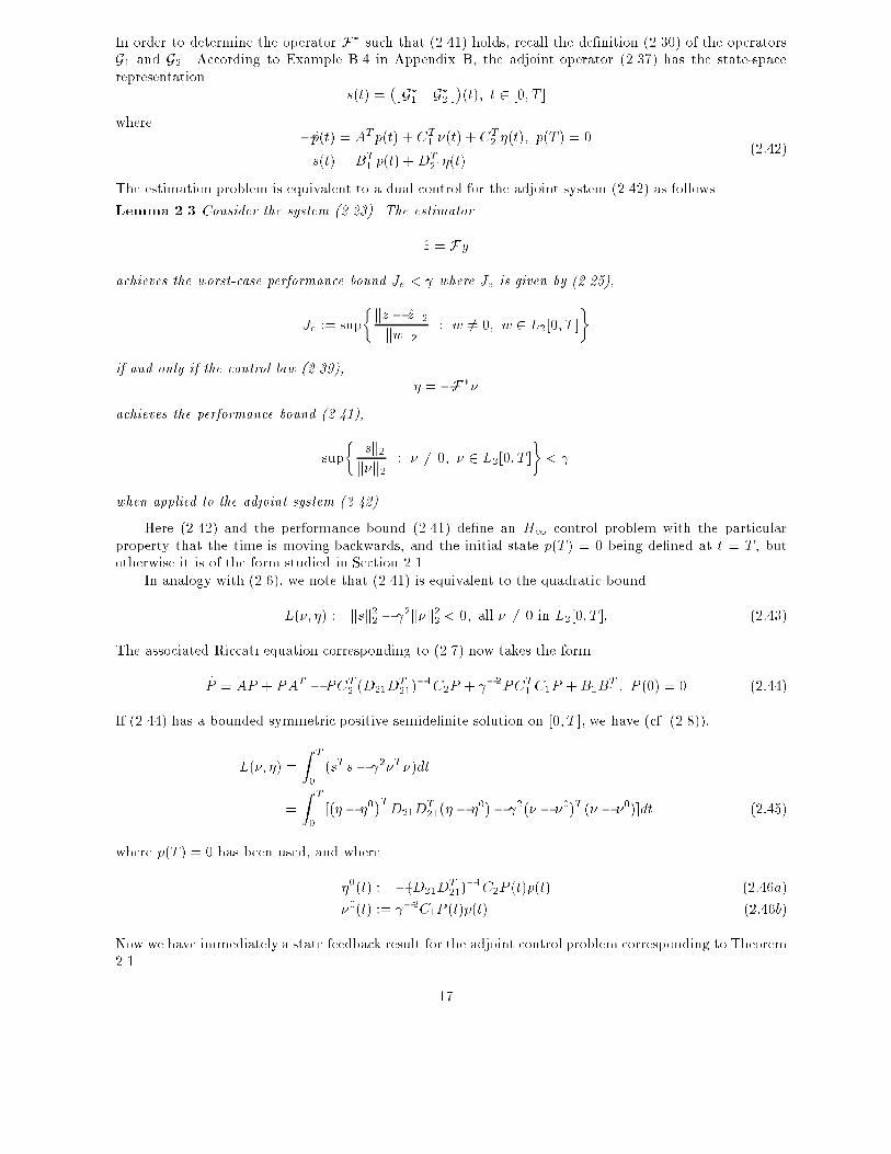
In order to determine the operator F� such that (2.41) holds, recall the de�nition (2.30) of the operatorsG1 and G2. According to Example B.4 in Appendix B, the adjoint operator (2.37) has the state-spacerepresentation
s(t) =�[G�1 G�2 ]
�(t); t 2 [0; T ]
where� _p(t) = A
Tp(t) +C
T1 �(t) +C
T2 �(t); p(T ) = 0
s(t) = BT1 p(t) +D
T21�(t)
(2:42)
The estimation problem is equivalent to a dual control for the adjoint system (2.42) as follows.
Lemma 2.3 Consider the system (2.23). The estimator
z = Fy
achieves the worst-case performance bound Je < where Je is given by (2.25),
Je := sup
�kz � zk2kwk2 : w 6= 0; w 2 L2[0; T ]
�
if and only if the control law (2.39),
� = �F��achieves the performance bound (2.41),
sup
� ksk2k�k2 : � 6= 0; � 2 L2[0; T ]
�<
when applied to the adjoint system (2.42).
Here (2.42) and the performance bound (2.41) de�ne an H1 control problem with the particularproperty that the time is moving backwards, and the initial state p(T ) = 0 being de�ned at t = T , butotherwise it is of the form studied in Section 2.1.
In analogy with (2.6), we note that (2.41) is equivalent to the quadratic bound
L(�; �) := ksk22 � 2k�k22 < 0; all � 6= 0 in L2[0; T ]; (2:43)
The associated Riccati equation corresponding to (2.7) now takes the form
_P = AP + PAT � PC
T2 (D21D
T21)
�1C2P +
�2PC
T1 C1P +B1B
T1 ; P (0) = 0 (2:44)
If (2.44) has a bounded symmetric positive semide�nite solution on [0; T ], we have (cf. (2.8)),
L(�; �) =
Z T
0
(sT s � 2�T�)dt
=
Z T
0
[(� � �0�TD21D
T21
�� � �
0)� 2(� � �
0)T (� � �0)]dt (2:45)
where p(T ) = 0 has been used, and where
�0(t) := �(D21D
T21)
�1C2P (t)p(t) (2:46a)
�0(t) :=
�2C1P (t)p(t) (2:46b)
Now we have immediately a state feedback result for the adjoint control problem corresponding to Theorem2.1.
17

Lemma 2.4 Consider the adjoint system (2.42). There exists a state feedback which achieves the perfor-
mance bound (2.41) if and only if the Riccati equation (2.44) has a bounded symmetric positive semide�nite
solution on [0; T ]. In that case, the static state feedback
�(t) = �(D21DT21)
�1C2P (t)p(t)
achieves the bound (2.41).
In order to characterize the dual control problem in Lemma 2.3, note that the state p(t) is exactlyreconstructable from � and �. This gives us the following solution to the dual control problem.
Lemma 2.5 Consider the adjoint system (2.42). There exists an anticausal control law � = �F�� which
achieves the performance bound (2.41) if and only if the Riccati di�erential equation (2.44) has a bounded
symmetric positive semide�nite solution on [0; T ]. In that case, the controller described by the state-space
equations
� _p(t) = ATp(t) + C
T1 �(t) + C
T2 �(t); p(T ) = 0
�(t) = �(D21DT21)
�1C2P (t)p(t)
(2:47)
achieves the bound (2.41).
Proof: The result follows from Lemma 2.4 by observing that p(t) = p(t), all t 2 [0; T ]. Note also that thecontroller � = �F�� de�ned by (2.47) is anticausal.
We can now apply Lemma 2.3 to construct an estimator z = Fy which achieves the speci�ed perfor-mance bound for the system (2.23). First note that � = �F�� in (2.47) may be written as
� _p(t) = ATp(t) +C
T1 �(t)�C
T2 (D21D
T21)
�1C2P (t)p(t)
= [A� P (t)CT2 (D21D
T21)
�1C2]
Tp(t) + C
T1 �(t); p(T ) = 0
�(t) = �(D21DT21)
�1C2P (t)p(t)
(2:48)
By Example B.4, the �lter z = Fy corresponding to (2.48) is then given by
_x(t) = [A� P (t)CT2 (D21D
T21)
�1C2]x(t) + P (t)CT
2 (D21DT21)
�1y(t)
z(t) = C1x(t) ; x(0) = 0
or,_x(t) = Ax(t) + P (t)CT
2 (D21DT21)
�1[y(t) �C2x(t)]
z(t) = C1x(t) ; x(0) = 0
To summarize, we have the following theorem.
Theorem 2.3 Consider the system (2.23). There exists an estimator z = Fy which achieves the perfor-
mance bound (2.26), Je < , if and only if the Riccati di�erential equation (2.44) has a bounded symmetric
positive semide�nite solution on [0; T ]. In this case, the �lter
_x(t) = Ax(t) + P (t)CT2 (D21D
T21)
�1[y(t) �C2x(t)]
z(t) = C1x(t) ; x(0) = 0(2:49)
achieves the performance bound (2.26).
It is interesting to note that the estimator (2.49) has the same structure as the well-known Kalman�lter. Moreover, it can be seen from the Riccati equation (2.44) that the estimator reduces to the Kalman�lter in the limiting case 2 !1.
2.3. Solution of the H1 control problem
Now we return to the problem of �nding a causal controller u = Ky for the system (2.1) such that theworst-case performance bound (2.5) is achieved.
18

Recall the variable transformation (2.16), which, when introduced in the system equations (2.1), gives(2.20), or
_x(t) = �A(t)x(t) +B1v(t) + B2u(t); x(0) = 0
r(t) = �C1(t)x(t) + (DT12D12)
1=2u(t)
y(t) = �C2(t)x(t) +D21v(t)
(2:50)
where
�A(t) = A+ �2B1B
T1 S(t) (2:51a)
�C1(t) = (DT12D12)
�1=2BT2 S(t) (2:51b)
�C2(t) = C2 + �2D21B
T1 S(t) = C2 (2:51c)
Here we have used assumption (2.2b) in Eq. (2.51c). In Section 2.1 it was also shown (Lemma 2.1) that theperformance bound (2.5), J < , holds for the system (2.1) if and only if the performance bound (2.21),�J < , holds for the system (2.20), and that the resulting H1 control problem is equivalent to an H1
estimation problem (Lemma 2.2). Lemma 2.2 and the estimation results in Section 2.2 can be combinedto give the following lemma.
Lemma 2.6 Consider the system (2.50). The following statements are equivalent:
(i) There exists a causal controller u = Ky such that the performance bound (2.21),
�J := sup
�krk2kvk2 : v 6= 0; v 2 L2[0; T ]
�<
is achieved;
(ii) There exists a causal estimator r = Fy such that
sup
�kr � rk2kvk2 : v 6= 0; v 2 L2[0; T ]
�<
(iii) There exists a bounded symmetric positive semide�nite solution Q(t) on [0; T ] to the Riccati di�erential
equation
_Q(t) = �A(t)Q(t) + Q(t) �AT (t) �Q(t) �CT2 (t)(D21D
T21)
�1 �C2(t)Q(t) + �2Q(t) �C1(t)
T �C1(t)Q(t) +B1BT1 ;
Q(0) = 0 (2:52)
Moreover, when these conditions are satis�ed, a controller which achieves the performance bound �J <
is given by
_x(t) = �A(t)x(t) +B2u(t) +Q(t) �CT2 (t)(D21D
T21)
�1[y(t) � �C2(t)x(t)]; x(0) = 0
u(t) = �(DT12D12)
�1=2 �C1(t)x(t)(2:53)
Note that the control signal u sets the estimate r = 0, cf. the proof of Lemma 2.2. By equation (2.51b),the expression for u(t) in (2.53) may also be written as
u(t) = �(DT12D12)
�1BT2 S(t)x(t)
The results so far can be summarized as follows.
Theorem 2.4 Consider the system (2.1). There exists a causal controller u = Ky such that the performance
bound (2.5), J < , holds if and only if the following conditions are satis�ed:
(a) The Riccati di�erential equation (2.7),
� _S = ATS + SA � SB2(D
T12D12)
�1BT2 S +
�2SB1B
T1 S +C
T1 C1; S(T ) = 0
19

has a bounded symmetric positive semide�nite solution on [0; T ].
(b) The Riccati di�erential equation (2.52) has a bounded symmetric positive semide�nite solution on
[0; T ].
Moreover, when these conditions hold, a controller which achieves the performance bound J < is
given by Eq. (2.53).
Remark 2.3. Note that (a) is a necessary and su�cient condition for the existence of a state feedback whichachieves the performance bound J < (Theorem 2.1), while (b) is a necessary and su�cient condition forthe existence of an estimator which achieves the worst-case performance bound (2.21) for the transformedsystem (2.20).
The H1 optimal controller (2.53) is thus obtained in terms of the two coupled Riccati equations (2.7)for S(�) and (2.52) for Q(�). (Note that Q(t) depends on S(t) via the matrices in (2.20).) Remarkably,however, it turns out that it is su�cient to solve two uncoupled Riccati di�erential equations associatedwith the system (2.1). This follows from the following connection which exists between the solutions S(�)of (2.7), P (�) of (2.44) and Q(�) of (2.52).Theorem 2.5 Assume that the Riccati di�erential equation (2.7),
� _S = ATS + SA � SB2(D
T12D12)
�1BT2 S +
�2SB1B
T1 S + C
T1 C1; S(T ) = 0 [(2:7)]
has a bounded symmetric positive semide�nite solution on [0; T ]. Then the Riccati di�erential equation
(2.52),
_Q(t) = �A(t)Q(t) +Q(t) �AT (t)� Q(t) �CT2 (t)(D21D
T21)
�1 �C2(t)Q(t) + �2Q(t) �C1(t) �C
T1 (t)Q(t) + B1B
T1 ;
Q(0) = 0; [(2:52)]
where (cf. (2.51)),
�A(t) = A+ �2B1B
T1 S(t)
�C1(t) = (DT12D12)
�1=2BT2 S(t)
�C2(t) = C2 + �2D21B
T1 S(t) = C2
has a bounded symmetric positive semide�nite solution on [0; T ] if and only if the following conditions are
satis�ed:
(a) The Riccati di�erential equations (2.44),
_P = AP + PAT � PC
T2 (D21D
T21)
�1C2P +
�2PC
T1 C1P + B1B
T1 ; P (0) = 0 [(2:44)]
has a bounded symmetric positive semide�nite solution on [0; T ], and
(b) �(S(t)P (t)) < 2, all t 2 [0; T ], where �(�) denotes the spectral radius of a matrix; �(�) := maxfj�(�)jg.
Moreover, when conditions (a) and (b) are satis�ed, then the matrix Q(t) of Eq. (2.52) is given by
Q(t) = P (t)�I �
�2S(t)P (t)
��1; t 2 [0; T ]: (2:54)
Proof: Assume that (2.52) has a bounded symmetric positive semide�nite solution Q(t). Then it is easyto verify that the matrix P (t) := Q(t)(I +
�2S(t)Q(t))�1 is symmetric and positive semide�nite, satis�es
(2.44), and that (2.54) holds. Moreover, we have (cf. Lemma 2.7)
�(SP ) = ��SQ(I +
�2SQ)�1
�=
2��SQ( 2I + SQ)�1
�<
2:
Hence (b) holds. Conversely, assume that (a) and (b) hold. Then it is straightforward to verify that thematrix Q(t) de�ned by Eq. (2.54) is symmetric, positive semide�nite, and satis�es the Riccati di�erentialequation (2.52).
We have above made use of the following result.
20

Lemma 2.7 Let S and Q be symmetric, positive semide�nite matrices. Then
��SQ( 2I + SQ)�1
�=
�(SQ)
2 + �(SQ)< 1:
Combining Theorems 2.4 and 2.5 gives the following result for the existence of a controller satisfyinga closed-loop bound on the L2-induced norm.
Theorem 2.6 Consider the system (2.1). Assume that assumptions (2.2) hold. There exists a controller
u = Ky which achieves the performance bound (2.5), J < , if and only if the following conditions are
satis�ed:
(a) The Riccati di�erential equation (2.7),
� _S = ATS + SA � SB2(D
T12D12)
�1BT2 S +
�2SB1B
T1 S +C
T1 C1; S(T ) = 0 [(2:7)]
has a bounded symmetric positive semide�nite solution on [0; T ];
(b) The Riccati di�erential equation (2.44),
_P = AP + PAT � PC
T2 (D21D
T21)
�1C2P +
�2PC
T1 C1P + B1B
T1 ; P (0) = 0 [(2:44)]
has a bounded symmetric positive semide�nite solution on [0; T ];
(c) �(S(t)P (t)) < 2, all t 2 [0; T ].
Moreover, when these conditions are satis�ed, a controller which achieves the performance bound J <
is given by (2.53),
_x(t) = �A(t)x(t) +B2u(t) +Q(t) �CT2 (t)(D21D
T21)
�1[y(t) � �C2(t)x(t)]; x(0) = 0
u(t) = �(DT12D12)
�1BT2 S(t)x(t)
where we have�A(t) = A+
�2B1B
T1 S(t)
�C2(t) = C2 + �2D21B
T1 S(t) = C2
and
Q(t) = P (t)�I �
�2S(t)P (t)
��1Remark 2.4. Note that the solution has the same structure as the optimal LQ controller. In both cases thecontroller is obtained in terms two Riccati equations associated with the optimal state feedback problemand an optimal estimation problem, respectively. In Theorem 2.6,
- (a) is a necessary and su�cient condition for the existence of a state feedback such that J <
(Theorem 2.1),- (b) is a necessary and su�cient condition for the existence of an estimator for estimating the controlledsignal z such that Je < (Theorem 2.3), and
- (c) represents a coupling condition, which is necessary and su�cient for simultaneous control andestimation to achieve the performance bound J < .
Stationary case
It is of particular interest to study the in�nite-horizon case (T ! 1) for time-invariant systems. Thenthe Riccati di�erential equations (2.7) and (2.44) reduce to stationary algebraic Riccati equations. In thestationary, time-invariant case we make the following assumptions:
(A.1) The pair (A;B2) is stabilizable and the pair (C2; A) is detectable.(A.2) The pair (A;B1) is stabilizable and the pair (C1; A) is detectable.
We then have the following result.
21

Theorem 2.7 Consider the system (2.1). Assume that the system matrices are time-invariant, and that
assumptions (2.2) and (A.1), (A.2) hold. Then there exists a controller u = Ky which internally stabilizes
the system (2.1) and achieves the H1 performance bound
J := sup
� kzk2kwk2 : w 6= 0; w 2 L2[0;1)
�<
if and only if the following conditions are satis�ed:
(a) The algebraic Riccati equation
ATS1 + S1A� S1B2(D
T12D12)
�1BT2 S1 +
�2S1B1B
T1 S1 +C
T1 C1 = 0
has a bounded symmetric positive semide�nite solution S1 such that the (closed-loop) matrix
A�B2(DT12D12)
�1BT2 S1 +
�2B1B
T1 S1
is stable;
(b) The algebraic Riccati equation
AP1 + P1AT � P1C
T2 (D21D
T21)
�1C2P1 +
�2P1C
T1 C1P1 + B1B
T1 = 0
has a bounded symmetric positive semide�nite solution on P1 such that the (closed-loop) matrix
A � P1CT2 (D21D
T21)
�1C2 +
�2P1C
T1 C1
is stable;
(c) �(S1P1) < 2.
Moreover, when these conditions are satis�ed, an internally stabilizing time-invariant controller which
achieves the performance bound J < is given by
_x(t) = [A+ �2B1B
T1 S1 �B2(D
T12D12)
�1BT2 S1]x(t)
+ P1(I � �2S1P1)�1CT
2 (D21DT21)
�1�y(t) �C2(t)x(t)
�;
u(t) = �(DT12D12)
�1BT2 S1x(t)
By Theorem 2.7, a controller which achieves the performance bound J < for the stationary H1-optimal control problem can be found by checking the solution of two algebraic Riccati equations, andthe coupling condition (c). This solution to the H1 control problem was introduced by Glover and Doyle(1988), and it is commonly referred to as the �Glover-Doyle� approach, or the �two-Riccati equation�approach. An implementation of the procedure can be found in Matlab's Robust Control Toolbox (Chiangand Safonov 1988).
In order to construct a controller which minimizes the worst-case performance measure J , one cancheck the conditions of Theorem 2.7 for successively smaller values of . In this way one can determinethe quantity
inf := inf� > 0 : J < for some stabilizing controller u = Ky (2:55)
to any desired degree of accuracy. This procedure in H1 synthesis is known as � -iteration�.
Remark 2.5. Note that as !1,- the Riccati equation for S (S1) reduces to the Riccati equation in the LQ control problem,- the Riccati equation for P (P1) reduces to the Riccati equation of a Kalman �lter,- the coupling condition (c) becomes redundant, and- the controller in Theorem 2.6 (Theorem 2.7) reduces to the optimal LQG control law.
2.4. Notes and references
The connection between the H1 problem and linear quadratic game theory was �rst observed by Petersen(1987), and the stationary state feedback H1 problem was then solved in the papers by Khargonekar,
22

Petersen and Rotea (1988) and Zhou and Khargonekar (1988). The general state-space solution to thestationary H1 control problem (Theorem 2.7) was �rst given by Glover and Doyle (1988), and developedin full in the classic, hard-to-read, paper by Doyle, Glover, Khargonekar and Francis (Doyle et al. 1989),a preliminary conference version of which can be found in Doyle et al. (1988). The state-space solutionimplied a signi�cant simpli�cation in the H1 control theory. For example, the solution shows that theoptimal controller order is not higher than the order of the plant, a question which was not fully settledbefore the state-space solution was available. The �nite-horizon, time-varying problem was solved usingstate-space methods by Tadmor (1990), and Limebeer et al. (1992). The approach used here is based on atutorial paper by Limebeer and Green (1991).
The solution of the H1-optimal �ltering problem has been given in the hard-to-read paper by Nag-pal and Khargonekar (1991). An alternative (and simpler) derivation is given by Banavar and Speyer(1991). The approach used here (Section 2.2) draws from the H1 control literature, but has not appearedindependently in an H1 estimation context.
The state-space approach to H1 control is discussed in a number of books which have appearedrecently. A thorough coverage of robust control is provided by the book by Green and Limebeer (1995).The book by Ba�sar and Bernhard (1991) gives an in depth presentation of the game-theory approach toH1 control. Stoorvogel (1992) presents a closely related approach where the results are derived using linearoptimal control theory and the maximum principle. Useful material can also be found in McFarlane andGlover (1990). The Glover-Doyle approach is mentioned in Maciejowski (1989), and an implementationcan be found in Matlab's Robust Control Toolbox. The standard reference in linear-quadratic games, withwhich the state-space H1 solution is closely related, is the book by Ba�sar and Olsder (1982).
PROBLEMS
2.1. Show Eq. (2.8).
2.2. Consider the scalar system_x = ax+ bw; x(0) = 0
z = cx
Find an analytical solution to the Riccati equation (2.11), and study how it behaves as is decreased (andJ < does not hold any more).
Show that as T !1, (2.10) approaches a stationary solution, provided is su�ciently large.
2.3. Consider the scalar system
_x = ax+ b1w + +b2u; x(0) = 0
z = C1x+D12u
where
a = 1; b1 = 1; b2 = 2; C1 =
�1
0
�D12 =
�0
1
�:
Find a state feedback which minimizes the L2-induced norm
J := sup
� R10
zT (t)z(t)dtR1
0wT (t)w(t)dt
: w 6= 0; w 2 L2[0;1)
�
of the closed-loop system.
2.4. Consider the scalar system in Problem 2.2, and the stationary version of the associated Riccatiequation (2.11). Show that for a stable system (a < 0), and with > inf , where
inf := J = sup�kzk2=kwk2 : w 6= 0; w 2 L2[0;1)
the Riccati equation has two positive solutions, but only one of these satis�es the closed-loop stabilitycondition in Theorem 2.2. Compare the solution with the limiting solution obtained in Problem 2.2.
23

Study also the stationary Riccati equation in the following cases:- = inf ,- < inf ,- a � 0.
Comment your �ndings!
2.5. Study the stationary Riccati equation (2.14) associated with the scalar system
_x = ax+ b1w + +b2u; x(0) = 0
z = C1x+D12u
where
C1 =
�c
0
�D12 =
�0
1
�:
Show in particular that there are cases when the Riccati equation (2.14) has two positive solutions, only oneof which satis�es the stability condition stated in Theorem 2.2. Verify that the solution which satisifes thestability condition is the smallest positive solution of the Riccati equation. Show also that both positivesolutions of the Riccati equation (2.14) have the property that the state feedback (2.15) gives a stableclosed-loop system which achieves the performance bound (2.13).
2.6. Show the "push-through"-identity
A(I + BA)�1 = (I +AB)�1A
where A and B are operators on appropriate spaces (or matrices of appropriate dimensions) and I is theidentity operator (matrix).
2.7. (Theorem 2.5) Assume that Equation (2.7) has a bounded solution S(t) and that (2.52) has a boundedsolution Q(t). Show that the matrix
P (t) := Q(t)�I +
�2S(t)Q(t)
��1is a solution to (2.44).
2.8. (Lemma 2.7) Prove Lemma 2.7 in the following steps:(i) Show that with M := SQ, � is an eigenvalue of M ( 2I + M )�1 if and only if 2�=(1 + �) is an
eigenvalue of M .(ii) Show that for symmetric, positive de�nite matrices S and Q, the eigenvalues of M := SQ are non-
negative. (Hint: Show that if � is an eigenvalue of SQ, then it is also an eigenvalue of Q1=2SQ
T=2,where Q = Q
T=2Q1=2, and hence nonnegative.)
(iii) Show that Lemma 2.7 follows from (i) and (ii).
2.9. Consider the system described by Equation (2.1) with
A =
24 0 1 0
0 �0:1 0
1 0 �0:2
35 ; B1 =
24 0:4 0
1 0
0 0
35 ; B2 =
240
1
0
35
C1 =
�0 0 1
0 0 0
�; D12 =
�0
0:5
�C2 = [ 1 0 0 ] ; D21 = [ 0 0:1 ]
a) Determine inf of the stationary H1-optimal control problem, and �nd a controller which achieves theperformance bound J < := inf + �, for some small � > 0.b) plot the singular values
�k(Tzw(i!))
24
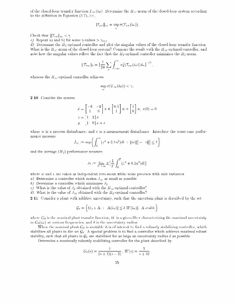
of the closed-loop transfer function Tzw(i!). Determine the H1-norm of the closed-loop system accordingto the de�nition in Equation (1.7), i.e.,
kTzwk1 = sup!
��(Tzw(i!)):
Check that kTzwk1 < .c) Repeat a) and b) for some -values > inf .d) Determine the H2-optimal controller and plot the singular values of the closed-loop transfer function.What is the H1-norm of the closed-loop system? Compare the result with the H1-optimal controller, andnote how the singular values re�ect the fact that the H2-optimal controller minimizes the H2-norm,
kTzwk2 =� 1
2�
Xk
Z 1
�1
�2k(Tzw(i!))d!
�1=2;
whereas the H1-optimal controller achieves
sup!
��(Tzw(i!)) < :
2.10. Consider the system
_x =
��3 �21 0
�x+
�0:5
1
�w +
�1
0
�u; x(0) = 0
z = [1 2 ]x
y = [1 0 ]x+ v
where w is a process disturbance, and v is a measurement disturbance. Introduce the worst-case perfor-mance measure
J1 := sup
�Z 1
0
(z2 + 0:1u2)dt : kwk22 + kvk22 � 1
�
and the average (H2) performance measure
J2 := limT!1
E� 1T
Z T
0
(z2 + 0:1u2)dt
where w and v are taken as independent zero-mean white noise proceses with unit variances.a) Determine a controller which makes J1 as small as possible.b) Determine a controller which minimizes J2.c) What is the value of J2 obtained with the H1-optimal controller?d) What is the value of J1 obtained with the H2-optimal controller?
2.11. Consider a plant with additive uncertainty, such that the uncertain plant is described by the set
G� =nG0 +� : j�(i!)j � �jW (i!)j; � stable
owhere G0 is the nominal plant transfer function, W is a given �lter characterizing the maximal uncertaintyin G0(i!) at various frequencies, and � is the uncertainty radius.
When the nominal plant G0 is unstable it is of interest to �nd a robustly stabilizing controller, whichstabilizes all plants in the set G�. A special problem is to �nd a controller which achieves maximal robuststability, such that all plants in G� are stabilized for as large an uncertainty radius � as possible.
Determine a maximally robustly stabilizing controller for the plant described by
G0(s) =1
(s + 1)(s+ 3); W (s) =
2
s + 10:
25

What is the maximal uncertainty radius for which this controller achieves robust stability?
2.12. (Relaxation of orthogonality assumption.) Consider a system described by equation (2.1), butwithout requiring that the orthogonality relation in (2.2a) holds, i.e., we may have CT
1 D12 6= 0.a) Show by a completion of squares argument that
zTz = x
T ~C1~CT1 x+ ~uTDT
12D12~u
where~C1
~CT1 := C
T1 (I �D12(D
T12D12)
�1DT12)C1
and~u := u+ (DT
12D12)�1DT12C1x
b) Using the result above we can de�ne the new varibles ~u and
~z :=
�~C1
0
�x+
�0
D12
�~u
Then zTz = ~zT ~z, and the L2-induced norm is not a�ected by the variable change. In the new variables,
the orthogonality assumption in (2.2a) holds, and hence the results obtained for this case can be used.Show that the optimal state feedback of Theorem 2.1 is then replaced by the feedback law
u(t) = �(DT12D12)
�1(BT2 S(t) +D
T12C1)x(t)
where S(�) is a solution to
� _S = ~ATS + S ~A � SB2(D
T12D12)
�1BT2 S +
�2SB1B
T1 S + ~CT
1~C1; S(T ) = 0
where ~A := A�B2(DT12D12)
�1DT12C1.
c) Show that the Riccati equation above can be written in the form
� _S = ATS + SA � (SB2 +C
T1 D12)(D
T12D12)
�1(BT2 S +D
T12C1) +
�2SB1B
T1 S +C
T1 C1
REFERENCES
Banavar, R. N., and J. L. Speyer (1991). �A Linear Quadratic GameApproach to Estimation and Smoothing,�Proceedings of the 1991 American Control Conference, pp. 2818�2822, Boston.
Ba�sar, T., and P. Bernhard (1991). H1 Optimal Control and Related Minimax Design Problems: A Dy-
namic Game Approach, Birkhauser, Boston.Ba�sar, T., and G. J. Olsder (1982). Dynamic Noncooperative Game Theory, Academic Press, London/New
York.Chiang, R. Y., and M. G. Safonov (1988) Robust Control Toolbox, The MathWorks, Inc..Doyle, J., K. Glover, P. Khargonekar, and B. Francis (1988). �State-Space Solutions to Standard H2 and
H1 Control Problems,� Proceedings of the 1988 American Control Conference, 1691�1696.Doyle, J. C., K. Glover, P. P. Khargonekar, and B. A. Francis (1989). �State-Space Solutions to Standard
H2 and H1 Control Problems,� IEEE Trans. Automat. Control 34, 831�847.Glover, K., and J. C. Doyle (1988). �State-Space Formulae for all Stabilizing Controllers that Satisfy an
H1-Norm Bound and Relations to Risk Sensitivity,� Systems & Control Letters 11, 167�172.Green, M., and D. J. N. Limebeer (1995). Linear Robust Control, Prentice-Hall, Englewood Cli�s.Khargonekar, P. P., I. R. Petersen, and M. A. Rotea (1988). �H1-Optimal Control with State Feedback,�
IEEE Trans. Automat. Control 33, 786�788.Limebeer, D. J. N., and M. Green (1991). �A GameTheoretic Approach to H1 Control,� Proc. Symposium
on Robust Control System Design Using H1 and Related Methods, Camridge, U.K.
26
Limebeer, D. J. N., B. D. O. Anderson, P. P. Khargonekar, and M. Green (1992). �A Game TheoreticApproach to H1 Control for Time-Varying Systems,� SIAM J. Control and Optimization 30, 262�283.
Maciejowski, J. M. (1989). Multivariable Feedback Design, Addison-Wesley.McFarlane, D. C., and K. Glover (1990). Robust Controller Design Using Normalized Coprime Factor Plant
Descriptions, Springer-Verlag, Berlin.Nagpal, K. M., and P. P. Khargonekar (1991). �Filtering and Smoothing in an H1 Setting,� IEEE Trans.
Automat. Control 36, 152�166.Petersen, I. R. (1987). �Disturbance Attenuation and H1 Optimizations: A Design Method Based on the
Algebraic Riccati Equation,� IEEE Trans. Automat. Control 32, 427�429.Stoorvogel, A. A. (1992). The H1 Control Problem: A State Space Approach, Prentice-Hall, Englewood
Cli�s.Tadmor, G. (1990). �Worst-Case Design in the Time Domain: The Maximum Principle and the Standard
H1 Problem,� Math. Control Signals Systems 3, pp. 301�324.Zhou, K. and P. P. Khargonekar (1988). �An Algebraic Riccati Equation Approach to H1 Optimization,�
Systems & Control Letters 11, 85�92.
27
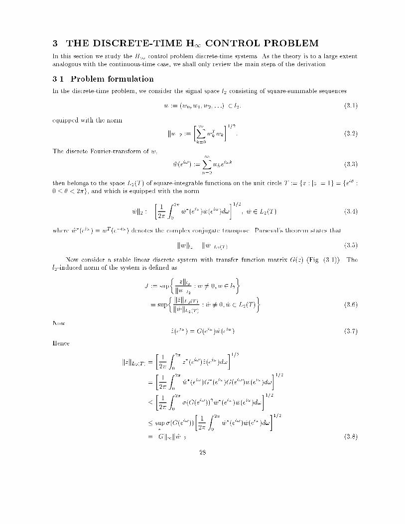
3. THE DISCRETE-TIME H1 CONTROL PROBLEM
In this section we study the H1 control problem discrete-time systems. As the theory is to a large extentanalogous with the continuous-time case, we shall only review the main steps of the derivation.
3.1. Problem formulation
In the discrete-time problem, we consider the signal space l2 consisting of square-summable sequences
w := (w0; w1; w2; : : :) 2 l2: (3:1)
equipped with the norm
kwk2 :=� 1Xk=0
wTkwk
�1=2: (3:2)
The discrete Fourier-transform of w,
w(ei!) :=
1Xk=0
wkei!k (3:3)
then belongs to the space L2(T ) of square-integrable functions on the unit circle T := fz : jzj = 1g = fei� :0 � � < 2�g, and which is equipped with the norm
kwk2 :=�1
2�
Z 2�
0
w�(ei!)w(ei!)d!
�1=2; w 2 L2(T ) (3:4)
where w�(ei!) = wT (e�i!) denotes the complex conjugate transpose. Parseval's theorem states that
kwkl2 = kwkL2(T ) (3:5)
Now consider a stable linear discrete system with transfer function matrix G(z) (Fig. (3.1)). Thel2-induced norm of the system is de�ned as
J := sup
� kzkl2kwkl2
: w 6= 0; w 2 l2
�
= sup
� kzkL2(T )kwkL2(T )
: w 6= 0; w 2 L2(T )
�(3:6)
Nowz(ei!) = G(ei!)w(ei!) (3:7)
Hence
kzkL2(T ) =�1
2�
Z 2�
0
z�(ei!)z(ei!)d!
�1=2
=
�1
2�
Z 2�
0
w�(ei!)G�(ei!)G(ei!)w(ei!)d!
�1=2
��1
2�
Z 2�
0
��(G(ei!))2w�(ei!)w(ei!)d!
�1=2
� sup!
��(G(ei!))
�1
2�
Z 2�
0
w�(ei!)w(ei!)d!
�1=2= kGk1kwk2 (3:8)
28

where we have introduced the H1-norm
kGk1 := sup!
��(G(ei!)) (3:9)
de�ned for (matrix) functions which are bounded on the unit circle. Note that the transfer function G(z)
of a stable discrete system belongs to the Hardy space H1(D) of matrix functions which are analytic inthe unit disk D := jzj < 1 and bounded on the unit circle.
From (3.8) and (3.6) it follows that J � kGk1. In analogy with the continuous-time case it can beshown that equality holds, i.e., the l2-induced norm is equal to the H1-norm of the transfer function,
J = kGk1: (3:10)
For discrete systems, the H1 norm plays a similar role in worst-case and robust control problems as itdoes for the continuous-time systems, cf. Sections 1.2 and 1.3.
The discrete-time H1 control problem will be formulated for a system described by the state-spaceequations
xk+1 = Axk + B1wk + B2uk; x0 = 0
zk = C1xk +D12uk
yk = C2xk +D21wk
(3:11)
The associated induced norm is de�ned as
J := sup
� kzkl2kwkl2
: w 6= 0; w 2 l2
�(3:12)
and the problem will consists of �nding a discrete controller u = Ky such that the closed-loop system isstable, and achieves the performance bound
J < (3:13)
for a given positive constant .
3.2. The stationary case: Solution via bilinar transformation
In the in�nite-horizon, stationary case we can take a short-cut solution by introducing a mapping in thecomplex plane which takes a stable discrete transfer function to a stable continuous transfer function insuch a way that the H1 norm is preserved.
Introduce the bilinear transformation (Tustin transform)
s = p�1 z � 1
z + 1; p > 0: (3:14)
Note that the inverse transform is given by
z =1 + ps
1� ps(3:15)
The mapping (3.14) has the propery that the unit disk jzj < 1 is mapped to the left halfplane Res < 0,and the unit circle jzj = 1 is mapped to the imaginary axis s = i!.
For a discrete system with transfer function Gd(z), de�ne the function
Gc(s) := Gd(z)
����z=(1+ps)=1�ps)
(3:16)
29

Then sp is a pole of Gc(s) if and only if zp := (1 + psp)=(1� psp) is a pole of Gd(z). Hence Gc(s) is stableas a continuous-time transfer function if and only if Gd(z) is stable as a discrete-time transfer function.Moreover,
kGck1 := sup!
���Gc(i!)
�= supjzj=1
���Gd(z)
�= sup
���Gd(e
i)�
=: kGdk1 (3:17)
showing that the H1-norm of Gc as a continuous-time transfer function equals the H1-norm of Gd as adiscrete-time transfer function.
Now consider the a discrete-time system described by the transfer function�z
y
�=
�G11 G12
G21 G22
� �w
u
�(3:18)
and the associated H1 control problem, consisting of �nding a discrete, causal controller
u = Ky (3:19)
such that the closed-loop system is stable and achieves the perforamce bound (3.13). The closed-loopsystem is given by
z = [G11+ G12(I �KG22)�1KG21]w (3:20)
and by (3.10), the induced norm (3.12) equals
J = kG11 +G12(I �KG22)�1KG21k1 (3:21)
Introduce the bilinear transformation according to (3.16),
Gc(s) := G(z)
����z=(1+ps)=(1�ps)
(3:22a)
and
Kc(s) := K(z)
����z=(1+ps)=(1�ps)
(3:22b)
Then it follows from the properties of (3.14) that the closed-loop system
�zc
yc
�=
�Gc;11 Gc;12
Gc;21 Gc;22
� �wc
uc
�uc = Kcyc
(3:23)
is stable as a continuous-time system if and only if the discrete-time system (3.18), (3.19) is stable. By(3.17), we also have that the H1 norm of (3.23) equals J ,
Jc := kGc;11+ Gc;12(I �KcGc;22)�1KcGc;21k1 = J (3:24)
The known solution procedure for the continuous-time H1 problem can now be employed to solve thediscrete H1 problem as follows:
1. Given the discrete system (3.18), use the mapping in (3.22a) to obtain a continuous-time system in(3.23);
30

2. Find a continuous-time controller Kc which stabilizes (3.23) and achieves Jc < , using procedures forthe continuous-time H1 problem;
3. Use the inverse mapping to �nd the discrete controller
K(z) := Kc(s)
����s=p�1 z�1
z+1
(3:25)
Then K(z) stabilizes the discrete-time system (3.18) and achieves the performance bound J < .
Note that there are e�cient state-space formulae for the mappings in (3.22) and (3.25). We have thegeneral result that if G(z) has the state-space realization (A;B;C;D), i.e.,
G(s) = C(sI �A)�1B +D (3:26)
then�G(s) := G(z)
����z= �s+�
s+�
(3:27)
has the state-space realization�G(s) = �C(sI � �A)�1 �B + �D (3:28)
where�A = (�A � �I)(�I � A)�1
�B = (�� � � )(�I � A)�1B
�C = C(�I � A)�1
�D = D + C(�I � A)�1B
(3:29)
3.3. The discrete-time H1 control problem: A state-space approach
The procedure described in Section 3.2 is restricted to the in�nite-horizon, time-invariant case, and it doesnot give very much insight into the structure of the discrete H1 problem and its solution. It is thereforewell motivated to study the direct solution of the discrete H1 problem in a discrete framework.
Consider a discrete system with the state-space representation
xk+1 = Axk + B1wk + B2uk; x0 = 0
zk = C1xk +D12uk
yk = C2xk +D21wk
(3:30)
For simplicity, the following assumptions are made:
CT1 D12 = 0; DT
12D12 > 0 (3:31a)
B1DT21 = 0; D21D
T21 > 0 (3:31b)
We study �rst a problem de�ned on the �nite horizon (0; N ). For w 2 l2(0; N ), we introduce the l2(0; N )-induced norm
JN := sup
� kzkl2kwkl2
: w 6= 0; w 2 l2(0; N )
�(3:32)
where kwkl2 for w 2 l2(0; N ) is de�ned as
kwkl2 :=� NXk=0
wTkwk
�1=2(3:33)
Note that the performance boundJN < (3:34)
31

is equivalent to the inequality
LN (w; u) := kzk2l2 � 2kwk2l2 < 0; all w 6= 0 in l2(0; N ) (3:35)
In analogy with the continuous-time case, the problem of �nding a controller which ensures that (3.35)holds is a discrete dynamic game.
In order to provide some background to the discrete dynamic game problem, we will �rst present astandard result on the minimax properties of quadratic forms. Consider the quadratic form
L(w; u) :=1
2[uT w
T ]
�R11 R12
RT12 �R22
� �u
w
�+ [uT w
T ]
�r1
�r2�
=1
2uTR11u+ u
TR12w � 1
2wTR22w + u
Tr1 �w
Tr2 (3:36)
In particular, we will study under what circumstances the quantity
minu
maxw
L(w; u)
exists and is is �nite. It turns out that the result depends on whether the decision of the maximizing playerw is known to the minimizing player u or not. The relation between the quadratic form (3.36) and thequadratic cost (3.35) is due to the fact that (3.35) consists of a sequence of quadratic forms of the type(3.36).
Assume that R11 is strictly positive de�nite, R11 > 0. Then R11 is invertible. By completion ofsquares, L(w; u) can be expressed as
L(w; u) =1
2[u+ R
�111 (r1 +R12w)]
TR11[u+R
�111 (r1 +R12w)]� 1
2(w �w
0)T (R22 + RT12R
�111 R12)(w �w
0)
+1
2w0T (R22 + R
T12R
�111 R12)w
0 � 1
2rT1 R
�111 r1 (3:37)
wherew0 := �(R22 +R
T12R
�111 R12)
�1(r2 +RT12R
�111 r1) (3:38)
If we assume that R11 and R22 are both strictly positive de�nite, R11 > 0 and R22 > 0, the functionL(w; u) may also be written in the form
L(w; u) =1
2(u� u
0)TR11(u� u0) + (u� u
0)TR12(w � w0)
� 1
2(w � w
0)TR22(w � w0) + L(w0
; u0) (3:39)
where w0 is de�ned in (3.38) and
u0 := �(R11 +R12R
�122 R
T12)
�1(r1 � R12R�122 r2): (3:40)
From the expansions (3.37) and (3.39) the following game result follows.
Lemma 3.1. Consider the quadratic function (3.36), where it is assumed that R11 > 0. De�ne the
minimax problem
minu
maxw
L(w; u) (3:41)
(a) Assume that the decision of w is known to u, i.e., u is allowed to be a function of w. Then
minu=u(w)
maxw
L(w; u) <1 (3:42)
if
R22 +RT12R
�111 R12 > 0 (3:43)
32

In this case, the maximizing w equals w0, the minimizing u is
u = u0(w) := �R�111 (r1 +R12w); (3:44)
and the corresponding value of L(w; u) is
minu=u(w)
maxw
L(w; u) =1
2w0T (R22 + R
T12R
�111 R12)w
0 � 1
2rT1 R
�111 r1 (3:45)
Moreover, if R22 + RT12R
�111 R12 is not positive de�nite or semide�nite, then
minu=u(w)
maxw
L(w; u) =1
(b) Assume that the decision of w is unknown to u, i.e., u is not allowed to be a function of w. Then
minu
maxw=w(u)
L(w; u) <1
if
R22 > 0:
In this case the maximizing w equals w0 � R�122 R
T12(u� u0), and the minimizing u is u = u
0, and the
corresponding value of L(w; u) is
minu
maxw=w(u)
L(w; u) = L(w0; u
0) (3:46)
Moreover, if R22 is not positive de�nite or semide�nite, then
minu
maxw=w(u)
L(w; u) =1:
Remark 3.1.
Note that there are cases when R22 � 0 does not hold, and when the minimization in (b) does not give a�nite L(w; u), but the minimization in (a) gives a �nite L(w; u), since (3.43) may hold. The di�erence isdue to the the di�erent information which is available to u in the two cases.
Remark 3.2.
Lemma 3.1 does not state anything about the positive semide�nite cases,
R22 +RT12R
�111 R12 � 0; R22 � 0:
In those cases the matrices may have zero eigenvalues, i.e. there may exist non-zero vectors � (��, respec-tively) such that (R22 + R
T12R
�111 R12)� = 0 (R22�� = 0, respectively). The lemma can be generalized to
include these cases, provided some appropriate assiumptions on R12 and r2 are made.
The solution of the discrete H1 problem de�ned by the system (3.30) and the bound (3.35) can beobtained by a sequential application of Lemma 3.1. A special property of the solution is that for thefull-information control problem, the result will depend on whether the control signal uk has access tothe disturbance wk as well as the state xk, or to xk only. These two cases correspond to the informationpatterns in Lemma 3.1 (a) and Lemma 3.1 (b), respectively.
The following expansion of LN (w; u) in Eq. (3.35) corresponds to the expansion (2.8) in the continuous-time case. Assume that the Riccati di�erence equation
Mk = ATMk+1�
�1k A+C1C
T1 ; MN+1 = 0
�k = I +
�B2(D
T12D12)
�1BT2 �
�2B1B
T1
�Mk+1; k = N;N � 1; : : : ; 0
(3:47)
33

has a bounded solution. Then LN (w; u) in Eq. (3.35) can be expanded as
LN (w; u) =
NXk=0
�zTk zk �
2wTkwk
�
=
NXk=0
�(uk � u
0k)T (DT
12D12 +BT2 Mk+1B2)(uk � u
0k) + 2(uk � u
0k)TBT2 Mk+1B1(wk � w
0k)
� (wk �w0k)T ( 2I � B
T1 Mk+1B1)(wk �w
0k)
�(3:48)
where
u0k := �(DT
12D12)�1BT2 Mk+1�
�1k Axk (3:49a)
w0k :=
�2BT1 Mk+1�
�1k Axk (3:49b)
In analogy with Lemma 2.1, the following state feedback result can be obtained from (3.48).
Theorem 3.1. Consider the system described by Eqns.(3.30), (3.31). There exists a state feedback law
which achieves the performance bound (3.35),
LN (w; u) :=
NXk=0
�zTk zk �
2wTkwk
�< 0; all w 6= 0 in l2(0; N )
if and only if the discrete Riccati equation (3.47),
Mk = ATMk+1�
�1k A+ C
T1 C1; MN+1 = 0
�k = I +
�B2(D
T12D12)
�1BT2 �
�2B1B
T1
�Mk+1; k = N;N � 1; : : : ; 0
has a bounded solution such that
2I �B
T1 Mk+1B1 > 0; k = N;N � 1; : : : ; 0: (3:50)
In that case the state feedback law (3.49a),
uk = �(DT12D12)
�1BT2 Mk+1�
�1k Axk
achieves the bound (3.35).
Stationary case
The stationary, in�nite-horizon case can be obtained as a limiting case of Theorem 3.1 as N ! 1 understandard stabilizability and detectability conditions.
Theorem 3.2. Consider the discrete system described by (3.30), (3.31). Assume that the system is
time-invariant, and
(i) (A;B2) is stabilizable, and
(ii) (C1; A) is detectable.
Then the following statements are equivalent:
(a) There exists a state feedback lawsuch that
J1 := sup
� kzkl2kwkl2
: w 6= 0; w 2 l2(0;1)
�< (3:51)
34

(b) There exists a bounded symmetric positive semide�nite matrix M which satis�es the algebraic Riccati
equation
M = ATM��1A+ C
T1 C1;
� = I +
�B2(D
T12D12)
�1BT2 �
�2B1B
T1
�M
(3:52)
such that
2I � B
T1 MB1 > 0; (3:53)
and the closed-loop system matrix
A� B2(DT12D12)
�1BT2 M��1A+
�2B1B
T1 M��1A
is stable, i.e., has all eigenvalues in the open unit disc.
Moreover, when these conditions hold, the performance bound (3.51) is achieved by the constant state
feedback
uk = �(DT12D12)
�1BT2 M��1Axk (3:54)
Remark 3.3.
Note that the above results di�er from the continuous-time case in the additional positive de�nitenessconditions (3.50), (3.53). It is important to check these conditions, since the Riccati equations (3.47), or(3.52), may have bounded positive semide�nite solutions which do not satisfy the conditions (3.50), or(3.53).
Remark 3.4.
By setting B2 = 0, Theorems 3.1 and 3.2 give a test by which the l2-induced norm of a discrete linearsystem can by checked and determined. In particular, we have from Theorem 3.2 that the induced norm,
J = kGk1 := sup
� kzkl2kwkl2
: w 6= 0; w 2 l2(0;1)
�
of the systemxk = Axk + Bwk; x0 = 0
zk = Cxk
(3:55)
satis�es J < if and only if there exists a bounded symmetric positive semide�nite matrix M whichsatis�es the algebraic Riccati equation
M = ATMA+ A
TMB( 2I � B
TMB)�1BT
MA +CTC (3:56)
such that 2I �B
TMB > 0
andA+ B( 2I � B
TMB)�1BT
MA
is stable.
The discrete H1 problem can now be solved in a similar manner as the continuous-time problem, byintroducing a variable transformation and solving an associated discrete H1 estimation problem.
From (3.48), we have
zTk zk �
2wTkwk = [(uk � u
0k)T (wk �w
0k)T ]
�DT12D12 + B
T2 Mk+1B2 B
T2 Mk+1B1
BT1 Mk+1B2 �( 2I � B
T1 Mk+1B1)
��uk � u
0k
wk �w0k
�(3:57)
35

Here we can introduce the factorization�DT12D12 + B
T2 Mk+1B2 B
T2 Mk+1B1
BT1 Mk+1B2 �( 2I � B
T1 Mk+1B1)
�=
�W
T1 W
T2
0 WT3
� �I 0
0 � 2I� �
W1 0
W2 W3
�(3:58)
where W1, W2 and W3 are matrices de�ned according to
WT3 W3 =
�2( 2I �BT1 Mk+1B1)
WT3 W2 = � �2BT
1 Mk+1B2 (3:59)
WT1 W1 =
2W
T2 W2 +D
T12D12 + B
T2 Mk+1B2
Note that W1 and W3 exist since the matrices on the right-hand sides are positive de�nite. De�ne thevariables
rk :=W1(uk � u0k) (3:60a)
vk :=W2(uk � u0k) +W3(wk � w
0k) (3:60b)
Then
rTk rk �
2vTk vk = [ rTk v
Tk ]
�I 0
0 � 2I��
rk
vk
�
= [ (uk � u0k)T (wk �w
0k)T ]
�W
T1 W
T2
0 WT3
� �I 0
0 � 2I� �
W1 0
W2 W3
� �uk � u
0k
wk �w0k
�= z
Tk zk �
2wTkwk (3:61)
where (3.58) and (3.57) have been used in the last step. From (3.61) it follows that
krk2l2 � 2kvk2l2 = kzk2l2 �
2kwk2l2 (3:62)
The variable transformation (3.60) thus preserves the system norm. In order to introduce the variables in(3.60) in the system equations, note that, by (3.60b) and (3.49),
wk = w0k +W
�13 W2u
0k �W
�13 W2uk +W
�13 vk
=
� �2BT1 �W
�13 W2(D
T12D12)
�1BT2
�Mk+1�
�1k Axk �W
�13 W2uk +W
�13 vk
Introducing the variables r and v into the system equation (3.30) gives
xk+1 = �Axk + �B1vk + �B2uk
rk = �C1xk + �D12uk (3:63)
yk = �C2xk + �D21vk + �D22uk
where�A = A+ B1
� �2BT1 �W
�13 W2(D
T12D12)
�1BT2
�Mk+1�
�1k A
�B1 = B1W�13
�B2 = B2 � B1W�13 W2
�C1 = W1(DT12D12)
�1BT2 Mk+1�
�1k A
�D12 = W1
�C2 = C2 +D21
� �2BT1 �W
�13 W2(D
T12D12)
�1BT2
�Mk+1�
�1k A
�D21 = D21W�13
�D22 = �D21W�13 W2
(3:64)
36

Note that
W�13 W2 = (WT
3 W3)�1W
T3 W2
= �( 2I � BT1 Mk+1B1)
�1BT1 Mk+1B2
= �BT1 (
2I �Mk+1B1B
T1 )�1Mk+1B2
Hence, it follows from assumption (3.31b) that
D21W�13 W2 = 0
and we can make the further simpli�cations
�C2 = C2;�D22 = 0: (3:64)0
From (3.62) it follows that the performance bound
J := sup
� kzkl2kwkl2
: w 6= 0
�<
holds for the system (3.30) if and only if the performance bound
�J := sup
�krkl2kvkl2
: v 6= 0
�< (3:65)
holds for the system (3.63).In analogy with the continuous-time case, the problem of �nding a controller which achieves the H1
bound (3.65) for the system (3.63) is equivalent to the problem of constructing an estimator r whichachieves the performance bound
Je := sup
�kr � rkl2kvkl2
: v 6= 0
�< (3:66)
This follows from the fact that the matrix �D12 has full row rank, and hence the control signal u can bedetermined so that r � 0 (cf. Lemma 2.2).
The discrete-time H1-optimal estimation problem and the H1 control problem can be solved alongsimilar lines as the continuous-time case, and their solutions are omitted here.
3.4. Notes and references
The state space solution of the discrete H1 problem has been investigated by a number of authors. Seefor example Limebeer et al. (1989), Walker (1990), Yeash and Shaked (1991, 1992), Iglesias and Glover(1992), and the previously referenced books by Ba�sar and Bernhard (1991) and Stoorvogel (1992). Thestatic game result stated in Lemma 3.1 can be found in Ba�sar and Olsder (1992).
PROBLEMS
3.1. Verify the state-space formulae (3.26)�(3.29).
3.2. Consider the discrete-time system
xk+1 =
240 0 �0:061 0 0:25
0 1 1
35xk +
24 0
0
1
35wk +
240
0
1
35uk
zk =
264p2 0 0
0 1 0
0 0 1
0 0 0
375xk +
2640
0
0
1
375uk
yk = [0 0 1 ]xk
37

a) Determine inf of the associated stationary H1-optimal control problem, and �nd a controller whichachieves J < := inf + � for some small � > 0.b) Plot the singular values �k(Tzw(ei!)) of the closed-loop transfer function Tzw(e
i!). Determine theH1-norm of the closed-loop system according to Equation (3.9). Check that kTzwk1 < .c) Repeat b) for some values > inf .
3.3. Consider a stable discrete-time system described by
xk+1 = Axk + Bwk
zk = Cxk
where fwkg is a discrete white noise process with zero mean value, Ewk = 0, and the covariance function
EwkwTl = I�kl ;
where �kl is Kronecker's delta;
�kl =
�1; if k = l
0; if k 6= l.
Consider the stationary quadratic cost function
J2 := limN!1
E� 1N
N�1Xk=0
zTk zk
�= lim
k!1Ez
Tk zk
a) Find out, or derive, discrete-time formulae for J2 analogous to the continuous-time equations given inSection 1.4.b) Consider the system
xk+1 =
�0 2
4 0:2
�xk +
�0:5
0:3
�wk +
�1
0
�uk
zk =
�1 0
0 0
�xk +
�0
1
�uk
yk = [ 0 1 ]xk
and the associated H1- and H2-type cost functions,
J1 := sup
� kzkl2kwkl2
: w 2 l2; w 6= 0
�J2 := lim
k!1Ez
Tk zk
where the expectation in J2 is taken with respect to a white noise disturbance fwkg.Compute the H1- and H2-optimal controllers and determine the values of J1 and J2 for both con-
trollers.
3.4. Consider the system in Problem 3.3. Determine the H1- and H2-optimal controllers when themeasurement is delayed by L time instants, i.e., the control signal uk has access to measurements yl,l � k � l only. Compute the optimal controllers for L = 1; 2; 3.
3.5. Verify the identities (3.37) and (3.39).
3.6. Verify the identity (3.48).
3.7. Consider the scalar systemxk+1 = axk + b1wk + b2uk
zk =
�c
0
�xk +
�0
d12
�uk
Find an analytic solution to the algebraic Riccati equation in Theorem 3.2 associated with the stationaryH1 control problem.
38

Use the numerical values a = 0:8; b1 = b2 = c = d12 = 1 and study the solution in the following cases:- > inf (Two solutions, but only one acceptable (why?).)- = inf (One solution.)- < inf (Two solutions, which may be real (when?), but are not acceptable (why?).)In the case < inf , study the behaviour of the discrete Riccati equation (3.47). Why will it not
converge to a stationary stabilizing solution?
3.8. Consider the uncertain discrete-time plant
y = (G0 +�)u
where G0 is a nominal model assumed given by the state-space equations
xk+1 =
24 0 0 �0:061 0 0:25
0 1 1
35xk +
24 0
0
1
35uk
yk = [ 0 0 1 ]xk
and � is an uncertainty, assumed to be stable and bounded according to
k�(ei!)k � �; all ! 2 [0; 2�];
but otherwise unknown. Determine the maximally robust controller, which stabilizes the plant for anuncertainty radius � which is as large as possible. (Cf. Problem 2.11).
REFERENCES
Iglesias, P. A., and K. Glover (1991), �State-Space Approach to Discrete-TimeH1 Control,� Int. J. Control54, 1031�1073.
Limebeer, D., M. Green, and D. Walker (1989), �Discrete Time H1 Control,� Proceedings of the 28th
IEEE Conference on Decision and Control, pp. 392�396, Tampa, FL.Walker, D. J. (1990), �Relationship between three Discrete-Time H1 Algebraic Riccati Equation Solu-
tions,� Int. J. Control 52, 801�809.Yaesh, I., and U. Shaked (1991), �A Transfer Function Approach to the Problems of Discrete-Time Systems
H1-Optimal Linear Control and Filtering,� IEEE Trans. Automat. Control 36, 1272�1276.Yaesh, I., and U. Shaked (1992), �H1-Optimal One-Step-Ahead Output Feedback Control of Discrete-Time
Systems,� IEEE Trans. Automat. Control 37, 1250�1245.
39

4. THE SAMPLED-DATA H1 CONTROL PROBLEM
In Sections 2 and 3, the solution of the H1 control problem was presented for continuous-time and discrete-time systems. It is important to note, however, that in computer control applications the closed-loop systemis neither a purely discrete-time nor a purely continuous-time system. Instead, the closed-loop system istypically described as a hybrid discrete/continuous system, part of which (the plant) evolves in continuoustime, while another part (the controller) evolves in discrete time. Sampled-data system are not covered bythe continuous and discrete theories described in sections 2 and 3. Therefore the H1 control problem forsampled-data systems requires a separate treatment.
In this section, we consider the continuous-time system
_x = Ax+ B1w + B2u; x(0) = 0
z = C1x+D12u(4:1)
It is assumed that the measured output is sampled at discrete sampling instants kh,
yk = C2x(kh) (4:2)
Here h > 0 is the sampling period. A circum�ex ( ) has been used in Eq. (4.2) to indicate signals andsystem matrices which belong to the discrete part of the system. The control signal u(t) is assumed to begenerated by a zero-order hold function, i.e.,
u(t) = uk; kh � t < kh+ h (4:3)
Remark 4.1. Here it is assumed that the system (4.1) includes anti-aliasing pre�lters, etc. It is possible togeneralize the sampled-data H1 problem to the situation where the design of sampling pre�lters is takenas part of the design problem. The treatment can also be extended to more general situations, such asmore general hold functions, cases when the sampler and hold functions are not synchronized, etc.
The controller is assumed to be a discrete controller of the form
u = Ky (4:4)
where y is the sampled output (4.2), and u de�nes the piecewise constant input according to Eq. (4.3).In analogy with other H1 control problems, the performance measure is de�ned as the L2-induced
norm of the closed-loop system,
J := sup
� kzkL2kwkL2
: w 6= 0; w 2 L2
�(4:5)
To summarize, the features which distinguish the sampled-data control problem from the purelycontinuous-time problem are the following limitations imposed on the controller:
- the controller has access to the sampled outputs yk only;- the control signal is restricted by the hold function, such as the zero-order hold in Eq. (4.3).
A possible approach to the sampled-data H1 control problem might be to discretize the system (4.1),and solve a discrete H1 problem de�ned for the discretized system. In order to demonstrate the problemsinvolved with this approach, let us discretize the system (4.1) when the control signal is de�ned by thehold function (4.3). A straightforward integration of the system equations gives for the state vector x atthe sampling instants kh and the output z during the sampling intervals [kh; kh+ h),
x(kh+ h) = eAhx(kh) +
Z h
0
eA(h��)
B1w(kh+ �)d�+
Z h
0
eA(h��)
B2d� uk; (4:6a)
z(kh + � ) = C1x(kh+ � ) +D12uk
= C1eA�x(kh) +C1
Z �
0
eA(���)
B1w(kh+ �)d�
+�C1
Z �
0
eA(���)
B2d�+D12
�uk; 0 � � < h (4:6b)
40
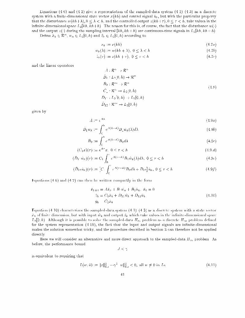
Equations (4.6) and (4.2) give a representation of the sampled-data system (4.1)�(4.3) as a discretesystem with a �nite-dimensional state vector x(kh) and control signal uk, but with the particular propertythat the disturbance w(kh+�); 0 � � < h, and the controlled output z(kh+� ); 0 � � < h, take values in thein�nite-dimensional space L2[kh; kh+h). The reason for this is, of course, the fact that the disturbance w(�)and the output z(�) during the sampling interval [kh; kh+h) are continuous-time signals in L2[kh; kh+h).
De�ne xk 2 Rn, wk 2 L2[0; h) and zk 2 L2[0; h) according to
xk := x(kh) (4:7a)
wk(�) := w(kh+ �); 0 � � < h (4:7b)
zk(� ) := z(kh + � ); 0 � � < h (4:7c)
and the linear operatorsA : Rn !Rn
B1 : L2[0; h)!Rn
B2 : Rm !Rn
C1 : Rn ! L2[0; h)
D11 : L2[0; h)! L2[0; h)
D12 : Rm ! L2[0; h)
(4:8)
given by
A := eAh (4:9a)
B1wk :=
Z h
0
eA(h��)
B1wk(�)d� (4:9b)
B2 :=
Z h
0
eA(h��)
B2d� (4:9c)
(C1x)(� ) := eA�x; 0 � � < h (4:9:d)
(D11wk)(� ) := C1
Z �
0
eA(���)
B1wk(�)d�; 0 � � < h (4:9e)
(D12uk)(� ) :=�C1
Z �
0
eA(���)
B2d�+D12
�uk; 0 � � < h (4:9f)
Equations (4.6) and (4.2) can then be written compactly in the form
xk+1 = Axk + B1wk + B2uk; x0 = 0
zk = C1xk + D11wk + D12uk (4:10)
yk = C2xk
Equation (4.10) characterizes the sampled-data system (4.1)�(4.3) as a discrete system with a state vectorxk of �nite dimension, but with input wk and output zk which take values in the in�nite-dimensional spaceL2[0; h). Although it is possible to solve the sampled-data H1 problem as a discrete H1 problem de�nedfor the system representation (4.10), the fact that the input and output signals are in�nite-dimensionalmakes the solution somewhat tricky, and the procedure described in Section 3 can therefore not be applieddirectly.
Here we will consider an alternative and more direct approach to the sampled-data H1 problem. Asbefore, the performance bound
J <
is equivalent to requiring that
L(w; u) := kzk2L2 � 2kwk2L2 < 0; all w 6= 0 in L2 (4:11)
41

holds. Now, by a completion of squares approach, the quadratic function L(w; u) can be expressed in aform analogous to (2.8) and (3.48). As the signal w is now a continuous-time signal, whereas the signal u isrestricted to change discontinuosly at the sampling instants fkhg according to Eq. (4.3), it follows that theassociated Riccati equation (corresponding to (2.7), or (3.47)) will be a mixed discrete/continuous Riccatiequation.
The direct Riccati-equation based approach leading to a mixed discrete/continuous Riccati equationwill not be used here, however. Instead of expanding (4.11) over the entire time interval as was done insections 2 and 3, we will here use an approach where the expansion is made separately for the individualsampling intervals. Note that (4.11) can be written
L(w; u) =
Z 1
0
(zT z � 2wTw)dt
=
1Xk=0
Z kh+h
kh
�zT (t)z(t) �
2wT (t)w(t)
�dt (4:12)
Consider the term
Lk(w; u) :=
Z kh+h
kh
�zT (t)z(t) �
2wT (t)w(t)
�dt (4:13)
which represents the contribution to L(w; u) from the sampling interval [kh; kh+h). We will now introducea completion of squares to expand the terms Lk(w; u) in a form similar to Eq. (2.8). The signals in (4.13)are given by the system equation (4.1) and the hold function (4.3), i.e.,
_x(t) = Ax(t) + B1w(t) + B2uk
z(t) = C1x(t) +D12uk; t 2 [kh; kh+ h)(4:14)
As u(t) is constant during the sampling interval, it may be included as part of the state vector. Hence(4.14) may be written in the form
�_x(t)
_u(t)
�=
�A B2
0 0
� �x(t)
u(t)
�+
�B1
0
�w(t);
�x(kh)
u(kh)
�=
�xk
uk
�
z(t) = [C1 D12 ]
�x(t)
u(t)
�; t 2 [kh; kh+ h)
or
_xe(t) = Aexe(t) +B1ew(t); xe(kh) =
�xk
uk
�z(t) = C1exe(t); t 2 [kh; kh+ h)
(4:15)
where
xe :=
�x
u
�
and
Ae :=
�A B2
0 0
�; B1e :=
�B1
0
�; C1e := [C1 D12 ] (4:16)
For (4.15) we obtain by a completion of squares argument a result analogous to (2.8). Introduce the Riccatidi�erential equation
� _P (t) = ATe P (t) + P (t)Ae +
�2P (t)B1eB
T1eP (t) + C
T1eC1e; P (h) = 0; t 2 [0; h] (4:17)
Assuming that Eq. (4.17) has a bounded positive semide�nite solution P (t) on [0; h], the quadratic functionLk(w; u) in Eq. (4.13) can be expressed as
42
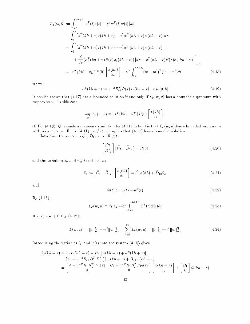
Lk(w; u) :=
Z kh+h
kh
�zT (t)z(t) �
2wT (t)w(t)
�dt
=
Z h
0
�zT (kh+ � )z(kh+ � ) �
2wT (kh+ � )w(kh+ � )
�d�
=
Z h
0
�zT (kh+ � )z(kh+ � ) �
2wT (kh+ � )w(kh+ � )
+d
d�
�xTe (kh+ � )P (� )xe(kh+ � )
��d� � x
Te (kh+ � )P (� )xe(kh+ � )
����h
�=0
= [xT (kh) uTk ]P (0)
�x(kh)
uk
��
2
Z kh+h
kh
(w � w0)T (w � w
0)dt (4:18)
wherew0(kh+ � ) :=
�2BTe1P (� )xe(kh+ � ); � 2 [0; h] (4:19)
It can be shown that (4.17) has a bounded solution if and only if Lk(w; u) has a bounded supremum withrespect to w. In this case,
supw
Lk(w; u) = [xT (kh) uTk ]P (0)
�x(kh)
uk
�;
cf. Eq. (4.18). Obviously a necessary condition for (4.11) to hold is that Lk(w; u) has a bounded supremumwith respect to w. Hence (4.11), or J < , implies that (4.17) has a bounded solution.
Introduce the matrices ~C1, ~D12 according to
�~CT1
~DT12
�[ ~C1
~D12 ] = P (0) (4:20)
and the variables ~zk and ~wk(t) de�ned as
~zk := [ ~C1~D12 ]
�x(kh)
uk
�= ~C1x(kh) + ~D12uk (4:21)
and~w(t) := w(t)� w
0(t) (4:22)
By (4.18),
Lk(w; u) = ~zTk ~zk � 2
Z kh+h
kh
~wT (t) ~w(t)dt (4:23)
Hence, also (cf. Eq. (4.12)),
L(w; u) := kzk2L2 � 2kwk2L2 =
1Xk=0
Lk(w; u) = k~zk2l2 � 2k ~wk2L2 (4:24)
Introducing the variables ~zk and ~w(t) into the system (4.15) gives
_xe(kh+ � ) = Aexe(kh+ � ) + Be1[ ~w(kh+ � ) +w0(kh+ � )]
= [Ae + �2Be1B
Te1P (� )]xe(kh+ � ) +Be1 ~w(kh+ � )
=
�A+
�2B1B
T1 P11(� ) B2 +
�2B1B
T1 P12(� )
0 0
� �x(kh+ � )
uk
�+
�B1
0
�~w(kh+ � )
43

where we have used (4.16) and introduced the partition
P :=
�P11 P12
PT12 P22
�(4:25)
in compliance with the partitions of Ae, Be1 and Ce1 in Eq. (4.17). From above, we have for the statevector x(kh+ � ),
_x(kh+� ) = [A+ �2B1BT1 P11(� )]x(kh+� )+[B2+
�2B1B
T1 P12(� )]uk+B1 ~w(kh+� ); � 2 [kh; kh+h) (4:26)
Denote the state transition matrix associated with the system matrix A + �2B1B
T1 P11(� ) in (4.26)
by �(�; �). Integrating (4.26) from kh to kh+ h gives
x(kh+ h) = �(h; 0)x(kh) +
Z h
0
�(h; �)[B2 + �2B1B
T1 P12(�)]d�uk +
Z h
0
�(h; �)B1 ~w(kh+ �)d� (4:27)
Combining (4.27), (4.21) and (4.2), we have that the sampled-data system (4.1)�(4.3) can be characterizedin the transformed variables ~z and ~w, (4.21) and (4.22), acording to the equations
xk+1 = ~Axk + ~B2uk +
Z h
0
�(h; �)B1 ~w(kh+ �)d�; x0 = 0
~zk = ~C1xk + ~D12uk (4:28)
yk = C2xk
where we have introduced xk := x(kh), and
~A := �(h; 0)
~B2 :=
Z h
0
�(h; �)[B2 + �2B1B
T1 P12(�)]d�
From the identity (4.24) it follows that J < holds for the sampled-data system (4.1)�(4.3) if and only if
~J := sup
� k~zkl2k ~wkL2
: ~w 6= 0; ~w 2 L2
�< (4:29)
holds for the system (4.28).Equation (4.28) gives a discrete representation of the sampled-data system (4.1)�(4.3). The represen-
tation (4.28) still involves the continuous-time signal ~w(t). However, the linear operator � : L2[0; h]!Rn
in (4.28),
�w :=
Z h
0
�(h; �)B1w(�)d� (4:30)
can be decomposed as (cf. Problem B.6)� = [ �� 0 ]
where �� has a matrix representation ~B1, which is de�ned by
~B1~BT1 := ����� = ��� =
Z h
0
�(h; �)B1BT1 �
T (h; �)d� (4:31)
Introducing the matrix representation ~B1 of the linear operator � into the system equations (4.28) resultsin the following theorem, which follows from the equivalence of J < and (4.29), and the fact that ~B1 isa matrix representation of the operator � in Eq. (4.30).
44

Theorem 4.1. Consider the sampled-data system (4.1)�(4.3). Let > 0 be given and assume that the
Riccati di�erential equation (4.17) has a bounded solution. De�ne the �nite-dimensional discrete system
xk+1 = ~Axk + ~B1~vk + ~B2uk; x0 = 0
~zk = ~C1xk + ~D12uk (4:32)
yk = C2xk
where
~A = �(h; 0);
~B1~BT1 =
Z h
0
�(h; �)B1BT1 �
T (h; �)d�;
~B2 :=
Z h
0
�(h; �)[B2 + �2B1B
T1 P12(�)]d�;�
~CT1
~DT12
�[ ~C1
~D12 ] := P (0);
�(�; �) is the state transition matrix associated with the system matrix A + �2B1B
T1 P11(� ), and P (�) is
the solution of the Riccati di�erential equation (4.17), partitioned as in (4.25).
Then for any discrete controller u = Ky the following statements are equivalent:
(i) K stabilizes the sampled-data system described by Eqs. (4.1)�(4.3) and achieves the performance bound
J < .
(ii) K stabilizes the discrete system (4.32) and achieves the performance bound
sup
�k~zkl2k~vkl2
: ~v 6= 0; ~v 2 l2
�< : (4:33)
Theorem 4.1 shows that the problem of �nding a discrete controller which achieves the performancebound J < for the sampled-data system (4.1)�(4.3) is equivalent to the problem of �nding a discretecontroller which achieves the performance bound (4.33) for the �nite-dimensional discrete system (4.32).This problem can be solved by the methods described in Section 3.
To conclude let's give explicit formulae for the system matrices in (4.32). De�ne the exponentialmatrix �
�11 �12
�21 �22
�(t) := exp
���
Ae �2Be1B
Te1
�CTe1Ce1 �AT
e
�t
�(4:34)
where Ae, Be1 and Ce1 are the matrices which appear in the Riccati equation (4.17), and are de�ned inEq. (4.16). From the structure of Ae and Be1 and the de�nition of the matrix exponential it follows that�11 and �12 can be partitioned according to
�11 =
��1111 �1112
0 I
�; �12 =
��1211 0
0 0
�(4:35)
The matrices in (4.32) can now be expressed in terms of the matrix exponential �(h) as follows
Lemma 4.1. The system matrices in (4.32) are given by
~A = �1111(h)�1;
~B1~BT1 = � 2 ~A�1211(h);
~B2 := � ~A�1112(h);�~CT1
~DT12
�[ ~C1
~D12 ] = �21(h)�11(h)�1:
(4:36)
45

Notes and references
Although the sampled-data H1 problem was introduced later than continuous-time and discrete-timeproblems, there is a quite extensive literature on the subject. One reason for this is the fact that there aremany alternative ways to solve the problem. There are also many variations of the standard setup whichhas been described here. One can for example consider more general hold functions, or the problem whenthe hold function can be chosen freely, and is part of the design. Similarly, one may include the selection ofthe sampling pre�lter as part of the design process. Moreover, there are dual-rate sampled-data problemswhere the sampler and the hold function operate at di�erent rates. Solutions to all these problems can befound in the literature.
The standard sampled-dataH1 control problem described by equations (4.1)�(4.3) and the worst-caseperformance measure (4.5) was �rst solved by the so-called lifting technique based on the discrete systemrepresentation (4.10) in Bamieh et al. (1991), Bamieh and Pearson (1992) and Toivonen (1992a). Game-theory type procedures based on the quadratic cost (4.11) were applied in Sun et al. (1991, 1992, 1993) andToivonen (1992b). The game-theory type methods are sampled-data analogues to the methods describedin sections 2 and 3, and, due to the hybrid discrete/continuous nature of sampled-data control systems,they lead to mixed discrete/continuous Riccati equations. The approach summarized in Theorem 4.1 andLemma 4.1 is taken from Toivonen (1993). For still some alternative procedures to solve the sampled-dataH1 problem, see Kabamba and Hara (1990, 1993) and Tadmor (1991, 1992).
PROBLEMS
4.1. De�ne the matrix exponential��11 �12
�21 �22
�(t) := exp
���
A �2BB
T
�CTC �AT
�t
�:
Show that the solution P (t) of the Riccati di�erential equation
� _P (t) = ATP (t) + P (t)A+
�2P (t)BBT
P (t) +CTC; P (h) = 0; t 2 [0; h]
can be expressed asP (t) = �21(h� t)�11(h � t)�1; t 2 [0; h]
and the Riccati di�erential equation has a bounded solution on [0; h] if and only if �11(h� t) is nonsingularon [0; h].
4.2. Prove Lemma 4.1.[ Hint: Study the system �
_p1_p2
�=
�Ae
�2Be1B
Te1
�CTe1Ce1 �AT
e
� �p1
p2
�;
use the fact that the associated transition matrix is a matrix exponential of the form considered in Problem4.1, and introduce the variable transformation�
r(t)
s(t)
�:=
�I 0
�P (t) I
� �p1(t)
p2(t)
�:
See Toivonen (1993). ]
4.3. Compute a sampled-data controller which minimizes the L2-induced norm from the disturbance w tothe output z for the system
_x =
�0 1
0 �0:1�x+
�1
1
�w +
�1
1
�u
z = [1 0 ]x
yk = [1 0 ]x(kh)
Study how the achievable performance depends on the sampling time h.
46
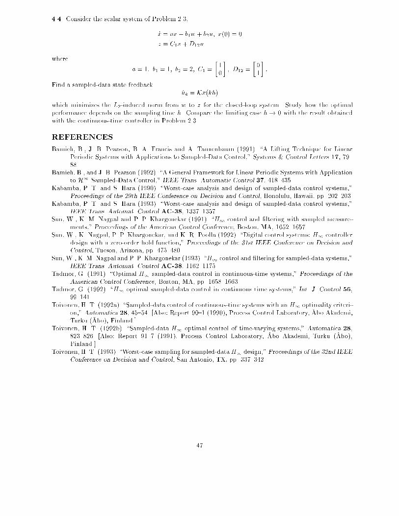
4.4. Consider the scalar system of Problem 2.3,
_x = ax+ b1w + b2u; x(0) = 0
z = C1x+D12u
where
a = 1; b1 = 1; b2 = 2; C1 =
�1
0
�; D12 =
�0
1
�:
Find a sampled-data state feedbackuk = Kx(kh)
which minimizes the L2-induced norm from w to z for the closed-loop system. Study how the optimalperformance depends on the sampling time h. Compare the limiting case h! 0 with the result obtainedwith the continuous-time controller in Problem 2.3.
REFERENCES
Bamieh, B., J. B. Pearson, B. A. Francis and A. Tannenbaum (1991). �A Lifting Technique for LinearPeriodic Systems with Applications to Sampled-Data Control,� Systems & Control Letters 17, 79�88.
Bamieh, B., and J. B. Pearson (1992). �A General Framework for Linear Periodic Systems with Applicationto H1 Sampled-Data Control,� IEEE Trans. Automatic Control 37, 418�435.
Kabamba, P. T. and S. Hara (1990). �Worst-case analysis and design of sampled-data control systems,�Proceedings of the 29th IEEE Conference on Decision and Control, Honolulu, Hawaii, pp. 202�203.
Kabamba, P. T. and S. Hara (1993). �Worst-case analysis and design of sampled-data control systems,�IEEE Trans. Automat. Control AC-38, 1337�1357.
Sun, W., K. M. Nagpal and P. P. Khargonekar (1991). �H1 control and �ltering with sampled measure-ments,� Proceedings of the American Control Conference, Boston, MA, 1652�1657.
Sun, W., K. Nagpal, P. P. Khargonekar, and K. R. Poolla (1992). �Digital control systems: H1 controllerdesign with a zero-order hold function,� Proceedings of the 31st IEEE Conference on Decision and
Control, Tucson, Arizona, pp. 475�480.Sun, W., K. M. Nagpal and P. P. Khargonekar (1993). �H1 control and �ltering for sampled-data systems,�
IEEE Trans. Automat. Control AC-38, 1162�1175.Tadmor, G. (1991). �Optimal H1 sampled-data control in continuous-time systems,� Proceedings of the
American Control Conference, Boston, MA, pp. 1658�1663.Tadmor, G. (1992). �H1 optimal sampled-data control in continuous time systems,� Int. J. Control 56,
99�141.Toivonen, H. T. (1992a). �Sampled-data control of continuous-time systems with an H1 optimality criteri-
on,� Automatica 28, 45�54. [Also: Report 90�1 (1990), Process Control Laboratory, Åbo Akademi,Turku (Åbo), Finland.]
Toivonen, H. T. (1992b). �Sampled-data H1 optimal control of time-varying systems,� Automatica 28,823�826. [Also: Report 91�7 (1991), Process Control Laboratory, Åbo Akademi, Turku (Åbo),Finland.]
Toivonen, H. T. (1993). �Worst-case sampling for sampled-dataH1 design,� Proceedings of the 32nd IEEEConference on Decision and Control, San Antonio, TX, pp. 337�342.
47

5. H1-OPTIMAL LOW-ORDER AND FIXED-STRUCTURE
CONTROLLERS
The synthesis procedures described above will in general result in controllers which have the same orderas the system, including all weighting �lters introduced for loop-shaping, etc. In practice the controllerorder may then be quite high, and it is therefore also well motivated to study procedures for designinglow-order controllers which achieve a speci�ed H1 performance bound. It can also be desirable to prescribea structure on the controller, such as, for example, a decentralized controller structure.
It turns out that the problem of designing low-order and �xed-structure controllers is signi�cantlyharder than the synthesis of optimal controllers without any constraints on order or structure. No closed-form solution of the low-orderH1 control problem exists. In fact, there is no procedure which can be provedto �nd the best low-order or �xed-structure control law. In spite of this, there are numerical proceduresfor constructing H1-optimal low-order and �xed-structure controllers which appear to work well. Theseprocedures fall into two main categories. The �rst class is based on a model reduction philosophy, whilethe second class of procedures is based on a more direct solution of the �xed-structure control problem.
(i) Methods based on model reduction techniques
- Perhaps the most straightforward approach to the design of low-order controllers is to start by con-structing a reduced-order model of the original system, followed by the design of an H1-optimalcontrol law for the reduced-order model using standard design methods. The resulting controller willhave the same order as the reduced-order model, and it is thus a low-order controller for the originalsystem. In this approach it is essential to perform the model reduction step in such a way that thecontroller designed for the reduced model will perform as well as possible when applied to the originalsystem.
- A dual approach to the one described above is to design a standard full-order H1-optimal controllerfor the the original system, followed by a reduction of the controller. Again, the crucial step in thisapproach is the controller reduction, which should be done in such a way that the reduced controllerperforms as well as possible. See for example Anderson and Liu (1989) and Mustafa and Glover (1991)for discussions of this approach.
(ii) Methods based on direct design of �xed-structure controllers
- A conceptually elegant approach to the low-orderH1 control problem is based on the parameterizationof all controllers of a given order which achieve a speci�ed H1 performance bound. The parameteri-zation can be expressed in terms of a pair of linear matrix inequalities (LMIs), together with a rankcondition. Unfortunately, the parameterization is in general not convex, and no algorithm exists whichis guaranteed to �nd a solution to the matrix equations, when such a solution exist. See Iwasaki andSkelton (1993) for a detailed description of this approach.
- Finally, one approach to the �xed-structure H1-optimal control problem is to characterize the pro-blem in terms of a parametric optimal control problem. This can be achieved by introducing anassociated auxiliary cost function, with the property that the solution to the H1 problem can befound by minimizing the associated cost function. The resulting minimization problem has the formof a parametric optimal control problem, and consists of �nding the optimal controller parameters tominimize a speci�ed cost function. Parametric optimal control problems have been studied extensivelyin the context of linear quadratic (LQ) control, and the same type of procedures applied there can beused to the parametric H1 control problem based on an auxiliary cost function. For various versionsof this approach, see DeShetler and Ridgely (1992) and Pensar and Toivonen (1993).
Note that of the above methods, only the parametric H1 control approach can be used to design�xed-structure controllers (such as decentralized control laws, etc.) other than low-order controllers, whilethe other methods are restricted to the design reduced-order control laws.
Numerical experience indicates that in many cases it is possible to achieve a closed-loop performancewhich is very close to the best performance which can be achieved with any controller, using quite simple
48

control laws. Therefore, the study of computational procedures for designing optimal low-order and �xed-structure controllers is well motivated from a practical point of view, although the problem does not havesuch a nice closed-form solution as the standard H1 control problem, when no constraints on the controllerorder or structure are imposed.
REFERENCES
Anderson, B. D. O., and Yi Liu (1989), �Controller Reduction: Concepts and Approaches,� IEEE Trans.
Automat. Control 34, 802�812.DeShetler, W. B., and D. B. Ridgely (1992), �Reduced Order H2 and H1 Compensation via Gradient
Techniques,� Proceedings of the 31st IEEE Conference on Decision and Control, Tucson, AZ, pp.2263�2267.
Iwasaki, T., and R. E. Skelton (1993), �All Low Order H1 Controllers with Covariance Upper Bound,�Proceedings of the 1993 American Control Conference, San Fransisco, CA, pp. 2180�2184.
Mustafa, D., and K. Glover (1991), �Controller Reduction by H1-Balanced Truncation,� IEEE Trans.
Automat. Control 36, 668�682.Pensar, J., and H. T. Toivonen (1993), �On the Design of Fixed-Structure H1 Optimal Controllers,�
Proceedings of the 32nd IEEE Conference on Decision and Control, San Antonio, TX, pp. 668�673.
49

6. MIXED H2/H1 CONTROL PROBLEMS
We have seen in Section 1 that the H1 control problem plays a central role in robustness considerations,whereas the H2 norm of the closed-loop system is important for control system performance. For example,in a stochastic framework the H2-norm represents the sum of the stationary variances of the outputvariables, cf. Section 1.4. In order to account for both closed loop robustness, as characterized by anH1-type performance bound, and control performance in terms of the H2 norm, mixed H2=H1 controlproblems have been introduced.
In order to introduce and motivate the mixedH2=H1 control problems, consider a plant with additiveuncertainty described by �
z0
y
�=�G0 +�W
� �w0
u
�(6:1)
where � is an uncertainty, such thatk�(i!)k � 1; all ! (6:2)
andW is a weighting �lter which determines the maximumuncertainty at various frequencies. The controlobjective could be to minimize the variances of the output z0 when w0 is a white noise disturbance, whileat the same time ensuring closed-loop stability in the face of the uncertainty �. The problem can beformulated as a mixed H2=H1 control problem as follows. The closed-loop control system can be writtenin the form shown in Fig. 6.1. (cf. Section 1.3). Here P is de�ned according to
"z1�z0
y
�#=
�0 W
I G0
� " w1�w0
u
�#(6:3)
From Section 1.3 we recall that the closed-loop system in Fig. 6.1 is stable for all � which satisfy (6.2) ifand only if kTz1w1k1 < 1, where Tz1w1 denotes the closed-loop transfer function from w1 to z1. The designproblem could then be characterized in terms of a mixed H2=H1 control problem as follows:
--
�
-
�
-
P
�
K
z0
z1
y
w0
w1
u
Fig. 6.1.
Find a controller which stabilizes the nominal plant G0 and minimizes the output variances obtained for
the nominal plant,
Ew0fzT0 z0g = kTz0w0k22 (with � = 0) (6:4a)
subject to the H1-norm bound
kTz1w1k1 < 1 (6:4b)
50

The problem in (6.4) de�nes an LQ problem with an H1-norm bound. The objective is to minimizethe LQ-cost kTz0w0k22 for the nominal plant G0 subject to the robust stability bound (6.4b), which ensuresclosed-loop stability for all uncertainties � which satisfy (6.2).
The problem in (6.4) does not take into account the fact that the uncertainty � a�ects the LQ-performance as well. The robust performance problem, which attempts to minimize the worst LQ-performancein the speci�ed uncertainty set, can be formulated as follows:
Find a controller which stabilizes the nominal plant G0, achieves the H1 norm bound (6.4b), and mini-
mizes the worst-case LQ cost
sup�
�kTz0w0k22 : k�(i!)k � 1; all !
�(6:5)
where Tz0w0 is determined for the interconnection in Fig. 6.1, and thus depends on �.
In practice, the best choice would probably be to minimize some realistic combination of nominal H2
performance (� = 0) and worst-case performance (6.5).As the above discussion shows there are many ways to combine H2 and H1 criteria. Mixed H2=H1
control is a collective term which has been used to refer to such problems. Here we shall only brie�ydescribe some of the main points involved in these problems.
To �x the ideas, we assume that the system is described by the state-space equation
_x = Ax+B0w0 +B1w1 + B2u
z0 = C0x+D02u
z1 = C1x+D12u
y = C2x+D20w0 +D21w1
(6:6)
The LQ problem with an H1-norm bound can be stated as follows (cf (6.4)):
Find a controller u = Ky which stabilizes the system (6.6) and minimizes
kTz0w0k22 (6:7a)
subject to
kTz1w1k1 < 1 (6:7b)
No closed-form solution to the general mixed H2=H1 problem in (6.7) is known. The only knownway to solve (6.7) is by �xing the controller structure, and by �nding the optimal controller parameters bydirect optimization. Assuming a linear controller u = Ky with state-space representation
_xc = Acxc + Bcy
u = Ccxc
(6:8)
the closed-loop (6.6), (6.8) becomes
�_x
_xc
�=
�A B2Cc
BcC2 Ac
� �x
xc
�+
�B0
BcD20
�w0
+
�B1
BcD21
�w1
z0 = [C0 D02Cc ]
�x
xc
�
z1 = [C1 D12Cc ]
�x
xc
�(6:9)
51

or, simply_xcl = Fxcl + G0w0 + G1w1
z0 = H0xcl
z1 = H1xcl
(6:10)
where xcl := [xT ; xTc ]T , and the matrices F , G0, G1, H0 and H1, which are functions of the controller
parameters in (6.8), are de�ned in accordance with (6.9).The H2-norm in (6.7a) is given by (cf. Section 1.4)
kTz0w0k22 = tr(GT0XG0) (6:11)
where X is the positive semide�nite solution to the matrix Lyapunov equation
FTX +XF +H
T0 H0 = 0 (6:12)
The H1-norm constraint in (6.7b) can also be expressed in terms of a matrix equation; we have from theH1 theory presented in Section 2 that kTz1w1k1 < 1 if and only if there exists a positive semide�nitematrix Y which satis�es the Riccati equation
FTY + Y F + Y G1G
T1 Y +H
T1 H1 = 0 (6:13a)
and such thatF + G1G
T1 Y is stable (6:13b)
See Remark 2.1 and Theorem 2.2. The problem of �nding a controller (6.8) which minimizes the LQ cost(6.11) subject to the H1 norm bound (6.13) must today be solved by optimization-based approaches.
There are, however, some special situations where more is known about the solution. An importantexample is the case when the outputs are the same, i.e., z0 = z1 (or the dual problem, where the inputs arethe same; w0 = w1), and an upper bound for the the LQ cost is minimized. In the case when the outputsare the same, H0 = H1, and Eq. (6.13a) becomes
FTY + Y F + Y G1G
T1 Y +H
T0 H0 = 0 (6:14)
which di�ers from (6.12) only in the symmetric positive semide�nite term Y G1GT1 Y . From standard
properties of matrix Lyapunov equations we have that, if F is a stable matrix, and Q1 and Q2 are symmetricpositive semide�nite matrices such thatQ2 � Q1 (i.e.,Q2�Q1 � 0, positive semide�nite), then the solutionsof
FTP1 + P1F + Q1 = 0
FTP2 + P2F + Q2 = 0
satisfy P2 � P1. Hence, (6.12) and (6.14) imply Y � X, and it follows that
kTz0w0k22 = tr(GT0XG0) � tr(GT
0 Y G0) (6:15)
providing an upper bound for the LQ cost. The following problem is then de�ned:
Consider the closed-loop system (6.10) with H0 = H1. Find a controller (6.8) which minimizes
tr(GT0 Y G0) (6:16)
where Y is given by (6.13).
Although problem (6.16) appears somewhat contrived, it is interesting due to the fact that the structureof its solution is known. Firstly, it is known that the optimal controller has the same order as the system.In this respect problem (6.16) is thus similar to the standard LQ and H1 control problems. Secondly,necessary and su�cient optimality conditions for the problem (6.16) been derived.
52

Notes and references
The concept of combining LQ and H1 performance objectives appears to be due to Bernstein and Haddad(1989), who introduced a dual version of problem (6.16) (with w0 = w1), and studied its solution. Necessaryand su�cient optimality conditions for problem (6.16) have been given, for example by Doyle et al. (1989,1994) and Zhou et al. (1990). Although necessary and su�cient optimality conditions of problem (6.16) andits dual are known, their solution is commonly regarded to be numerically quite demanding. Khargonekarand Rotea (1991) have in an important paper presented a convex optimization approach to the Bernstein-Haddad problem, for which convergence to the optimum can be proven. See also Yeh et al. (1992) for adiscussion of the connection between problem (6.16) and its dual.
For the general mixed H2=H1 control problem in (6.7) it does not seem possible to �nd so nicesolutions, and this problem has therefore not attracted so much attention in the control literature. Variouscomputational approaches based on parametric optimal control type methods have been applied to thisproblem, see Ridgley et al. (1992a, 1992b) and Pensar and Toivonen (1994).
The worst-case performance minimization problem (6.5) is still unsolved. One step toward its solutionis the work of Stoorvogel (1993), who studies the problem in the case when the uncertainty � belongs tothe larger class of nonlinear, and possibly noncausal, bounded operators. Interestingly, it turns out thatproblem (6.16) plays an important in the solution of the worst-case performance minimization problem.
REFERENCES
Bernstein, D. S., and W. M. Haddad (1989), �LQG Control with an H1 Performance Bound: A RiccatiEquation Approach,� IEEE Trans. Automat. Control 34, 293�305.
Doyle, J., K. Zhou, and B. Bodenheimer (1989), �Optimal Control with Mixed H2 and H1 PerformanceObjectives,� Proceedings of the 1989 American Control Conference, Pittsburgh, PA, pp. 2065�2070.
Doyle, J., K. Zhou, K. Glover, and B. Bodenheimer (1989), �Mixed H2 and H1 Performance ObjectivesII: Optimal Control,� IEEE Trans. Automat. Control 39, 1575�1587.
Pensar, J., and H. T. Toivonen (1994), �A Multimodel Mixed H2=H1 Problem for Plants with StructuredUncertainty,� IFAC Symposium ADCHEM'94, Kyoto, 1994.
Ridgley, D. B., L. Valavani, M. Dahleh, and G. Stein (1992a), �Solutions to the General Mixed H2=H1
Control Problem � Necessary Conditions for Optimality,�Proceedings of the 1992 American Control
Conference, Chicago, IL, pp. 1348�1352.Ridgley, D. B., C. P. Mracek, and L. Valavani (1992b), �Numerical Solutions to the General Mixed H2=H1
Optimization Problem,� Proceedings of the 1992 American Control Conference, Chicago, IL, pp.1353�1357.
Stoorvogel, A. A. (1993), �The RobustH2 Control Problem: AWorst-Case Design,� IEEE Trans. Automat.
Control 38, 1358�1370.Yeh, Hsi-Han, S. S. Banda, and B.-C. Chang (1992), �Necessary and Su�cient Conditions for Mixed H2
and H1 Optimal Control,� IEEE Trans. Automat. Control 37, 355�358.Zhou, K., J. Doyle, K. Glover, and B. Bodenheimer (1990), �Mixed H2 and H1 Control,� Proceedings of
the 1990 American Control Conference, San Diego, CA, pp. 2502�2507.
53
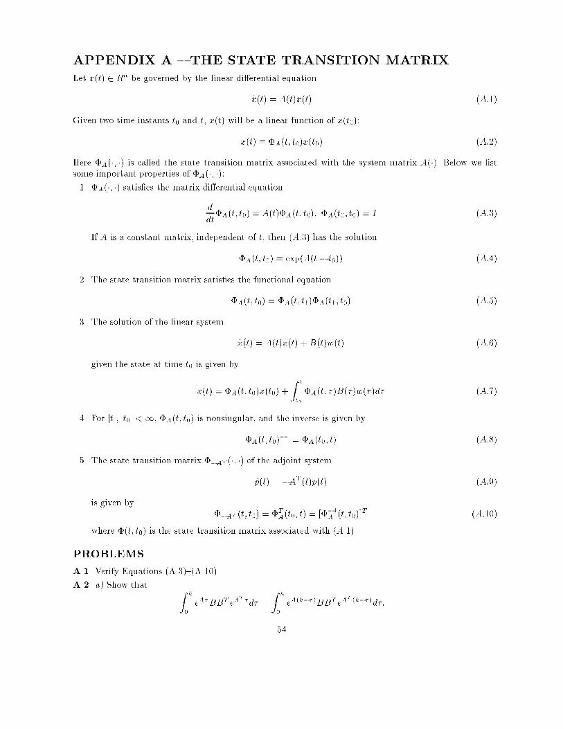
APPENDIX A � THE STATE TRANSITION MATRIX
Let x(t) 2 Rn be governed by the linear di�erential equation
_x(t) = A(t)x(t) (A:1)
Given two time instants t0 and t, x(t) will be a linear function of x(t0):
x(t) = �A(t; t0)x(t0) (A:2)
Here �A(�; �) is called the state transition matrix associated with the system matrix A(�). Below we listsome important properties of �A(�; �):1. �A(�; �) satis�es the matrix di�erential equation
d
dt�A(t; t0) = A(t)�A(t; t0); �A(t0; t0) = I (A:3)
If A is a constant matrix, independent of t, then (A:3) has the solution
�A(t; t0) = exp(A(t� t0)) (A:4)
2. The state transition matrix satis�es the functional equation
�A(t; t0) = �A(t; t1)�A(t1; t0) (A:5)
3. The solution of the linear system
_x(t) = A(t)x(t) +B(t)w(t) (A:6)
given the state at time t0 is given by
x(t) = �A(t; t0)x(t0) +
Z t
t0
�A(t; � )B(� )w(� )d� (A:7)
4. For jtj; jt0j <1, �A(t; t0) is nonsingular, and the inverse is given by
�A(t; t0)�1 = �A(t0; t) (A:8)
5. The state transition matrix ��AT (�; �) of the adjoint system
_p(t) = �AT (t)p(t) (A:9)
is given by��AT (t; t0) = �T
A(t0; t) = [��1A (t; t0)]T (A:10)
where �(t; t0) is the state transition matrix associated with (A:1).
PROBLEMS
A.1. Verify Equations (A.3)�(A.10).
A.2. a) Show that Z h
0
eA�BB
TeAT �
d� =
Z h
0
eA(h��)
BBTeAT (h��)
d�:
54

b) Show that
exp
��A BB
T
0 �AT
�h
�=
�eAh W (0; h)e�A
T h
0 e�AT h
�
where
W (0; h) :=
Z h
0
eA�BB
TeAT �
d�:
APPENDIX B � ADJOINT OPERATORS
In this appendix we review some basic properties of inner product spaces needed in Section 2.2.The L2-spaces introduced in Section 1.1 are equipped with an inner product (or scalar product), which
is denoted(x; y)
and is de�ned for any x; y 2 L2. For example, in L2[0;1) the inner product is de�ned as
(v; w) :=
Z 1
0
vT (t)w(t)dt; v; w 2 L2[0;1) (B:1)
and in L2(iR) we have
(v; w) :=1
2�
Z 1
�1
v�(i!)w(i!)d!; v; w 2 L2(iR) (B:2)
Note that the norms (1.1) and (1.3) are induced by the respective inner products in the sense that
kwk2 = (w;w)1=2; w 2 L2[0;1) (B:3a)
andkwk2 = (w; w)1=2; w 2 L2(iR) (B:3b)
A linear space X equipped with an inner product is called an inner product space. An inner product spacewhich is complete, i.e., it has the property that every Cauchy sequence in X converges in X, is called aHilbert space. The L2-spaces are Hilbert spaces.
Example B.1.
In Rn, we can de�ne the inner product
(y; x) := yTx; x; y 2 Rn
:
The corresponding norm iskxk = (x; x)1=2 = (xTx)1=2;
i.e. the Euclidian norm.
Next consider a linear operator T : X ! Y , where X and Y are inner product spaces. Then for x 2 X,u = Tx is in Y , and it makes sense to consider the following inner product in Y ,
(y; u) = (y; Tx)
where y 2 Y . Now it turns out that every linear operator T : X ! Y has associated with it an adjoint
operator T � : Y ! X, which has the property that for all x 2 X, y 2 Y ,
(y; Tx)Y = (T �y; x)X (B:4)
55

holds, where (�; �)Y denotes the inner product de�ned on Y , and analogously for (�; �)X.Example B.2.
Let T : Rn !Rm. Then T has a representation in terms of an m � n-matrix, whose elements are de�nedin terms of the action of T on the unit vectors in Rn. With some abuse of notation, denote the matrixrepresentation of T by T as well. With the de�nition of inner product in Example B.1, we have for anyx 2 Rn, y 2 Rm,
(y; Tx)Rm = yTTx = (TT
y)Tx = (TTy; x)Rn =: (T �y; x)Rn
and it follows that T � = TT , the matrix transpose.
Example B.3.
In L2(iR), de�ne the linear operator G : L2(iR)! L2(iR) de�ned so that
v = Gw
is given byv(i!) := (Gw)(i!) = G(i!)w(i!):
where G(�) is a transfer function matrix. Then, for u; w in L2(iR),
(u;Gw) = 1
2�
Z 1
�1
u�(i!)G(i!)w(i!)d!
=1
2�
Z 1
�1
�G�(i!)u(i!)
��w(i!)d!
= (G�u; w):
Hence the adjoint operator G� : L2(iR)! L2(iR) is de�ned so that y = G�u is given by
y(i!) = (G�u)(i!) = G�(i!)u(i!) = G
T (�i!)u(i!)
In particular, if the operator G has the state-space representation (A;B;C;D), i.e.,
G(i!) = C(i!I � A)�1B +D;
then G� has the state-space representation (�AT; C
T;�BT
; DT ), because
G�(i!) = B
T (�i!I � AT )�1CT +D
T
= �BT (i!I + AT )�1CT +D
T
Example B.4
Consider the linear operator G : L2[0; T ]! L2[0; T ] de�ned so that
y = Gw
is given by the state-space equations
_x(t) = Ax(t) + Bw(t); x(0) = 0
y(t) = Cx(t) +Dw(t); t 2 [0; T ]
We shall determine the adjoint operator G�. Now (cf. (A.7))
y(t) = Cx(t) +Dw(t) = C
Z t
0
�A(t; � )Bw(� )d� +Dw(t)
56

and for any z 2 L2[0; T ], we can form the inner product in L2[; 0; T ], giving
(z;Gw) =Z T
0
zT (t)
�C
Z t
0
�A(t; � )Bw(� )d� +Dw(t)�dt
=
Z T
t=0
Z t
�=0
zT (t)C�A(t; � )Bw(� )d�dt+
Z T
0
zT (t)Dw(t)dt
=
Z T
�=0
Z T
t=�
zT (t)C�A(t; � )Bw(� )dtd� +
Z T
0
zT (t)Dw(t)dt
=
Z T
�=0
�Z T
t=�
BT�T
A(t; � )CTz(t)dt
�Tw(� )d� +
Z T
0
[DTz(� )]Tw(� )d�
=
Z T
�=0
�Z T
t=�
BT�T
A(t; � )CTz(t)dt+D
Tz(� )
�Tw(� )d�
=: (G�z; w);
where G�z has been de�ned accoording to
(G�z)(� ) =Z T
�
BT�T
A(t; � )CTz(t)dt+D
Tz(� )
But in Appendix A we saw that the state transition matrix ��AT (t; t0) associated with the system matrix�AT is ��AT (t; t0) = �T
A(t0; t). Introducing ��AT (�; �) into the above expression gives
(G�z)(� ) =Z T
�
BT��AT (�; t)C
Tz(t)dt+D
Tz(� )
= �Z �
T
BT��AT (�; t)C
Tz(t)dt+D
Tz(� )
Comparing this expression with (A:7) and using the de�nition of ��AT (�; �) shows that the adjoint operatorG� can be represented in state-space form as
(G�z)(� ) = s(� );
where_p = �AT
p� CTz; p(T ) = 0
s = BTp +D
Tz
or,� _p = A
Tp+ C
Tz; p(T ) = 0
s = BTp+D
Tz
The norm of the adjoint operator
Consider the operator T : X ! Y , where X and Y are Hilbert spaces. The operator norm induced by thenorms k � kX and k � kY in X and Y is de�ned as
kTk := sup
�kTxkYkxkX : x 2 X; x 6= 0
�(B:5)
For the adjoint operator T � : Y ! X, we have anologously,
kT �k := sup
�kT �ykXkykY : y 2 Y; y 6= 0
�(B:6)
57

It can be shown that for a bounded linear operator the norm of the adjoint operator and the norm of theoperator itself are equal,
kT �k = kTk (B:7)
Example B.5
Consider the operator T : Rn !Rm in Example B.2. Then
kTk = sup
�kTxkkxk : x 2 Rn
; x 6= 0
�
= sup��xTTT
Tx
xTx
�1=2: x 2 Rn
; x 6= 0
�= ��(T )
where ��(T ) denotes the maximum singular value of T . But the transpose TT has the same singular valuesas T , so that ��(T ) = ��(TT ), and hence
kTk = ��(T ) = ��(TT ) = kTTk = kT �k
Thus we have shown (B:7) for matrix operator.
Example B.6
Consider the linear operator G : L2(iR) ! L2(iR) in Example B.3. From equations (1.8) and (1.9) werecall that
kGk = kGk1 := sup!
��(G(i!))
Hence
kG�k = kG�k1 := sup!
��(G�(i!))
= sup!
��(G(i!))
= kGk1= kGk
Finally, let's note the following relations which hold for adjoint operators and which are easy to verify:
(G1 + G2)� = G�1 + G�2 (B:8)
and(G1G2)� = G�2G�1
PROBLEMS
B.1. Make a literature study to clarify the following concepts:- metric space,- linear space,- normed linear space,- Banach space.Give speci�c examples of all the spaces. Give also an example of a normed linear space which is not a
Banach space.
B.2. Make a literature study to clarify the following concepts:- inner product space,- Hilbert space.
58
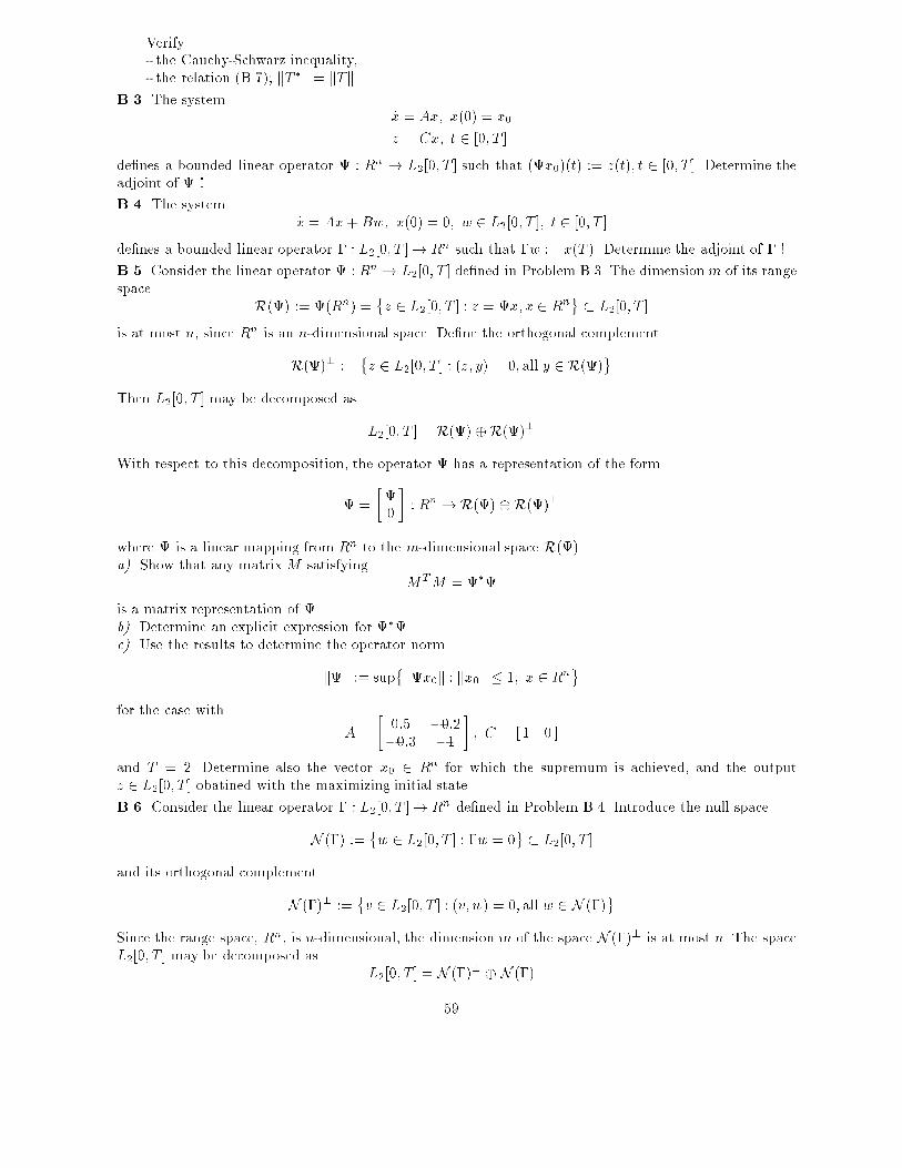
Verify- the Cauchy-Schwarz inequality,- the relation (B.7); kT �k = kTk.
B.3. The system_x = Ax; x(0) = x0
z = Cx; t 2 [0; T ]
de�nes a bounded linear operator : Rn ! L2[0; T ] such that (x0)(t) := z(t); t 2 [0; T ]. Determine theadjoint of !
B.4. The system_x = Ax+ Bw; x(0) = 0; w 2 L2[0; T ]; t 2 [0; T ]
de�nes a bounded linear operator � : L2[0; T ]! Rn such that �w := x(T ). Determine the adjoint of � !
B.5. Consider the linear operator : Rn ! L2[0; T ] de�ned in Problem B.3. The dimensionm of its rangespace
R() := (Rn) =�z 2 L2[0; T ] : z = x; x 2 R
n � L2[0; T ]
is at most n, since Rn is an n-dimensional space. De�ne the orthogonal complement
R()? :=�z 2 L2[0; T ] : (z; y) = 0; all y 2 R()
Then L2[0; T ] may be decomposed as
L2[0; T ] = R() �R()?
With respect to this decomposition, the operator has a representation of the form
=
��
0
�: Rn !R() �R()?
where � is a linear mapping from Rn to the m-dimensional space R().
a) Show that any matrix M satisfyingM
TM = �
is a matrix representation of �.b) Determine an explicit expression for �.c) Use the results to determine the operator norm
kk := sup�kx0k : kx0k � 1; x 2 R
n
for the case with
A =
�0:5 �0:2�0:3 �1
�; C = [1 0 ]
and T = 2. Determine also the vector x0 2 Rn for which the supremum is achieved, and the output
z 2 L2[0; T ] obatined with the maximizing initial state.
B.6. Consider the linear operator � : L2[0; T ]! Rn de�ned in Problem B.4. Introduce the null space
N (�) :=�w 2 L2[0; T ] : �w = 0
� L2[0; T ]
and its orthogonal complement
N (�)? :=�v 2 L2[0; T ] : (v; w) = 0; all w 2 N (�)
Since the range space, Rn, is n-dimensional, the dimension m of the space N (�)? is at most n. The spaceL2[0; T ] may be decomposed as
L2[0; T ] = N (�)? � N (�)
59
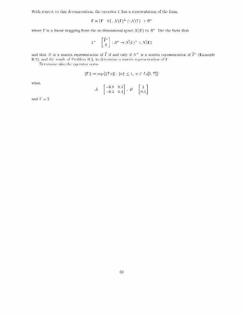
With respect to this decomposition, the operator � has a representation of the form
� = [ �� 0 ] : N (�)? �N (�)! Rn
where �� is a linear mapping from the m-dimensional space N (�) to Rn. Use the facts that
�� =
����
0
�: Rn !N (�)? � N (�)
and that N is a matrix representation of �� if and only if NT is a matrix representation of ��� (ExampleB.2), and the result of Problem B.5, to determine a matrix representation of �.
Determine also the operator norm
k�k := sup�k�wk : kwk � 1; w 2 L2[0; T ]
when
A =
��0:8 0:3
�0:5 0:4
�; B =
�1
0:5
�
and T = 2.
60