A Higher-Order Unstructured Finite Volume Solver forThree-Dimensional Compressible Flows

Shayan Hoshyari

a thesis submitted in partial fulfillmentof the reqirements for the degree of

Master of Applied Sciencein

Mechanical Engineeringat

The University of British Columbia

August 2017

Abstract

High-order accurate numerical discretization methods are attractive for their potential to signicantlyreduce the computational costs compared to the traditional second-order methods. Among the variousunstructured higher-order discretization schemes, the k-exact reconstruction nite volume method isof interest for its straightforward mathematical formulation, and its compatibility with the currentlower-order industrial solvers. However, current three-dimensional nite volume solvers are limitedto the solution of inviscid and laminar viscous ow problems. Since three-dimensional turbulent owsappear in many industrial applications, the current thesis takes the rst step towards the developmentof a three-dimensional higher-order nite volume solver for the solution of both inviscid and viscousturbulent steady-state ow problems.

The k-exact nite volume formulation of the governing equations is rederived in a dimension-independentmanner, where the negative Spalart-Allmaras turbulence model is employed. This one-equation modelis reasonably accurate for many ow conditions, and its simplicity makes it a good starting point forthe development of numerical algorithms. Then, the three-dimensional mesh preprocessing steps fora nite volume simulation are presented, including higher-order accurate numerical quadrature, andcapturing the boundary curvature in highly anisotropic meshes. Also, the issues of k-exact reconstruc-tion in handling highly anisotropic meshes are reviewed and addressed.

Since three-dimensional problems can require much more memory than their two-dimensional coun-terparts, solution methods that work in two dimensions might not be feasible in three dimensionsanymore. As an attempt to overcome this issue, a practical and parallel scalable method for the solu-tion of the discretized system of nonlinear equations is presented.

Finally, the solution of four three-dimensional test problems are studied: Poisson’s equation in a cubicdomain, inviscid ow over a sphere, turbulent ow over a at plate, and turbulent ow over an ex-truded NACA 0012 airfoil. The solution is veried, and the resource consumption of the ow solveris measured. The results demonstrate the benet and practicality of using higher-order methods forobtaining a certain level of accuracy.

i

Lay Summary

The nite volume method is a popular numerical scheme for the solution of aerodynamic ow prob-lems. Although conventional nite volume schemes are mostly second-order accurate, there has beena growing interest in higher-order accurate numerical methods, since they can be considerably moreecient in terms of computational resources for achieving a certain level of accuracy.

Higher-order nite volume methods have been successfully developed for a wide range of two-dimensionalow problems. Nevertheless, numerical methods that work in two dimensions might not be feasiblein three dimensions anymore, since three-dimensional problems can require much more memory thantheir two-dimensional counterparts. The current thesis aims at identifying, and resolving such short-comings to construct a working three-dimensional nite volume solver with an emphasis on turbulentows. Subsequently, three-dimensional benchmark ow problems are solved to verify and assess theperformance of the developed numerical method.

ii

Preface

All the work presented in this thesis is an intellectual product of a working relationship betweenShayan Hoshyari and Dr. Carl Ollivier-Gooch. The implementation of the methods, the data analysis,and the manuscript preparations were done by Shayan Hoshyari with invaluable guidance from CarlOllivier-Gooch throughout the process.

iii

Contents

Abstract i

Lay Summary ii

Preface iii

List of Tables vi

List of Figures vii

List of Symbols viii

Acknowledgments xii

1 Introduction 11.1 Motivation . . . . . . . . . . . . . . . . . . . . . . . . . . . . . . . . . . . . . . . . . . . 11.2 Objectives . . . . . . . . . . . . . . . . . . . . . . . . . . . . . . . . . . . . . . . . . . . 31.3 Thesis Outline . . . . . . . . . . . . . . . . . . . . . . . . . . . . . . . . . . . . . . . . . 3

2 Background 52.1 The Finite Volume Method . . . . . . . . . . . . . . . . . . . . . . . . . . . . . . . . . . 52.2 K-exact Reconstruction . . . . . . . . . . . . . . . . . . . . . . . . . . . . . . . . . . . . 62.3 Studied Equations . . . . . . . . . . . . . . . . . . . . . . . . . . . . . . . . . . . . . . . 9

2.3.1 Poisson’s Equation . . . . . . . . . . . . . . . . . . . . . . . . . . . . . . . . . . 92.3.2 Navier-Stokes Equations . . . . . . . . . . . . . . . . . . . . . . . . . . . . . . . 102.3.3 Extension to Turbulent Flows . . . . . . . . . . . . . . . . . . . . . . . . . . . . 11

2.4 Numerical Flux Functions . . . . . . . . . . . . . . . . . . . . . . . . . . . . . . . . . . . 132.4.1 Inviscid Flux . . . . . . . . . . . . . . . . . . . . . . . . . . . . . . . . . . . . . . 132.4.2 Viscous Flux . . . . . . . . . . . . . . . . . . . . . . . . . . . . . . . . . . . . . . 15

3 Three-Dimensional Mesh Processing 173.1 Element Mapping and Quadrature . . . . . . . . . . . . . . . . . . . . . . . . . . . . . . 173.2 Creating Curved Anisotropic Meshes . . . . . . . . . . . . . . . . . . . . . . . . . . . . 203.3 Modied Basis Functions for Highly Anisotropic Meshes . . . . . . . . . . . . . . . . . 24

4 Solving the Discretized System of Equations 284.1 Pseudo Transient Continuation . . . . . . . . . . . . . . . . . . . . . . . . . . . . . . . 284.2 Linear Solvers . . . . . . . . . . . . . . . . . . . . . . . . . . . . . . . . . . . . . . . . . 30

iv

4.3 Preconditioning . . . . . . . . . . . . . . . . . . . . . . . . . . . . . . . . . . . . . . . . 304.3.1 Point Gauss-Seidel . . . . . . . . . . . . . . . . . . . . . . . . . . . . . . . . . . 314.3.2 Block Jacobi . . . . . . . . . . . . . . . . . . . . . . . . . . . . . . . . . . . . . . 334.3.3 ILU . . . . . . . . . . . . . . . . . . . . . . . . . . . . . . . . . . . . . . . . . . . 34

4.4 Improved Preconditioning Algorithms . . . . . . . . . . . . . . . . . . . . . . . . . . . . 344.4.1 Inner GMRES Iterations . . . . . . . . . . . . . . . . . . . . . . . . . . . . . . . 354.4.2 Lines of Strong Coupling Between Unknowns . . . . . . . . . . . . . . . . . . . 35

4.5 Numerical Comparisons . . . . . . . . . . . . . . . . . . . . . . . . . . . . . . . . . . . 37

5 Three-Dimensional Results 425.1 Poisson’s Equation in a Cubic Domain . . . . . . . . . . . . . . . . . . . . . . . . . . . . 425.2 Inviscid Flow Around a Sphere . . . . . . . . . . . . . . . . . . . . . . . . . . . . . . . . 435.3 Turbulent Flow Over a Flat Plate . . . . . . . . . . . . . . . . . . . . . . . . . . . . . . . 495.4 Turbulent Flow Over an Extruded Airfoil . . . . . . . . . . . . . . . . . . . . . . . . . . 53

6 Conclusions 58

Bibliography 61

A ANSLib Command-Line Options 67A.1 Two-Dimensional Turbulent Flow over a NACA 0012 Airfoil from Section 4.5 . . . . . 67A.2 Poisson’s Equation from Section 5.1 . . . . . . . . . . . . . . . . . . . . . . . . . . . . . 69A.3 Inviscid Flow Over a Sphere from Section 5.2 . . . . . . . . . . . . . . . . . . . . . . . . 70A.4 Turbulent Flow Over a Flat Plate from Section 5.3 . . . . . . . . . . . . . . . . . . . . . 71A.5 Turbulent Flow Over an Extruded NACA 0012 Airfoil from Section 5.4 . . . . . . . . . 72

B Sample Script for Running a Parallel Job on Grex 74

v

List of Tables

2.1 Dimensionless empirical parameters used in the negative S-A model . . . . . . . . . . . 12

3.1 Performance of the linear elasticity solver . . . . . . . . . . . . . . . . . . . . . . . . . . 24

4.1 Preconditioning methods considered . . . . . . . . . . . . . . . . . . . . . . . . . . . . 394.2 Performance comparison for dierent preconditioning schemes . . . . . . . . . . . . . 414.3 Computed drag and lift coecients for the NACA 0012 airfoil . . . . . . . . . . . . . . 41

5.1 Number of iterations and the resource consumption of the ow solver for the sphereproblem . . . . . . . . . . . . . . . . . . . . . . . . . . . . . . . . . . . . . . . . . . . . . 48

5.2 Computed value and convergence order of the drag coecient and the skin frictioncoecient at the point x = (0.97,0,0.5) for the at plate problem . . . . . . . . . . . . 52

5.3 Number of iterations and the resource consumption of the ow solver for the at plateproblem . . . . . . . . . . . . . . . . . . . . . . . . . . . . . . . . . . . . . . . . . . . . . 53

5.4 Computed drag and lift coecients for the extruded NACA 0012 airfoil problem . . . . 565.5 Resource consumption of the ow solver for the extruded NACA 0012 problem . . . . . 57

vi

List of Figures

2.1 Illustration of terminology in nite volume discretization . . . . . . . . . . . . . . . . . 62.2 Reconstruction stencils for a control volume . . . . . . . . . . . . . . . . . . . . . . . . 9

3.1 Control volumes for cell-centered and cell-vertex methods . . . . . . . . . . . . . . . . 183.2 First order reference Lagrange elements . . . . . . . . . . . . . . . . . . . . . . . . . . . 193.3 Geometry of the curved mesh generation test case . . . . . . . . . . . . . . . . . . . . . 233.4 Curved mesh displacement magnitude . . . . . . . . . . . . . . . . . . . . . . . . . . . 243.5 Residual per iteration for the linear elasticity solver . . . . . . . . . . . . . . . . . . . . 253.6 Construction of approximate wall coordinates for a two-dimensional control volume . 26

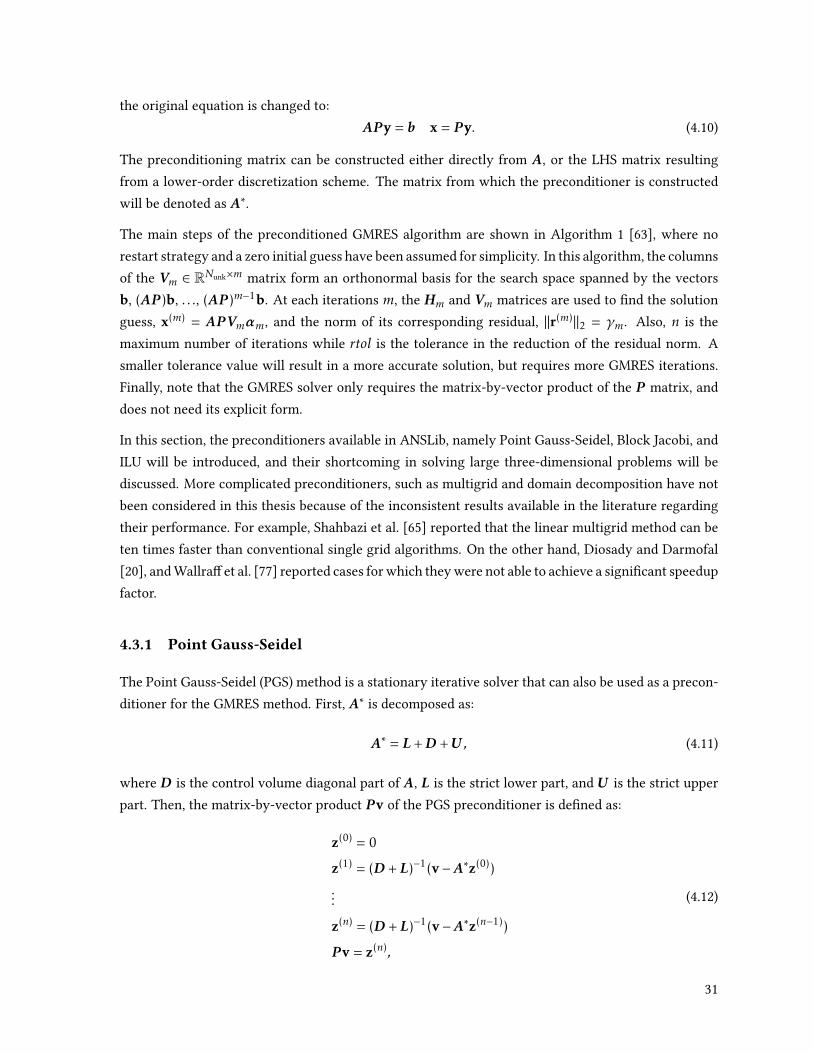
4.1 Schematic of Block Jacobi decomposition . . . . . . . . . . . . . . . . . . . . . . . . . . 334.2 Mesh and lines of strong unknown coupling for the geometry of a NACA 0012 airfoil . 384.3 Comparison of residual histories for the NACA 0012 problem obtained using dierent

preconditioning algorithms . . . . . . . . . . . . . . . . . . . . . . . . . . . . . . . . . . 394.4 Residual history for the NACA 0012 problem on the nest mesh of 400K control volumes 40

5.1 Exact solution of Poisson’s problem . . . . . . . . . . . . . . . . . . . . . . . . . . . . . 435.2 Dierent meshes for the solution of Poisson’s problem . . . . . . . . . . . . . . . . . . 445.3 Discretization error versus mesh size for Poisson’s problem . . . . . . . . . . . . . . . . 455.4 Symmetric cut of the coarsest mesh near the sphere surface . . . . . . . . . . . . . . . 455.5 Relative entropy norm versus mesh size for the sphere problem . . . . . . . . . . . . . 465.6 Computed Mach contours on the x3 = 0 symmetry plane for the sphere problem . . . . 475.7 Norm of the residual vector per PTC iteration for the sphere problem . . . . . . . . . . 485.8 The parallel speedup of the solver for the sphere problem . . . . . . . . . . . . . . . . . 495.9 Coarsest mesh for the at plate problem. . . . . . . . . . . . . . . . . . . . . . . . . . . 505.10 Distribution of the turbulence working variable on the plane x3 = 0.5 for the at plate

problem . . . . . . . . . . . . . . . . . . . . . . . . . . . . . . . . . . . . . . . . . . . . . 515.11 Distribution of the nondimensional eddy viscosity on the line (x1 = 0.97)∧ (x3 = 0.5)

for the at plate problem . . . . . . . . . . . . . . . . . . . . . . . . . . . . . . . . . . . 515.12 Norm of the residual vector per PTC iteration for the at plate problem . . . . . . . . . 525.13 The parallel speedup of the solver for the at plate problem . . . . . . . . . . . . . . . . 535.14 Meshes for the extruded NACA 0012 problem . . . . . . . . . . . . . . . . . . . . . . . 545.15 Distribution of the turbulence working variable for the extruded NACA 0012 problem

on the x3 = 0 plane . . . . . . . . . . . . . . . . . . . . . . . . . . . . . . . . . . . . . . 555.16 Distribution of surface pressure coecient on the intersection of the extruded NACA

0012 airfoil and the x3 = 0.5 plane. . . . . . . . . . . . . . . . . . . . . . . . . . . . . . 565.17 Norm of the residual vector per PTC iteration for the extruded airfoil problem . . . . . 57

vii

List of Symbols

Orders

k Order of reconstruction

l Order of Lagrangian polynomials

p Order of nite element basis functions

q Order of accuracy for a quadrature rule

Number of Entities

Nunk Number of unknowns

NDOF Number of degrees of freedom

Ndim Number of dimensions

Nrec Number of reconstruction basis functions

Nlag Number of Lagrangian basis functions

Nqua Number of quadrature points

NCV Number of control volumes

Numerical Discretization

x Cartesian coordinates

L Dierential operator

R Set of rational numbers

u Solution vector

h Mesh representative length scale

Th Set of all control volumes

uh Discrete solution vector

viii

Uh Vector of degrees of freedom

eh Discretization error

R Residual vector

Ω Domain

∂Ω Boundary of domain

n Surface unit normal

τ A control volume

∂τ Boundary of a control volume

Ωτ Volume or area of a control volume

ψ A Finite element or Lagrangian basis function

φ A Cartesian coordinates monomial

ϕ∗ A Principal coordinates monomial

ϕ+ A Curvilinear coordinates monomial

xτ Reference location of a control volume

wτ Principal coordinates for a control volume

ξτ Curvilinear coordinates for a control volume

tτ Tangent to wall coordinate for a control volume

dτ Normal to wall coordinate for a control volume

F Inviscid ux matrix

Q Viscous ux matrix

S Source term vector

F Numerical inviscid ux function

Q Numerical viscous ux function

B Boundary condition constraint function

B Boundary conditions

MinNeigh Minimum number of reconstruction stencil members

BdryQuad Set of all boundary quadrature points for a control volume

Stencil Reconstruction stencil for a control volume

Solution of System of Equations

p ILU ll level

x Vector of unknowns

ix

b Right hand side vector for a linear system

r Residual vector for a linear system

A Left hand side matrix for a linear system

A∗ The matrix used for constructing the preconditioner

P Preconditioner matrix

L, U Lower and upper matrices resulting from ILU factorization

CFL The Courant-Friedrichs-Lewy number

Flow Related Variables

Re Reynolds number

Pr Prandtl number

PrT Turbulent Prandtl number

Ma Mach number

Diff Diusion term in the Spalart-Allmaras turbulence model

Prod Production term in the Spalart-Allmaras turbulence model

Dest Destruction term in the Spalart-Allmaras turbulence model

Trip Trip term in the Spalart-Allmaras turbulence model

τ Viscous stress tensor

v Velocity vector

ρ Density

E Total energy

P Pressure

T Temperature

µ Viscosity

µT Turbulent viscosity

γ Specic heat ratio

ν Spalart-Allmaras working variable

t Time

d Distance from wall

x

Overscripts

(.) Roe average state

(.) Reference element state

xi

Acknowledgments

First and foremost, I would like to thank my supervisor, Dr. Carl Ollivier-Gooch, for his professionalmentorship, continuous support, and endless patience. It has been a pleasure for me to work underhis supervision for the past two years.

I am thankful for the nancial support of the Natural Sciences and Engineering Research Council ofCanada and the University of British Columbia through the Canada Graduate Scholarships-Master’s(CGS-M) program and the Gartshore Scholarship, respectively.

I would like to express my gratitude to my friends and fellow labmates for their valuable help andsuggestions. Special thanks to Alireza for patiently helping me with my initial transition into theresearch environment at ANSLab, and Gary for proofreading this thesis.

I wish to thank my dear friend Mohammad. I will never forget your help and advice both inside andoutside of work. Also, thank you for your technical suggestions and for proofreading a major portionof this thesis.

Last but not least, I would like to thank my parents, Iraj and Mahboubeh, and my sister, Leiana, fortheir unconditional love, support, and caring.

xii

Chapter 1

Introduction

1.1 Motivation

The advent of computational uid dynamics (CFD) has considerably improved the design and manu-facturing processes in many industries such as aerospace, turbomachinery, oil and gas, and bioengi-neering. CFD nds solutions to engineering problems by numerically solving the governing and/ormodeling partial dierential equations (PDEs). CFD simulations oer a cheap alternative to experi-mental setups in many, though not all, situations while not suering from the limitation of analyticalmethods in handling complex geometries. Nevertheless, CFD methods are not always considered arival to the other methods of analysis. Computational methods are sometimes used for tuning param-eters or selecting methods of measurement in experimental setups. For example, Yoo et al. [80] employCFD simulations to estimate the right scale for building a nuclear fuel cask experimental model. Con-versely, many PDEs that are solved in CFD are derived from experimental data, such as the turbulencemodel of Spalart and Allmaras [68].

A majority of CFD methods are categorized as mesh-based discretization schemes. A mesh-baseddiscretization scheme seeks to approximate the solution to a PDE Lu(x) = 0 inside a domain Ω ⊂RNdim , where L is a dierential operator, u(x) ∈ RNunk is the unknown exact solution, and no timedependence has been assumed for simplicity. In the rst step, the domain is subdivided (meshed)into a set of non-overlapping sub-volumes Th, followed by dening a discrete function in the formof uh(x;Uh). Here, the term discrete means that this function will be uniquely dened if a nitenumber of degrees of freedom, Uh ∈ RNDOF , are all specied. Furthermore, the subscript h, which isthe representative length scale of the subdivision, emphasizes the dependency of the solution on themesh. Finally, the goal is to nd Uh, such that uh closely approximates the exact solution u as themesh gets smaller. The rigorous denition of “to closely approximate” is that the discretization error,eh = uh −u, must have an asymptotic behavior such that: ‖eh‖ =O(hp). The discretization scheme isthen said to be pth-order accurate.

1

Although conventional discretization schemes for aerodynamical ows are only second-order accu-rate, there has been a growing interest in higher-order accurate methods. Higher-order methods canbe considerably more ecient compared to second-order methods in achieving accurate solutions,since the former results in more accurate results on coarser meshes [21, 48]. Even small improvementsin accuracy can be of considerable importance. For example, Vassberg et al. [74] show that for a long-range jet-aircraft that delivers a payload between distant city pairs, a 1% error in predicting the dragcan reduce the carried payload by 7%. With the airlines operating on prot margins of only a fewpercent, such a loss can make the service completely unprotable.

Regarding the adoption of higher-order methods, there has always been the legitimate concern ofmodeling errors, i.e., the discrepancies between the exact solution of the governing equations and thetrue physical quantities. For a problem where the modeling errors are dominant, only a limited levelof reduction in the discretization errors is of interest. Even in such a case, preliminary results haveshown that an hp-adaptive strategy can achieve a desired level of accuracy faster than conventionalsecond-order methods [33, 38]. An hp-adaptive method increases the local order of accuracy p anddecreases the mesh size h at only certain regions of the domain. In the context of design and opti-mization, thousands of simulations might be required for optimizing a subject geometry [42]. Thus,even a small runtime improvement for a single simulation can result in a considerable reduction of theoverall resource consumption. Moreover, modeling errors are not always the dominant mode. In re-cent work by Mavriplis [45], where he studied the numerical solution of the ow around a wing-bodyconguration from the AIAA drag prediction workshop (DPW), the dominant errors were found to bethose of discretization.

For structured meshes, highly-accurate nite dierence methods have long been developed [39, 75],and are known to have superior properties in terms of computational cost and eciency [19]. Nonethe-less, generation of structured meshes for complex geometries is a challenging task, and requires ex-tensive amounts of human input. Therefore, grids for complex geometries are often obtained by thefairly automatic and convenient alternative of unstructured mesh generation techniques.

For unstructured meshes, various approaches have been devised for achieving higher-order accuracy,most notably: continuous [5] and discontinuous [29] Galerkin nite element methods, the correctionprocedure via reconstruction formulations of the discontinuous Galerkin and spectral volume meth-ods [31], and nite volume schemes [32]. (See the work of Andren et al. [8] for a detailed comparisonof numerical results). The use of nite volume methods is partly motivated by their straightforwardmathematical formulation compared to the complex structure of the other mentioned methods. Fur-thermore, most of the current industrial CFD codes are based on the nite volume method. Whileimplementing other approaches would require the development of completely new commercial codes,higher-order nite volume methods can be integrated into the current industrial solvers. Finite volumemethods are also attractive because of the smaller number of degrees of freedom that they require forthe same mesh compared to nite element methods.

In two dimensions, unstructured high-order nite volume methods have been successfully applied

2

to a range of aerodynamic problems: the Euler equations [27, 46], laminar Navier-Stokes equations[33, 40], and turbulent Reynolds Averaged Navier-Stokes (RANS) equations [32]. Although taking theeects of turbulence into consideration is necessary for correctly capturing many aerodynamic ows,three-dimensional results are scarce and limited to the solution of Euler and laminar Navier-Stokesequations [25, 40]. In the long run, the ANSLab team at UBC is interested in developing a three-dimensional higher-order nite volume solver for the solution of both inviscid and viscous turbulentsteady-state ow problems, while providing approximate error bounds on target unknowns such aslift and drag. The rst step towards this goal will be taken in this thesis: solution of well-knownthree-dimensional benchmark ow problems.

1.2 Objectives

The ultimate goal of this thesis is the generalization of our current 2-D ow solver, ANSLib, for thesolution of 3-D benchmark problems involving inviscid and viscous turbulent ows. The pursuit ofthis goal is divided into the following steps:

• Derive the nite volume formulation of the governing equations in a dimension-independentmanner. Of course, the choice of the turbulence model in this part considerably aects the so-lution. In this thesis, the objective is to employ the negative Spalart-Allmaras turbulence model[6]. This one-equation model is reasonably accurate for many ow conditions, and its simplicitymakes it a good starting point for the development of numerical algorithms. The negative ver-sion of this model is chosen because it permits negative values for the model working variable,which can be present when higher-order methods are employed.

• Identify and undertake the preprocessing steps involved in handling three-dimensional gridsrequired for turbulent simulations.

• Design a practical and parallel scalable method for the solution of the discretized system ofnonlinear equations. Since three-dimensional problems can require much more memory thantheir two-dimensional counterparts, solution methods that work in two dimensions might notbe feasible in three dimensions anymore.

• Verify the performance of the solver, and the accuracy of the solutions obtained.

1.3 Thesis Outline

This thesis is organized in the following manner:

Chapter 2 provides an overview of our in-house ow solver ANSLib, in which the algorithms of thisthesis have been implemented. The key concepts of the solver, i.e., k-exact reconstruction and -nite volume discretization are discussed in detail. Also, governing and modeling equations of interest

3

are introduced. Finally, the ux functions and the boundary conditions are revisited in a dimension-independent notation.

Chapter 3 discusses the preprocessing steps of three-dimensional meshes for a nite volume simu-lation. First, numerical integration is addressed, where Gauss quadrature rules are employed in con-junction with reference element mappings to construct quadrature information for the control volumesand their faces. Then, the capturing of boundary curvature in highly anisotropic meshes is addressed,which is a necessity for higher-order solution methods. Finally, the issues of k-exact reconstruction inhandling highly anisotropic meshes are reviewed and addressed.

In Chapter 4, the solution of the discretized system of nonlinear equations is discussed. First, thepseudo transient continuation method is revisited, which transforms the solution of the nonlinearsystem of equations into the solution of a series of linear systems. Then, a memory lean, yet eec-tive, method for the solution of the corresponding linear systems is proposed, and compared to thepreviously available linear solution methods in ANSLib.

Chapter 5 presents the solution of four three-dimensional test problems. To test the correct imple-mentation of the mesh preprocessing algorithms, Poisson’s equation is solved in a simple geometry,where the discretization error is explicitly evaluated and its asymptotic behavior is veried. Then, thesubsonic inviscid ow around a sphere is studied, where the solution accuracy is veried by measuringthe deviation of the entropy from the inow conditions throughout the domain. Finally, the problemsof viscous turbulent ow over a at plate and an extruded NACA 0012 airfoil are solved, and the solu-tions are veried against the reference data provided in the NASA turbulence modeling (TMR) website[60].

In the end, Chapter 6 summarizes the research of the thesis, provides conclusions, and proposes pos-sible future work.

In addition, the command-line options that were provided to the ANSLib executable for running eachtest case are provided in Appendix A. A sample script for running a parallel job on the WestGrid Grexcluster [3] is also given in Appendix B, as the three-dimensional cases of this thesis were all run onthis cluster.

4

Chapter 2

Background

This chapter presents the fundamentals upon which this research has been founded. As the algorithmsinvolved in this thesis have been implemented as parts of ANSLib, it is essential to present the workingmechanism of this solver. Thus, this chapter starts with a description of the nite volume method andk-exact reconstruction, which are the numerical solution schemes in ANSLib, and then moves on tothe model equations of interest.

2.1 The Finite Volume Method

The nite volume method is applied to equations which can be expressed in the conservative form:

∂u∂t

+∇ · (F (u)−Q(u,∇u)) = S(u,∇u), (2.1)

where F ∈ RNunk×Ndim is the inviscid ux matrix, Q ∈ RNunk×Ndim is the viscous ux matrix, and S ∈RNunk is the source term vector. In this method, the degrees of freedom are the same as the averagevalue of the discrete solution inside every control volume. This fundamental constraint is known asthe conservation of the mean, and can be written as:

1Ωτ

∫τuh(x)dΩ =Uh,τ τ ∈ Th, (2.2)

where Ωτ and Uh,τ ∈ RNunk represent the volume and local DOF vector for control volume τ , respec-tively. Establishing a relation between the discrete solution uh, and the degrees of freedom Uh, whensatisfying the conservation of the mean constraint, is called reconstruction in the nite volume frame-work. To accomplish this, ANSLib uses the k-exact reconstruction scheme, which will be introducedin Section 2.2.

The nite volume method uses the divergence theorem to discretize Equation (2.1). Consider a controlvolume τ ∈ Th as depicted in Figure 2.1. Integrating Equation (2.1) inside the control volume, and using

5

n

(uh+,∇uh

+)

(uh-,∇uh

-)

(uh,∇uh)

∂τ\∂Ω

∂τ∩∂Ω

Figure 2.1: Illustration of terminology in nite volume discretization

the divergence theorem gives:

dUh,τdt

+1Ωτ

∫∂τ\∂Ω

(F I (u

+h ,u−h )−QI (u

+h ,∇u

+h ,u−h ,∇u

−h ))dS

+1Ωτ

∫∂τ∩∂Ω

(F B(uh,B)−QB(uh,∇uh,B))dS −1Ωτ

∫τS(uh,∇uh)dΩ = 0, (2.3)

where B represents the boundary conditions, in the case where the control volume has faces lyingon the boundary. Although the discrete solution uh and its gradient ∇uh are continuous inside everycontrol volume, they can be discontinuous on the control volume boundaries ∂τ . These discontinuousvalues are shown using the (.)+ and (.)− notations. F I andQI represent the interior numerical uxfunctions, while F B and QB represent their boundary counterparts. Numerical ux functions aredesigned to mimic the product of the original ux matrices and the normal vector while taking intoaccount the discontinuity of the discrete solution and the boundary conditions. The ux functionsused in this thesis will be introduced in Section 2.4.

Looking back at Equation (2.3), the following system of ODEs for control volume averages can bederived:

dUhdt

+R(Uh) = 0, (2.4)

which can be solved with a variety of time advance schemes when a time-accurate solution is of inter-est. Butcher [15] presents a detailed study of these methods. Although only the steady state solution isof interest in this thesis, the unsteady terms can be used to improve the robustness of the solver withrespect to the initial solution guess. This method, known as pseudo transient continuation (PTC) [35],will be introduced in Chapter 4.

2.2 K-exact Reconstruction

The design of reconstruction schemes in the nite volume framework started with Van Leer’s MUSCLscheme [72, 73]. His scheme took advantage of the uniform pattern of control volumes in structured

6

meshes and was not directly applicable to unstructured grids. Later on, the k-exact reconstruction[12] and the WENO/ENO [66] family of methods were designed, and did not suer from MUSCL’sshortcoming in handling unstructured meshes. The latter, however, has poor steady state conver-gence properties [59]. Targeted to solve aerodynamic steady state problems, ANSLib uses the k-exactreconstruction method in its nite volume formulation.

Suppose a polynomial function of order smaller or equal to k, v(x), is integrated in every control vol-ume to nd the control volume averages Vh. If these average values are fed to a k-exact reconstructionscheme to construct the function vh(x), the identity vh(x) = v(x) must hold, which is where the namek-exact comes from. A k-exact scheme is also called (k + 1)th-order accurate, since it results in anominal discretization error of order O(h(k+1)) [13]. For simplicity, let us consider this method whenthere is only one unknown variable, i.e., the vector u reduces to a scalar u. Generalization to multipleunknown variables will then be straightforward. In this case, the solution in every control volume isdened as the superposition of a set of basis functions in the form:

uh(x;Uh,B)|x∈τ = uh,τ (x;Uh,B) =Nrec∑i=1

aiτ (Uh,B)φiτ (x) τ ∈ Th. (2.5)

Where φiτ (x) and aiτ represent the ith basis function and reconstruction coecient for control vol-ume τ , respectively. Most commonly, the basis functions will be chosen as monomials in Cartesiancoordinates with origin at the reference point of each control volume:

φiτ (x)

∣∣∣ i = 1 . . .Nrec=

1a!b!c!

(x1 − xτ1)a(x2 − xτ2)b(x3 − xτ3)c∣∣∣∣∣ a+ b+ c ≤ k , (2.6)

where xτ1, xτ2, and xτ3 are the coordinates of the control volume’s reference location, which is usuallychosen as the centroid of volume. This particular choice of basis functions has the advantage that thediscrete solution uh will resemble the Taylor expansion of the exact solution u, which is particularlyuseful in theoretical analysis [54]. However, there are situations, e.g., highly anisotropic meshes, inwhich it would be more benecial to use other basis functions [32]. Such a case will be introduced inChapter 3.

The discrete solution must satisfy the conservation of the mean constraint, given in Equation (2.2).Moreover, for every control volume τ , a specic set of its neighbors are chosen as its reconstructionstencil Stencil(τ). The k-exact reconstruction requires uh,τ to predict the average values of the mem-bers of Stencil(τ) closely. Furthermore, if the control volume is located on the boundary (∂τ∩∂Ω , ∅),enforcing uh,τ or ∇uh,τ ·n to have certain values at boundary quadrature points, can improve conver-gence in the presence of certain boundary conditions [54]. Thus, the reconstruction coecients can

7

be found by solving the following constrained minimization problem:

minimizea1τ ...a

Nrecτ

∑σ∈Stencil(τ)

(1Ωσ

∫σuh,τ (x)dΩ−Uh,σ

)2+

∑q∈BdryQuad(τ)

(B(uh,τ (q),∇uh,τ (q),B)

)2subject to 1

Ωτ

∫τuh(x)dΩ =Uh,τ ,

(2.7)

where BdryQuad(τ) is the set of boundary quadrature points for control volume τ , and B is the bound-ary condition constraint function. The number of control volumes in Stencil(τ) must be greater thanthe number of reconstruction coecientsNrec, so that the minimization problem does not become un-determined. To construct Stencil(τ), all the neighbors at a given topological distance from τ are addedto the stencil until the number of stencil members gets bigger than a given value MinNeigh(k). For awell behaved problem on a mesh with high regularity, choosing MinNeigh(k) = Nrec can result in anacceptable solution. However, a value of MinNeigh(k) = 1.5Nrec is chosen to cope with mesh irreg-ularities and oscillatory solution behavior. Figure 2.2 shows a control volume and its reconstructionstencil for dierent k values.

By introducing the integral of each basis function of every control volume inside itself and its stencilmembers:

I iτσ =∫σφiτ (x)dΩ σ ∈ Stencil(τ)∪ τ , (2.8)

the constrained minimization problem in Equations (2.7), can be written in a compact matrix form:I1ττ . . . I

Nrecττ

I1τσ1 . . . INrecτσ1

.... . .

...

I1τσNS(τ). . . I

NrecτσNS(τ)

a1τ...

aNrecτ

=Uh,τUh,σ1...

Uh,σNS(τ)

, (2.9)

where the boundary constraints have been neglected for the sake of simplicity. The symbols σ1, σ2,. . . , σNS(τ) represent the members of Stencil(τ). The rst row of the matrix is a constraint and mustbe exactly satised, while the other rows correspond to equations that have to be minimized in a leastsquares fashion. As the left hand side matrix in Equation (2.9) is only dependent on geometric terms,and does not include the average solution values Uh, the solution can be written as:

a1τ...

aNrecτ

= A†τUh,τUh,σ1...

Uh,σNS(τ)

, (2.10)

where the matrix A†τ is the pseudo-inverse of the left hand side matrix. A change of variables inspiredby the Gaussian Elimination method is used to convert Equation (2.9) into an unconstrained optimiza-

8

τ

Figure 2.2: Reconstruction stencils for a control volume τ : A set of values MinNeigh(1) = 3,MinNeigh(2) = 9, and MinNeigh(3) = 18 have been used, which have resulted in recon-struction stencils blue , blue, magenta , and blue, magenta, cyan for the 1-exact, 2-exact, and 3-exact reconstruction schemes, respectively.

tion problem [54]. Then the unconstrained problem is solved by singular value decomposition (SVD)[24] to yield the pseudo-inverse matrix. This process has to be evaluated for every control volume, onlyas a preprocessing step, which prevents it from becoming a bottleneck in our computations.

In the case of equations with discontinuous solutions, shock capturing numerical schemes such asslope limiters [76] or articial diusion [69] are required in conjunction with the k-exact reconstruc-tion method to ensure convergence to the correct solution. For more recent implementation of thesemethods in conjunction with higher-order schemes see [11, 46, 53]. In this thesis, however, the em-phasis is on model problems without discontinuities. Thus, no shock capturing methods have beenused.

2.3 Studied Equations

This section introduces the equations of interest. Namely, Poisson’s, Euler, laminar and Reynoldsaveraged Navier-Stokes, and the Spalart-Allmaras turbulence closure equations.

2.3.1 Poisson’s Equation

The Poisson’s equation is a simple yet powerful tool to verify the correct implementation of manyalgorithms in ANSLib. This equation has a scalar unknown u and a solution-independent source termf in the form of:

−∇ · (∇u) = f (x). (2.11)

9

To simplify the notation, we consider the gradient operator on a scalar function as a row vector. Forexample, ∇u = [ ∂u∂x1 ,

∂u∂x2, ∂u∂x3

]. Thus the Poisson equation can be recovered from the steady state formof the conservative Equation (2.1) by replacing F = ∇u, Q = 0, and S = f (x).

2.3.2 Navier-Stokes Equations

The Navier-Stokes and the continuity equations are widely used for the simulation of uid ow. In thecompressible form of these equations, the vector of unknowns is u = [ρ,ρvT ,E]T , where ρ is the uiddensity, v = [v1,v2,v3]T is the velocity vector, and E is the total energy. When combined with theideal gas internal energy and state equations, the nondimensionalized Navier-Stokes equations can beidentied by a zero source term vector and ux matrices:

F =

ρvT

ρvvT + P I

(E + P )vT

Q =

0

MaRe τ

(E + P )τv+ 1γ−1

(µPr

)∇T

, (2.12)

where Ma, Re, Pr, and γ represent the Mach number, the Reynolds number, the Prandtl number,and the specic heat ratio, respectively. T is the temperature, (.)T denotes matrix transpose, P isthe pressure, τ is the viscous stress matrix, µ is the dimensionless uid viscosity, and I is the identitymatrix. Since the emphasis is on air as the working uid, the valuesγ = 1.4, Pr = 0.72 are used, andµ isfound from Sutherland’s law. The pressure is related to the dependent variables via the formula:

P = (γ − 1)(E − 1

2ρ(v · v)

). (2.13)

Similarly, temperature is related to pressure and density in the form:

T =γP

ρ. (2.14)

For Newtonian compressible uids, the viscous stress tensor is related to the velocity as:

τ = 2µ(12

(∇v+ (∇v)T

)− 13trace(∇v)I

), (2.15)

where ∇v represents the gradient of the velocity vector, such that (∇v)ij = ∂vi∂xj

.

If the viscous terms are neglected, i.e., either Q, or equivalently µ is set to zero, the Euler equationswould be recovered. The Euler equations are used in this work to asses the capability of the solver inhandling reasonably big three-dimensional problems.

10

2.3.3 Extension to Turbulent Flows

In this thesis, the Reynolds averaged Navier Stokes (RANS) equations are used for modeling turbulentows, and are coupled with the negative Spalart-Allmaras (negative S-A) turbulence model [6]. Thismodel includes a number of dimensionless empirical constants, listed in Table 2.1, and a few empiricalfunctions, shown by the symbol f and an appropriate subscript, which will be introduced shortly. Thenondimensionalized ux matrices for the RANS + negative S-A equations are dened as:

F =

ρvT

ρvvT + P I

(E + P )vT

νρvT

Q =

0

MaRe τ

(E + P )τv+ 1γ−1

(µPr +

µTPrT

)∇T

− MaReσ (µ+µT )∇ν

, (2.16)

where ν is the negative S-A working variable, µT is the turbulent viscosity, and PrT is the turbulentPrandtl number, which has a value of 0.9 for air. The source term of the nondimensionalized RANS +negative S-A is dened as:

S =

0

0

0

Diff +ρ(Prod−Dest+Trip)

, (2.17)

where Diff , Prod, Dest, and Trip represent diusion, production, destruction, and trip terms, respec-tively. The viscous stress tensor can be found via the modied equation:

τ = 2(µ+µT )(12

(∇v+ (∇v)T

)− 13trace(∇v)I

). (2.18)

The turbulent viscosity is expressed as:

µT =

µ′fv1ρν ν ≥ 0

0 ν < 0, (2.19)

where µ′ is the reference value that is used to nondimensionalize the turbulence working variable.In this work, we have used µ′ = 1000 to make ν comparable in size to the other nondimensional-ized variables, which enhances the performance of the numerical solver [17]. The production term inEquation (2.17) is dened as:

Prod =

cb1(1− ft2)Sν ν ≥ 0

cb1(1− ct3)S ν < 0. (2.20)

The destruction term is found from the equation:

Dest =

µ′MaRe

(cw1fw −

cb1κ2 ft2

)(νd

)2ν ≥ 0

−µ′MaRe cw1

(νd

)2ν < 0

, (2.21)

11

Table 2.1: Dimensionless empirical parameters used in the negative S-A model

Name Value Name Value Name Valuecb1 0.1355 cb2 0.622 cw1

cb1κ2 +

1+cb2σ

cw2 0.3 cw3 2.0 ct3 1.2ct4 0.5 cn1 16 cv1 7.1cv2 0.7 cv3 0.9 κ 0.41σ 0.66

where d is the minimum distance to wall boundaries. The diusion term is given as:

Diff =MaReσ

(µ′cb2ρ∇ν · ∇ν −

µ

ρ(1 +χfn)∇ρ · ∇ν

), (2.22)

where χ is:

χ =µ′ρν

µ. (2.23)

The trip term in Equation (2.17) models ows that include the laminar to turbulent transition phe-nomenon. Since the emphasis in this thesis is on fully turbulent ows, the trip term is neglected andset to zero. The vorticity S , and its modied forms, S , S , are found from the equations:

S =

√√√12

∑i

∑j

(∂vi∂xj−∂vj∂xi

)2S =

µ′MaRe

ν

κ2d2fv2

S =

S + S S ≥ −cv2S

S + c2v2S+cv3S(cv3−2cv2)S−S

S < −cv2S.

(2.24)

The empirical function fn ensures the positivity of µT , and is dened as:

fn =

1 ν ≥ 0cn1+χ3

cn1−χ3 ν < 0. (2.25)

The functions fv1, fv2, fv3 are given as:

fv1 =χ3

χ3 + c3v1fv2 = 1− χ

1+χfv1ft2 = ct3 exp(−ct4χ2), (2.26)

and the function fw is given as:

r =µ′MaRe

ν

Sκ2d2g = r + cw2(r

6 − r) fw = g(1+ c6w3g6 + c6w3

). (2.27)

12

Having dened the equations of interest, let us now introduce the numerical ux functions.

2.4 Numerical Flux Functions

As discussed earlier, the nite volume method relies on ux functions that not only take into accountthe discontinuity of the solution along internal faces, but also correctly capture the inuence of theboundary conditions. In this section, we will introduce the numerical ux functions used in ANSLib forthe solution of the more general RANS + negative S-A equations. Flux functions for the simpler Eulerand Poisson equations can simply be derived by omitting the relevant terms from the more generalcase.

2.4.1 Inviscid Flux

The inviscid uxes represent propagation of information via nite speed waves, and are convectivein nature. Most numerical ux functions seek a solution to the approximate one-dimensional equa-tion:

∂u∂t

+∂F (u)n∂s

= 0, (2.28)

and then use this solution to nd the numerical ux. In Equation (2.28), F is the inviscid ux matrix,n is the face normal vector, and s is the unit of length. The articial viscosity method [79] adds extranonlinear dissipative terms to Equation (2.28) to give it an elliptic nature. On the other hand, the Go-dunov method [23] is based on the exact solution of Equation (2.28), with piecewise constant initialconditions corresponding to the left and right states (the Riemann Problem). Due to the expensive costof exactly solving the Riemann problem, many researchers have developed approximate solutions suchas the Rusanov [61], HLL family [28, 70], and Roe [58] methods. In this thesis, a computationally e-cient formulation [57] of the approximate Riemann solver of Roe has been used due to its eectivenessand simplicity. This formulation has the form of

F I (u+h ,u−h ) =

12

(F (u+

h )n+ F (u−h )n−D(u+h ,u−h )), (2.29)

where D represents the diusion vector given by the formula:

D(u+h ,u−h ) =

|λ2|∆ρ+ δ1

|λ2|∆(ρv) + δ1v+ δ2n|λ2|∆E + δ1H + δ2v ·n|λ2|∆(ρν) + δ1 ˜ν

. (2.30)

13

Here, ∆(.) = (.)+h −(.)−h , and the variables λ1, . . . ,λ6 represent the six eigenvalues of the Jacobian matrix

∂F (u)n∂u , expressed as:

λ1 = v ·n− c λ2 = . . . = λ5 = v ·n λ6 = v ·n+ c. (2.31)

The variable c is the speed of sound, dened as:

c =

√γP

ρ. (2.32)

In Equation (2.30) the symbol (.) represents the Roe average state, evaluated from the equation:

(.) =

√(.)−h (.)

+h (.) = ρ

√ρ−h (.)

−h+√ρ+h (.)

+h√

ρ−h+√ρ+h

(.) = v, ν,H, (2.33)

where H = P+Eρ is the enthalpy. Note that v and ˜ν are the velocity and the S-A working variable at

the Roe average state, respectively. The variables δ1 and δ2 in Equation (2.30) are given as:

δ1 =∆P

c2

(−|λ2|+

|λ1|+ |λ6|2

)+ρ

2c2∆(v ·n)

(|λ6| − |λ1|

)δ2 =

∆P

2c2(|λ6| − |λ1|

)+ ρ∆(v ·n)

(−|λ2|+

|λ1|+ |λ6|2

).

(2.34)

ANSLib evaluates the the inviscid boundary uxes using the method of characteristics [30]. For walland symmetry boundary conditions, the mass ux must be zero. Thus, the inviscid ux is evaluatedas:

F B(uh,B) = [0, PhnT ,0]T B is symmetry or wall. (2.35)

On fareld boundaries, however, the boundary ux formulation changes based on the sign of thenormal velocity, v · n. In this work, we consider subsonic inow and outow boundary conditionswhich are identied by the inequalities 0 ≤ v · n < c, and −c < v · n ≤ 0, respectively. In either case,the boundary ux is evaluated in terms of an intermediate state, u∗h, dened as a function of both theboundary conditions and the discrete solution:

F B(uh,B) = F (u∗h)n u∗h = (uh,B) B is inow or outow. (2.36)

For subsonic inow, ve values of fareld turbulence working variable νfar, total temperature Tt , totalpressure Pt , side slip angle ψ, and angle of attack α must be specied. Subsequently, the intermediate

14

state u∗h can be found as:

P ∗h = Ph T ∗h = Tt

(P ∗hPt

) γ−1γ

ρ∗h = γP ∗hT ∗h

ν∗h = νfar

‖v∗h‖2 =

√2

γ − 1

(TtT ∗h− 1

)v∗h1 = ‖v

∗h‖2 cosα cosψ v∗h2 = ‖v

∗h‖2 sinα cosψ v∗h3 = ‖v

∗h‖2 sinψ.

(2.37)

For subsonic outow, only the back-pressure value Pb must be specied. The intermediate state willthen be dened as:

ρ∗h = ρh v∗h = vh P ∗h = Pb ν∗h = νh. (2.38)

In this thesis, the same values are chosen for νfar, Tt , Pt , and Pb as the work of Jalali and Ollivier-Gooch[32]:

νfar =3µ′

Tt = 1+γ − 12

Ma2 Pt =1γT

γγ−1t Pb =

1γ. (2.39)

2.4.2 Viscous Flux

The viscous ux functions are evaluated in a dierent manner compared to their inviscid counterparts.When evaluating internal ux values, an intermediate state u∗h is used in the form:

QI (u+h ,∇u

+h ,u−h ,∇u

−h ) =Q(u∗h,∇u

∗h)n. (2.40)

Finding the intermediate solution as the numerical average of the left and right states,

u∗h =12

(u+h +u−h

), (2.41)

results in a suciently accurate solution [51]. When evaluating the intermediate solution gradient,however, simple averaging may lead to spurious solutions and instabilities. Nishikawa [50] suggestedthe following modied formula, in line with the interior penalty formulation [9] used in the DG frame-work:

∇u∗h =12

(∇u+

h +∇u−h

)+ η

(u+h −u

−h

‖xτ+ − xτ−‖2

)n, (2.42)

where xτ− and xτ+ are the reference locations of the adjacent control volumes, respectively, and η isa heuristic damping factor, known as the jump term. Jalali et al. [34] have numerically tested dierentvalues of η in high-order nite volume simulations, and have recommended a value of η = 1, whichis also used in this thesis.

The boundary viscous uxes are evaluated in the same manner as reference [32], by simply replacingthe interior state into the viscous ux matrix, QB(uh,∇uh,B) = Q(uh,∇uh)n. The boundary condi-

15

tions are then enforced through a combination of soft and hard constraints. For adiabatic walls, thevelocity, heat ux, and turbulence working variable have to be zero, which are expressed as:

Hard constraints: vh = 0 νh = 0

Soft constraint: ∇Th ·n = 0B is adiabatic wall, (2.43)

where the hard constraints are applied to the k-exact reconstruction process through the boundarycondition constraint function B. The soft constraint, however, is applied by simply replacing the valueof ∇Th · n with zero when evaluating the boundary ux. On symmetry boundaries, the heat ux,normal derivative of the turbulence working variable, and the tangential viscous force have to be zero,which are enforced via the following soft constraints:

Soft constraints: ∇νh ·n = 0 ∇Th ·n = 0((nT τhn)I − τh

)n = 0 B is symmetry. (2.44)

Finally, no constraints are applied when evaluating the viscous ux function on the fareld bound-aries.

16

Chapter 3

Three-Dimensional Mesh Processing

The nite volume method requires the subdivision of the domain into a set of control volumes, whichare obtained from a mesh. There are two dierent approaches for constructing the control volumes:cell-centered, and vertex-centered (cell-vertex). In the cell-centered approach, every cell of the meshis considered as a control volume, as shown in Figure 3.1a. Conversely, the vertex-centered approachassociates a control volume to each vertex of the mesh, and is dependent on the denition of the controlvolume faces. Figure 3.1b shows an example of vertex-centered control volumes, which are created byconnecting the barycenter of each triangle to the midpoints of its edges. This method for constructingthe vertex-centered control volumes is known as the median-dual approach.

The only data that the solver requires about the geometry of the control volumes is their adjacencyand quadrature information. Thus, relevant data structures and algorithms have to be implementedin a numerical solver package to oer access to such information, with reasonable time and memorycost. Although the cell-centered and cell-vertex methods are both straightforward to implement in twodimensions, three-dimensional implementation of the latter is more dicult to code, and requires morequadrature points for integration at a given order of accuracy. As a result, the cell-centered methodhas been chosen for the purpose of this thesis, and is implemented in ANSLib. This chapter discussesthe preprocessing steps required for a three-dimensional cell-centered nite volume solver.

3.1 Element Mapping and Quadrature

In terms of solution accuracy, hexahedral and quadrilateral meshes are known to have superior prop-erties in three and two dimensions, respectively, compared to tetrahedral and triangular meshes. Al-though structured mesh generation techniques can create such grids, they can be expensive in terms oftime resources, since applying these algorithms to complex geometries requires a considerable amountof human input. Conversely, unstructured mesh generation techniques are rather automatic, but arenot able to handle complex geometries without resorting to robust algorithms that only create simplexcells, such as the Delaunay mesh generation methods [18]. Therefore, simulation grids are usually com-

17

(a) (b)

Figure 3.1: Schematic of control volumes: (a) cell-centered, (b) median-dual cell-vertex.

posed of a mixture of dierent cell types. The purpose of this section is to introduce the connectivityand quadrature formulas for the control volumes and their faces in a computational mesh. Hereinafter,both the control volumes and their faces will be referred to as elements.

The process starts with mapping each element E to its reference version E, which resides in a nondi-mensional space. The mapping is a polynomial of degree l, that must guarantee geometric continuityacross neighboring elements. Thus, it is usually constructed from Lagrangian basis functions (polyno-mials). Using the (.) notation for the reference space, the mapping can be written as:

x(x) =Nlag∑i=1

yiψi(x) x ∈ E, (3.1)

where ψi and yi are the Lagrange basis functions and nodal locations, respectively, and Nlag is thenumber of Lagrange points. Hexahedra, prisms and tetrahedra are the most commonly used three-dimensional elements in both nite element and nite volume simulations. Pyramids, on the otherhand, are not very popular, and are used for making transitions between dierent element types ina mixed mesh. Quadrilateral and triangular elements are also used to represent the control volumefaces. Figure 3.2 shows the rst order (l = 1) versions of these elements in the reference space. A welldened mesh must provide the location of every node. Furthermore, it must store the local to globalnode numbering for every element, along with its type and interpolation order.

For a reference element, a qth-order accurate quadrature rule, consists of Nqua point locations zi , andweights wi , such that for every polynomial P (x) of degree less than or equal to q − 1:

∫EP (x)dE =

Nqua∑i=1

P (zi)wi . (3.2)

These quadrature rules are tabulated for dierent orders and types of elements in the literature, such asthe work of Solin et al. [67]. By a change of variables, quadrature rules can be constructed for elements

18

x1x2

x31

2 3

4

5

6 7

8 y1 = (−1,−1,−1) ψ1 = (1− x1)(1− x2)(1− x3)/8

y2 = (+1,−1,−1) ψ2 = (1+ x1)(1− x2)(1− x3)/8

y3 = (+1,+1,−1) ψ3 = (1+ x1)(1 + x2)(1− x3)/8

y4 = (−1,+1,−1) ψ4 = (1− x1)(1 + x2)(1− x3)/8

y5 = (−1,−1,+1) ψ5 = (1− x1)(1− x2)(1 + x3)/8

y6 = (+1,−1,+1) ψ6 = (1+ x1)(1− x2)(1 + x3)/8

y7 = (+1,+1,+1) ψ7 = (1+ x1)(1 + x2)(1 + x3)/8

y8 = (−1,+1,+1) ψ8 = (1− x1)(1 + x2)(1 + x3)/8

1

2

3

4

5

6y1 = (0,0,−1) ψ1 = (1− x3)(1− x2 − x1)/2

y2 = (1,0,−1) ψ2 = (1− x3)x1/2

y3 = (0,1,−1) ψ3 = (1− x3)x2/2

y4 = (0,0,+1) ψ4 = (1+ x3)(1− x2 − x1)/2

y5 = (1,0,+1) ψ5 = (1+ x3)x1/2

y6 = (0,1,+1) ψ6 = (1+ x3)x2/2

1

2 3

4

5y1 = (−1,−1,0) ψ1 = (x3 + x1 − 1)(x3 + x2 − 1)/4((1− x3) + ε)

y2 = (+1,−1,0) ψ2 = (x3 − x1 − 1)(x3 + x2 − 1)/4((1− x3) + ε)

y3 = (+1,−1,0) ψ3 = (x3 − x1 − 1)(x3 − x2 − 1)/4((1− x3) + ε)

y4 = (+1,−1,0) ψ4 = (x3 + x1 − 1)(x3 − x2 − 1)/4((1− x3) + ε)

y5 = (0,0,1) ψ5 = x3 ε = 10−20

1

2

3

4

y1 = (0,0,0) ψ1 = 1− x1 − x2 − x3y2 = (1,0,0) ψ2 = x1

y3 = (0,1,0) ψ3 = x2

y4 = (0,0,1) ψ4 = x3

x1x2

x31

2 3

4y1 = (−1,−1,0) ψ1 = (1− x1)(1− x2)/4

y2 = (+1,−1,0) ψ2 = (1+ x1)(1− x2)/4

y3 = (+1,+1,0) ψ3 = (1+ x1)(1 + x2)/4

y4 = (−1,+1,0) ψ4 = (1− x1)(1 + x2)/4

1

2

3 y1 = (0,0,0) ψ1 = 1− x1 − x2y2 = (1,0,0) ψ2 = x1

y3 = (0,1,0) ψ3 = x2

Figure 3.2: First order reference Lagrange elements and polynomials. From top to bottom: hex-ahedron, prism, pyramid, tetrahedron, quadrilateral, and triangle.

19

in the physical space. For a three-dimensional element, we can write:

∫Ef (x)dE =

∫Ef (x(x))det(J (x))dE ≈

Nqua∑i=1

f (x(zi))det(J (zi))wi . (3.3)

Here, J = ∂x∂x represents the Jacobian of the transformation given in Equation (3.1). A similar state-

ment can be made for two-dimensional elements, giving way to the following procedure for ndingquadrature rules in the physical space:

2D Element: wi = ‖∂x1x×∂x2x‖2wi zi = x(zi)

3D Element: wi = det(J (zi))wi zi = x(zi). (3.4)

It is noteworthy to mention that the higher the interpolation order of an element, l, the higher thevalues of q are required to evaluate an integral up to a certain order of accuracy. This is due to thepresence of the term det(J ) in Equation (3.3) that prevents a quadrature rule to maintain its nominalorder of accuracy in the physical space. Furthermore, for integrals on the faces that involve the normalvector, the following formula can be used:

n =∂x1x×∂x2x‖∂x1x×∂x2x‖2

. (3.5)

In this thesis we have used the Lagrange polynomials and reference element quadrature rules that areprovided by the libMesh nite element library [36].

3.2 Creating Curved Anisotropic Meshes

High-order numerical discretization schemes must correctly account for the curvature of domainboundaries to maintain their nominal order of accuracy [14]. As conventional mesh generators createonly meshes with planar faces, modication schemes are required before such meshes can be used fora high-order numerical simulation. This modication can be as simple as just replacing the boundaryfaces with higher-order representations, as in isotropic meshes. Successful resolution of quantities ofinterest in turbulent ows, however, requires highly anisotropic meshes that have big spacing in thewall tangent direction compared to small spacing in the wall normal direction. Replacing only theboundary faces in this case would create self intersecting invalid domain subdivisions. Thus, the cur-vature of the boundary faces must somehow be propagated throughout the domain to prevent meshtangling.

For structured meshes, a simple remedy is to agglomerate a ne mesh and use the extra points todene the higher order representation of the cells and their faces. Although this method is eective,its limitation in only working with structured meshes connes its use to verication and benchmarkproblems. A more general approach is to use a solid mechanics analogy, and model the faceted mesh

20

as an elastic solid. Then, the boundary of the solid can be deformed to match its curved represen-tation, leading to an internal deformation which is consequently used to dene the curvature of theinner faces and cells. Hartmann and Leicht [29] gave a detailed summary of this family of methods.They also introduced modications that greatly reduce the computational cost, while increasing thequality of the nal mesh produced. Another approach was presented by Toulorge et al. [71], whichis based on minimizing a novel nonlinear energy function. Although this approach is more compli-cated than using a linear elasticity analogy, the authors argue that it has better properties in terms ofrobustness and eciency. Jalali and Ollivier-Gooch [32] have developed a simplied two-dimensionallinear elasticity solver, which is currently used in ANSLib to generate high-order curved meshes fortwo-dimensional turbulent ow simulations. In this section, their approach will be extended to workwith three-dimensional unstructured meshes.

A linear elastic solid is governed by the Navier equations, which are derived from the conservation oflinear momentum, and expressed as [37]:

−∇ ·σ = 0, (3.6)

where σ is the stress tensor, and is dened as:

σ =µ

2

(∇u+∇uT

)− λ3trace(∇u)I , (3.7)

where u = [u1,u2,u3]T is the displacement vector, and the variables µ and λ are the Lame’s coef-cients. The elastic solid properties are usually reported in terms of the Young’s modulus, E, andPoisson’s ratio, ν, which are related to the Lame’s coecients as:

µ =E

2(1+ ν)λ =

νE(1 + ν)(1− 2ν)

. (3.8)

On the boundaries, either the displacement, the normal force, or a linear relation between them has tobe specied, which results in Dirichlet, Neumann, or Robin boundary conditions, respectively. Theseconditions can all be expressed through a single equation:

Q(x)u+σn = f(x) x ∈ ∂Ω, (3.9)

where f is the normal force, and Q is a generalized spring constant. In the curved mesh generationprocess, only the Dirichlet boundary conditions are of interest, which can be recovered by settingQ = 1

ε I and f(x) = 1εub(x) in Equation (3.9). Here, ub(x) is the prescribed boundary displacement, and

ε is a small number such as 10−10.

The solution method for the Navier equations and their boundary conditions will now be presented.To ease the notation, the Einstein summation convention is used for indices i, j , k, and l, which arereserved only for the geometric dimensions. In the rst solution step, Equations (3.6) and (3.7) are

21

combined to yield:

− ∂∂xk

(Kijkl

∂uj∂xl

)= 0 i = 1 · · ·Ndim. (3.10)

where Kijkl are the components of the fourth-order stiness tensor:

Kijkl = λδikδjl +µ(δijδkl + δilδjk). (3.11)

The next step involves the use of the continuous Galerkin nite element method to solve the governingequations. The numerical solution uh(x) will be dened as the linear superposition of a set of basisfunctions,

uh(x) =NDOF/Ndim∑

r=1

Uh,rψr(x), (3.12)

where ψr is the rth nite element basis function. Note that the nite element basis functions arenot necessarily the same as Lagrange polynomials that are used to represent the curved geometry inEquation (3.1). Moreover, Uh,r is the rth sub-component of the vector of degrees of freedom, Uh, andis expressed as:

Uh,r = [(Uh,r )1, (Uh,r )2, (Uh,r )3]T . (3.13)

Subsequently, u is replaced with uh in Equation (3.10), and the result is multiplied by every basisfunction ψr , which when integrated over the whole domain gives:

−∫Ω

∂∂xk

(Kijkl

∂uh,j∂xl

)ψrdΩ = 0 i = 1 · · ·Ndim r = 1 · · ·NDOF.

Then, using the integration by parts theorem and Equation (3.7), we arrive at the discretized weakform:

NDOF∑s=1

(∫Ω

∂ψr∂xk

Kijkl∂ψs∂xl

dΩ+∫∂ΩψrQijψsdS

)(Uh,s)j =

∫∂ΩfiψrdS, (3.14)

for every i ≤Ndim and r ≤NDOF, which is a linear system of equations for nding Uh.

The described solution scheme is implemented using the libMesh nite element library [36] in thisthesis. The hierarchical polynomials [22] of order p are chosen as the basis functions, where p is aninput parameter. LibMesh supports quadrature rules of arbitrary orders of accuracy for assemblingthe discretized system of equations. Therefore, a quadrature scheme accurate up to order (2p + 1) isused, which ensures exact evaluation of all integrals, so that we do not have to worry about the eectof quadrature error on the nal solution.

To illustrate the performance of the implemented method, a model problem is presented, with a simplegeometry resembling a three-dimensional airfoil. This geometry along with its anisotropic mesh areshown in Figure 3.3. The mesh is constituted of 1288 hexahedra. The curved part of the boundary isanalytically parameterized as:

22

2.5

1.2

000

0.83

XY

Z

Figure 3.3: Geometry of the curved mesh generation test case

y(u,v) =[u + (R0 − bu)sin(v), cu, (R0 − bu)cos(v)−H0

(1− bu

R0

)]T0 < u < 1.25 − π

6< v <

π6

R0 = 1 H0 = cos(π/6) b = 2 c = 4,

(3.15)

where u and v are parameterization variables, and y is a point on the surface. To correctly capture thecurvature of the boundary, we need to project every point x on the boundary of the faceted mesh to thesurface of the original geometry. Then, the boundary condition simply becomes that of Dirichlet withub(x) = Proj(x) − x. The projection operator would be identity on the planar parts of the boundary.On the curved part, however, we seek to nd the point Proj(x) = y(u,v), such that the line xy isperpendicular to the surface, i.e., we seek the unknowns [u,v,d]T that satisfy:

x− y(u,v)− dn(u,v) = 0, (3.16)

where d is the distance between the points x and y, and n is the surface normal vector,

n(u,v) =∂uy×∂vy‖∂uy×∂vy‖2

. (3.17)

The projection problem can be solved using the Newton’s method, globalized by line search, whichfully denes the boundary conditions. Finally, the values E = 1 and ν = 0.3 have been used in theNavier equations. Note that due to the use of only Dirichlet boundary conditions, the value ofE cancelsout and is insignicant as long as it is uniform throughout the domain. However, changing ν in theadmissible range (0,0.5) will result in slightly dierent displacement elds.

To solve the presented model problem, we have used basis functions of orders p = 2,3, and a Con-

23

Table 3.1: Performance of the linear elasticity solver

p NDOF Assembly Time(s) Linear Solve Time(s) Total Time(s)2 36,801 4.1 7.8 12.53 117,390 52.4 98.0 153.6

(a) (b)

Figure 3.4: Curved mesh displacement magnitude: (a) z = 0 view, (b) y = 0.25 cross section.

jugate Gradient (CG) solver, to set up and solve Equation (3.14), respectively. The problem size andsolution time are listed in Table 3.1. Due to the nature of higher-order nite element methods, it is notsurprising that the number of DOF and computational time have increased substantially for the p = 3

scheme. Figure 3.4 shows the magnitude of the displacement eld obtained using quadratic hierar-chical basis functions. As expected, the displacement eld has the largest magnitude near the curvedwall, yet vanishes as one moves towards the other planar parts of the boundary. Moreover, there isno displacement at the vertices of the mesh, as they are already on the true curved boundary. On theother hand, there is a big displacement in the middle of the high aspect ratio cells that are near thecurved wall, i.e., where the dierence between the true boundary and its planar approximation is thegreatest. The residual of the linear system (3.14) per CG iteration, is shown in Figure 3.5. Convergenceis rather smooth, and the residual drops below 10−11 in 18 and 25 iterations for the quadratic andcubic basis functions, respectively. The increase in number of linear iterations for the p = 3 scheme isdue to its stier linear system and higher number of degrees of freedom.

3.3 Modied Basis Functions for Highly Anisotropic Meshes

If Cartesian coordinate monomials, φi(x), are used as basis functions for the k-exact reconstructionscheme, numerical diculties arise when dealing with anisotropic meshes. The problem shows itselfin two situations. First, the condition number of the left hand side matrix of Equation (2.9) soarsdrastically, even up toO(1ε ), where ε is the machine zero. This can in turn introduce an error of orderO(1) in the reconstruction coecients, and deteriorate the accuracy of uh. Secondly, the k-exactness

24

0 5 10 15 20 25 301e-12

1e-10

1e-8

1e-6

1e-4

1e-2

CG iteration

Re

sid

ua

l

p=2

p=3

Figure 3.5: Residual per iteration for the linear elasticity solver

of the reconstruction scheme is lost, i.e., for a function v and its projection on the discrete solutionspace vh, the equality ‖v − vh‖ = O(hk+1) might not hold anymore. In this section, we will introducethe remedies proposed by Jalali and Ollivier-Gooch [32] to mitigate these diculties, along with theirgeneralization to three dimensions.

The key is to use two new sets of reconstruction basis functions that have better conditioning andinterpolation properties for anisotropic meshes. The rst group is the set of principal coordinate basisfunctions ϕ+i(x), which are dened as:

ϕ+iτ (x)

∣∣∣ i = 1 . . .Nrec=

1a!b!c!

(wτ1(x))a(wτ2(x))

b(wτ3(x))c∣∣∣∣∣ a+ b+ c ≤ k . (3.18)

In this equation, wτ (x) is the principal coordinate of control volume τ evaluated at point x. To ndthis coordinate transformation, the moment of inertia tensor Iτ must be found,

(Iτ )ij =∫τ(xi − xτi)(xj − xτj )dΩ. (3.19)

As this tensor is symmetric, it can be diagonalized, Iτ = QτΛτQTτ , where Q and Λ are its matrix of

right eigenvectors, and diagonal matrix of eigenvalues, respectively. Then, the principal coordinatesare evaluated from: wτ (x) = Qτ (x − xτ ). Although these basis functions span the same polynomialspace as the Cartesian monomials, φi(x), they greatly reduce the condition number of the left handside matrix in Equation (2.9). Our heuristic approach is to use these basis functions for control volumeswhich have a high aspect ratio, yet their faces are almost planar.

For control volumes that are close to wall boundaries and have high distortion, a more complicatedapproach must be adopted. As a starting point, let us assume that for every control volume τ with suchproperty, we somehow can nd a vector function (dτ , tτ1, tτ2), such that at every point x in the vicinityof the control volume, ∇dτ (x) is perpendicular to the closest wall boundary. Furthermore, ∇tτ1(x) and∇tτ2(x) must be perpendicular to∇dτ (x), and form an orthogonal basis for R3. The vector (dτ , tτ1, tτ1)

25

.xτ

. x

∇dτ (xτ )

tτ (x)

dτ (x)

Figure 3.6: Construction of approximate wall coordinates for a two-dimensional control volumeτ

is then denoted as the wall coordinates of control volume τ . In two dimensions, the wall coordinatevector shrinks to (dτ , tτ ), so a rather simple strategy can be used to nd it. The normal coordinate,dτ (x), is set to the distance to wall of point x minus that of the reference point of τ . For the tangentialcoordinate tτ , however, a compact analytic relation does not exist. Thus, the approximate value tτ isused,

tτ (x) = ‖(x− xτ )− ((x− xτ ) · ∇dτ (xτ ))∇dτ (xτ )‖2, (3.20)

which is the length of the projection of x − xτ onto the perpendicular plane of ∇dτ (xτ ). Figure 3.6schematically shows the construction of the approximate wall coordinates for a sample control vol-ume. Although it is possible to nd these coordinates for every quadrature point in the vicinity ofthe control volume of interest, nding their derivatives can be complicated, or even impossible. Thus,yet another coordinate transformation is introduced, namely the curvilinear coordinates ξτ , whichclosely approximates (dτ , tτ ), while having a nice polynomial relationship in terms of x,

ξτ =Nrec∑i=1

biτϕ+iτ (x), (3.21)

whereϕ+iτ are the same principal coordinate monomials introduced in Equation (3.18). The coecients

bτ are subsequently found by requiring ξτ to be as close as possible to (dτ , tτ ), at the reference pointof all the control volumes in Stencil(τ). Mathematically, the following minimization problem must besolved:

minimizeb1τ ...b

Nrecτ

∑σ∈Stencil(τ)∪ τ

(h(xσ )− ξτ1(xσ ))2 + (t(xσ )− ξτ2(xσ ))2

subject to ξτ (xτ ) = 0,

(3.22)

which has an identical solution process to that of Equation (2.9). Note that it is theoretically possible touse the Cartesian monomials φiτ (x) in the denition of the curvilinear coordinates in Equation (3.21),but this results in a poor-conditioned least square problem in nding the biτ coecients, and thus isavoided. In this thesis, the emphasis is on anisotropic three-dimensional meshes that are symmetricin the x3 direction. Taking advantage of the symmetry, we are able to dene ξτ1 and ξτ2 using the

26

two-dimensional method, and simply set ξτ3 = x3 − xτ3.

Now that the curvilinear coordinates are introduced, their corresponding basis functions, ϕ∗iτ (x), canbe dened as:

ϕ∗iτ (x)∣∣∣ i = 1 . . .Nrec

=

1a!b!c!

(ξτ1(x))a(ξτ2(x))

b(ξτ3(x))c∣∣∣∣∣ a+ b+ c ≤ k . (3.23)

Numerical experiments have shown that using these basis functions for near-wall high aspect ratioelements restores the k-exactness of the reconstruction scheme [32].

27

Chapter 4

Solving the Discretized System ofEquations

This chapter begins by introducing the Pseudo Transient Continuation (PTC) method that nds thesolution of Equation (2.4) via solving a series of systems of linear equations. Available methods for thesolution of these linear systems are introduced, and their shortcoming in handling three-dimensionalnite volume problems is addressed. Finally, a new solution scheme is proposed, and its performanceis compared to other previously available methods in ANSLib.

4.1 Pseudo Transient Continuation

The PTC method [17, 32, 35, 47] starts from an initial guess for the steady-state solution of Equa-tion (2.4). The initial guess is usually taken from the free-stream conditions or the converged solutionof a lower-order accurate scheme. Then, the solution is updated iteratively until the norm of theresidual vector, ‖R(Uh)‖2, falls below a desired threshold. Consider the backward Euler time advancescheme:

U+h −Uh∆t

+R(Uh) = 0, (4.1)

where ∆t is the time step size, and U+h is the the DOF vector at the next time level. Linearizing Equa-

tion (4.1) gives: (I∆t

+∂R∂Uh

)δUh = −R(Uh), (4.2)

where δUh is the change in the DOF vector between the current and next time levels. Furthermore,∂R∂Uh

is the residual Jacobian matrix, and is evaluated using the algorithm proposed by Michalak andOllivier-Gooch [47].

The PTC method is derived from the backward Euler scheme by making a few modications. First, a

28

nonuniform time step is used for every control volume. Thus, Equation (4.2) is changed to:(V

CFL+∂R∂Uh

)δUh = −R(Uh), (4.3)

where CFL is the Courant-Friedrichs-Lewy number, and the diagonal matrix V is the time step scalingmatrix. The entries of V corresponding to control volume τ are denoted as Vτ , and found from theequation:

Vτ =λmax,τ

hτ, (4.4)

where hτ is the hydraulic diameter of the control volume, and λmax,τ is the maximum eigenvalue ofthe inviscid ux Jacobian over all the control volume surface quadrature points. Secondly, after δUhis solved for, the solution is updated according to the line search algorithm:

Uh←Uh +ωδUh, (4.5)

where ω ∈ (0 1] is the line search parameter, which must satisfy:∥∥∥∥∥ωV δUhCFL+R(Uh +ωδUh)

∥∥∥∥∥2≤ κ‖R(Uh)‖2. (4.6)

Here, κ controls the strictness of the line search algorithm, and κ = 1.2 performs well for both viscousand inviscid ows [17]. In addition, the vector entries corresponding to the turbulence working vari-able are omitted in the evaluation of the norms in Equation (4.6) to enhance convergence [77]. Finally,the CFL number is updated at each iteration according to the value of ω:

CFL←

1.5CFL ω = 1

CFL 0.1 < ω < 1

0.1CFL ω < 0.1

. (4.7)

At the beginning of the solution process, the approximate solution is away from its steady-state value,and a small CFL number prevents divergence by making the approximate solution follow a physicaltransient path. On the other hand, when the approximate solution gets close to its steady-state value,Equation (4.7) will increase theCFL number. Therefore, the eect of the term V

CFL in Equation (4.3) willbe reduced, and Newton iterations would be recovered. Thus, as better solution approximations areobtained, the convergence rate will get closer to the optimum behavior of Newton’s iterations.

29

4.2 Linear Solvers

Every PTC iteration requires the solution of the linear system Ax = b, where:

A =(V

CFL+∂R∂Uh

)x = δUh b = −R(Uh). (4.8)

The exact solution of the linear system is carried out by combinatorial algorithms that typically cal-culate a lower-upper (LU) factorization of the LHS matrix. Although there has been great progress inthe development of such methods, e.g., MUMPS linear solver library [7], they still suer from hugeconsumption of memory and time resources, when applied to suciently large problems. Further-more, these methods do not take advantage of any initial guess for the solution, nor the fact that onlyan approximate solution is of interest. As a result, scientists in the CFD community have resorted toiterative methods for the solution of huge linear systems.

Iterative methods start from an initial guess x(0), and then generate a sequence of improving approx-imate solutions. Iterative methods are either categorized as stationary, or a member of the KrylovSubspace (KSP) family. In a stationary method the approximate solution at step k + 1, x(k+1), is onlydependent on the residual vector of the previous iteration, r(k), which is dened as:

r(k) = b−Ax(k). (4.9)

Conversely, a KSP method updates the approximate solution based on all or some of the previousresidual vectors. ANSLib uses a KSP method, GMRES [63], as its linear solver because of its successfulhistory in solving aerodynamic problems [17, 41, 49, 56, 78], and the fact that it is readily available asa black box solver in many numerical computation libraries, such as PETSc [10].

The GMRES method iteratively constructs an orthogonal basis for the search space spanned by thevectors r(0),Ar(0), . . . ,Ak−1r(0). Then, it seeks the next approximate solution vector, x(k), as the memberof the search space that minimizes ‖r(k)‖2. Furthermore, the search space is usually restarted after acertain number of iterations to prevent it from becoming too large. The behavior of the GMRES methodis strongly dependent on the eigenvalue structure of matrix A. The more compact the eigenvaluespectrum, the fewer iterations are required for convergence. As the LHS matrices arising from a k-exactnite volume discretization usually lack a nice eigenvalue distribution, the performance of GMRESmust be improved by means of preconditioning, which is introduced in the following section.

4.3 Preconditioning

Preconditioning is the transformation of the original linear system into one which has the same solu-tion, but is easier to solve using iterative methods. Preconditioning is usually done by rst nding amatrix P , such that the condition number of the product matrix AP is smaller than that of A. Then,

30

the original equation is changed to:AP y = b x = P y. (4.10)

The preconditioning matrix can be constructed either directly from A, or the LHS matrix resultingfrom a lower-order discretization scheme. The matrix from which the preconditioner is constructedwill be denoted as A∗.

The main steps of the preconditioned GMRES algorithm are shown in Algorithm 1 [63], where norestart strategy and a zero initial guess have been assumed for simplicity. In this algorithm, the columnsof the Vm ∈ RNunk×m matrix form an orthonormal basis for the search space spanned by the vectorsb, (AP )b, . . ., (AP )m−1b. At each iterations m, the Hm and Vm matrices are used to nd the solutionguess, x(m) = AP Vmαm, and the norm of its corresponding residual, ‖r(m)‖2 = γm. Also, n is themaximum number of iterations while rtol is the tolerance in the reduction of the residual norm. Asmaller tolerance value will result in a more accurate solution, but requires more GMRES iterations.Finally, note that the GMRES solver only requires the matrix-by-vector product of the P matrix, anddoes not need its explicit form.

In this section, the preconditioners available in ANSLib, namely Point Gauss-Seidel, Block Jacobi, andILU will be introduced, and their shortcoming in solving large three-dimensional problems will bediscussed. More complicated preconditioners, such as multigrid and domain decomposition have notbeen considered in this thesis because of the inconsistent results available in the literature regardingtheir performance. For example, Shahbazi et al. [65] reported that the linear multigrid method can beten times faster than conventional single grid algorithms. On the other hand, Diosady and Darmofal[20], and Wallra et al. [77] reported cases for which they were not able to achieve a signicant speedupfactor.

4.3.1 Point Gauss-Seidel

The Point Gauss-Seidel (PGS) method is a stationary iterative solver that can also be used as a precon-ditioner for the GMRES method. First, A∗ is decomposed as:

A∗ = L+D +U , (4.11)

where D is the control volume diagonal part of A, L is the strict lower part, and U is the strict upperpart. Then, the matrix-by-vector product P v of the PGS preconditioner is dened as:

z(0) = 0

z(1) = (D +L)−1(v−A∗z(0))...

z(n) = (D +L)−1(v−A∗z(n−1))

P v = z(n),

(4.12)

31

Algorithm 1 Preconditioned GMRES with no restart and a zero initial guess.function GMRES(A,P ,b,n,rtol)

β = ‖b‖2v1 = b/βV1 = [v1], H0 = []m = 0repeat

m =m+1zm = P vmw = Azmhm,vm+1 = Arnoldi(Vm,w)Vm+1 = [Vm,vm+1], Hm = [Hm−1,hm]αm,γm =DenseSolve(β,Hm)

until m > n or γm/β < rtolReturn x(m) = P Vmαm

function Arnoldi(Vm,w)Returns the vector vm+1, which is the unit normal component of w to the space spanned by theprevious vi (i ≤m) vectors.Returns the column vector hm, where (hm)i is the length of the projection of w over the vi vectorif i ≤m+1, and is zero otherwise.

function DenseSolve(β,Hm)Returns αm = argminα ‖b−AP Vmα‖ and γm =minα ‖b−AP Vmα‖.The objective of this function is achieved by solving the equivalent problemargminα

∥∥∥βe1 −Hmα∥∥∥2 using a rotational change of variables. Solving this problem in-cludes the solution of a dense m × m linear system, and yields both γm and αm. Also,e1 = [1,0, . . . ,0]T .

32

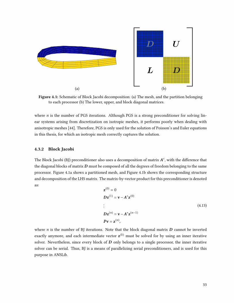
U

L D

D

(a) (b)

Figure 4.1: Schematic of Block Jacobi decomposition: (a) The mesh, and the partition belongingto each processor (b) The lower, upper, and block diagonal matrices.

where n is the number of PGS iterations. Although PGS is a strong preconditioner for solving lin-ear systems arising from discretization on isotropic meshes, it performs poorly when dealing withanisotropic meshes [44]. Therefore, PGS is only used for the solution of Poisson’s and Euler equationsin this thesis, for which an isotropic mesh correctly captures the solution.

4.3.2 Block Jacobi

The Block Jacobi (BJ) preconditioner also uses a decomposition of matrix A∗, with the dierence thatthe diagonal blocks of matrixD must be composed of all the degrees of freedom belonging to the sameprocessor. Figure 4.1a shows a partitioned mesh, and Figure 4.1b shows the corresponding structureand decomposition of the LHS matrix. The matrix-by-vector product for this preconditioner is denotedas:

z(0) = 0

Dz(1) = v−A∗z(0)

...

Dz(n) = v−A∗z(n−1)

P v = z(n),

(4.13)

where n is the number of BJ iterations. Note that the block diagonal matrix D cannot be invertedexactly anymore, and each intermediate vector z(k) must be solved for by using an inner iterativesolver. Nevertheless, since every block of D only belongs to a single processor, the inner iterativesolver can be serial. Thus, BJ is a means of parallelizing serial preconditioners, and is used for thispurpose in ANSLib.

33

4.3.3 ILU

The incomplete lower-upper factorization with ll level p (ILUp) produces an approximation of the LUfactorization of A∗, such that the approximate matrices have a much smaller nonzero structure thanthe exact LU factorization. The factored lower and upper triangular matrices L and U are computed byperforming Gaussian elimination on A∗, but ignoring certain matrix entries. Then, the preconditionermatrix is set to P = (LU )−1. A larger ll level results in L and U matrices with bigger nonzerostructure, but is likely to construct a more eective preconditioner [63]. Nevertheless, the ILU methodis inherently a serial algorithm, so it is implemented in conjunction with the BJ method for parallelsimulations.

Since the ILU preconditioner is based on matrix factoring, its performance is dramatically aectedby the ordering of DOFs in the matrix A∗. Quotient minimum degree (QMD) and reverse Cuthill-McKee (RCM) are among the reordering algorithms that are oered in PETSc [10], and are used inANSLib. The former reduces the ll of the factored matrices, while the latter reduces the ll of matrixA∗ itself.

In the course of development of ANSLib, Nejat and Ollivier-Gooch [49] used an ILU preconditionerfactored from the LHS matrix of the 0-exact scheme to solve the Euler equations. They showed thegood performance of their preconditioning method for 1- and 2-exact nite volume schemes, but con-cluded that the 3-exact scheme requires a more eective preconditioner. Later, Michalak and Ollivier-Gooch [47] demonstrated that incomplete factorization of the higher-order LHS matrix results in fasterconvergence compared to factoring the 0-exact LHS matrix for inviscid problems. They further con-jectured that factoring the LHS matrix to the full order using a ll level of 3 has a feasible memoryconsumption, and can be a practical preconditioner for three-dimensional ow problems. Hereinafter,the ILU preconditioner of ll level p factored from the 0-exact and full-order LHS matrices will bedenoted as LO-ILUp and HO-ILUp, respectively.

Viscous ow problems are more challenging than their inviscid counterparts. Jalali and Ollivier-Gooch[32] observed that a ll level of three or larger is required for HO-ILU preconditioning of viscous turbu-lent ow problems. The HO-ILU3 method is a practical preconditioner for two-dimensional problems,but its memory cost soars drastically in three-dimensions, hindering its implementation for such prob-lems. To mitigate this issue, a new ILU based algorithm will be introduced in the next section that notonly has a less memory consumption than HO-ILU3, but also does not suer from poor performanceof LO-ILU when used with the 3-exact reconstruction scheme.

4.4 Improved Preconditioning Algorithms

In this section, an eective preconditioning algorithm is proposed based on inner GMRES iterations.Furthermore, the lines of strong unknown coupling are presented for reordering of the LHS matrix.As will be shown in Section 4.5, this reordering method can improve the speed of the solver consider-

34

ably.

4.4.1 Inner GMRES Iterations

Some researchers have observed that the lower-order LHS matrix can construct a more eective pre-conditioner compared to its higher-order counterpart because the structure of the lower-order LHSmatrix only includes the immediate neighbors of every control volume [41, 56, 78]. Nevertheless, aswill be shown in Section 4.5, the LO-ILU method can behave poorly for high-order reconstructionschemes applied to viscous ow problems. Our conjecture is that using the exact inverse of the lower-order LHS matrix as the preconditioner: P = (A∗)−1, rather than the product of the ILU matrices:P = (LU )−1, can mitigate the mentioned issue. In this case, the matrix-by-vector product z = P v canbe found by solving the system:

A∗z = v. (4.14)

Nevertheless, the linear system of Equation (4.14) can be as large as the original linear system Ax = b,and its solution cannot be carried out exactly. Instead of seeking the exact solution, the proposal isto use further inner ILU preconditioned GMRES iterations to nd an approximate solution for Equa-tion (4.14). The resulting preconditioner will be referred to as GMRES-LO-ILU in this thesis, and itsperformance will be examined in Section 4.5.

When an inner GMRES solver is used as the preconditioner, P will not be a linear operator anymore,and its eect changes from iteration to iteration. Therefore, the equation x(m) = P Vmαm cannot beused any longer. The solution to this issue is using a Flexible GMRES (FGMRES) outer solver [62].The resulting combination, i.e., a GMRES-LO-ILU preconditioned FGMRES solver, is shown in Al-gorithm 2. Unlike normal GMRES, the z vectors are found by applying the inner GMRES solver tothe v vectors, and are explicitly kept track of as the columns of the Z matrix. Moreover, the nalapproximate solution is written as x(m) = Zmαm while the ILU factored matrices are still supplied tothe algorithm for preconditioning the inner GMRES solver. Also, tolerance values and limits for themaximum number of iterations have to be specied for both the inner and outer solvers which areidentied by the subscripts (.)i and (.)o, respectively.

4.4.2 Lines of Strong Coupling Between Unknowns

Forming non-overlapping lines that contain control volumes with strongly coupled degrees of free-dom is benecial in constructing eective preconditioners. Mavriplis [43] introduced the concept oflines in anisotropic unstructured meshes to enhance the performance of multigrid solvers via implicitsmoothing. His approximate algorithm for nding such lines was purely geometric-based, and onlyconsidered control volume aspect ratios. Thus, his method only captured coupling through diusion.Okusanya et al. [52] later developed an algorithm that considered both the advection and diusion phe-nomena. Fidkowski et al. [21] proved that such an algorithm results in a set of unique lines, and used

35

Algorithm 2 GMRES-LO-ILU preconditioned FGMRES with no restart and a zero initial guess.function FGMRES(A,A∗, L, U ,b,no,rtolo,ni ,rtoli )

β = ‖b‖2v1 = b/βV1 = [v1], H0 = [], Z0 = [],m = 0repeat

m =m+1zm =GMRES(A∗, (LU )−1,vm,ni ,rtoli )w = Azmhm,vm+1 = Arnoldi(Vm,w)Vm+1 = [Vm,vm+1], Hm = [Hm−1,hm], Zm = [Zm−1,zm]αm,γm =DenseSolve(β,Hm)

until m > n or γm/β < rtolReturn x(m) = Zmαm

the lines for nonlinear p-multigrid solution of Euler equations. Diosady and Darmofal [20] showedthat reordering the unknowns, such that members of a line have consecutive numbers, is an eectivereordering strategy for the ILU preconditioner. In this thesis, the line reordering algorithm of [20] isimplemented to improve the speed of the linear solver.

In the rst step of the line creation algorithm, a weight is assigned to every face inside the mesh.This weight is derived from the Jacobian of the 0-exact discretization of the advection-diusion equa-tion,

∇ · (vu −µL∇u) = 0, (4.15)

where u is the unknown variable, v is the velocity taken from the initial conditions, and µL is an inputparameter that controls the sensitivity of the lines to mesh anisotropy. The weight of a face f is thendened as:

W (f ) = max(∂Rσ∂uτ

,∂Rτ∂uσ

), (4.16)

where W is the weight of the face, σ and τ are the adjacent control volumes of the face, and R theresidual vector. If a face is located on the boundary, Equation (4.16) will not directly be applicable toit. Thus, a mirrored ghost control volume is placed adjacent to every boundary face. After ndingthe face weights, calling Algorithm 3 will construct the lines, where F(τ) is the set of faces of controlvolume τ , and σ = C(τ,f ) is the control volume which has the face f in common with control volumeτ . This algorithm ensures that two adjacent control volumes are connected to each other if and onlyif they have their rst or second highly weighted face lying between them [21].

To illustrate the performance of the algorithm, an anisotropic mesh for the geometry of a NACA 0012airfoil is considered, as shown in Figure 4.2. The velocity has been taken from the 2-exact solution ofthe ow resulting from a Mach number of 0.15, a Reynolds number of 6×106, and an angle of attackof 10. The parameter µL is set to the heuristic value of 10−5. As desired, the lines follow the direction

36

Algorithm 3 Line creationfunction CreateLines . Calling this function creates all lines.

Unmark all control volumes.while there a exists an unmarked control volume τ do

MakePath(τ) . Forward path creationMakePath(τ) . Backward path creation

function MakePath(τ) . Helper function.repeat

For control volume τ , pick the face f ∈ F(τ) with the highest weight, such that controlvolume σ = C(τ,f ) is not part of the current line.if f is a boundary face then

Terminateelse if σ is marked then

Terminateelse if f is not the rst or second ranked face of σ in weight then

TerminateMark σ .Add σ to the current line.τ← σ

until Termination

of mesh anisotropy near wall boundaries, while their pattern changes, and follows the ow directionin other parts of the geometry.

4.5 Numerical Comparisons

In this section, the performance of the proposed preconditioning algorithm is studied by consider-ing the turbulent ow around a NACA 0012 airfoil, with α = 10, Ma = 0.15, and Re = 6 × 106.Three nested meshes with approximately 25K, 100K, and 400K control volumes (NCV = 25K,100K,and 400K) are considered, where the coarsest mesh and its corresponding lines of strong unknowncoupling are shown in Figure 4.2. The fareld boundaries are located almost 500 chords away fromthe airfoil, and the chord length has a nondimensional value of one. This problem is taken from theNASA Turbulence Modeling Resource (TMR) website [60], and has been previously studied by Jalaliand Ollivier-Gooch [32], where they used a HO-ILU3 preconditioner with QMD reordering. Onlythe highest-order discretization scheme of ANSLib (3-exact) is considered here, since it results in thestiest linear systems that are most dicult to solve. Also, the initial conditions are taken from thesteady-state solution of the lower-order 2-exact scheme.

The ILU based preconditioning methods tested are shown in Table 4.1. In all cases, the outer GMRESsolver stops when the linear residual of Equation (4.3) is reduced by a factor of 10−3, or a maximumnumber of 500 iterations is performed. The maximum Krylov subspace size is 100 for the outer GMRES

37

Block Color

Figure 4.2: Mesh and lines of strong unknown coupling for the geometry of a NACA 0012 airfoil

38

Table 4.1: Preconditioning methods considered

Case Preconditioning Reorderingrtoli ,niname method algorithm

A HO-ILU3 QMD —B LO-ILU0 RCM —C LO-ILU0 lines —D GMRES-LO-ILU0 RCM 10−3,10E GMRES-LO-ILU0 lines 10−3,10E∗ GMRES-LO-ILU0 lines 10−3,60

0.0 0.2 0.4 0.6 0.8 1.0Wall time (s)

0.0

0.2

0.4

0.6

0.8

1.0

|R(U

h)|2

0 200 400 600 80010−6

10−4

10−2

100

102

104

NCV=25K

0 1000 2000 3000 4000 5000

NCV=100KCase ACase BCase CCase DCase E

Figure 4.3: Comparison of residual histories for the NACA 0012 problem obtained using dierentpreconditioning algorithms

solver, and the initial CFL number is set to 10−2. Furthermore, the simulation ends when the normof the residual vector ‖R(Uh)‖2 is reduced by a factor of 10−8. The command-line options supplied tothe ANSLib executable for each case are listed in Appendix A. Cases A-E are compared to each otheron the 25K and 100K meshes, while case E∗ is used to solve the problem on the nest mesh. Note thatother combinations of preconditioner and reordering schemes that are not considered in Table 4.1,did not result in convergence even for the coarse mesh. Moreover, an extensive search for ndingthe optimum number of inner iterations ni has not been carried out, and the large number of inneriterations for case E∗ is chosen as a safe measure to ensure convergence on the nest mesh.

The residual history of the solver for each preconditioning algorithm is shown in Figure 4.3, wherethe wall time is obtained from a single core of an Intel i7-4790 (3.60 GHz) CPU. Our proposed pre-conditioning algorithm (case E) outperforms all the other methods on both mesh sizes, and takes onlyhalf the time of the HO-ILU3 algorithm (case A) to nd the steady-state solution. Furthermore, theline reordering algorithm shows its prominence on the 100K control volume mesh, where the RCMreordering algorithm fails. The eectiveness of the new preconditioning algorithm is further demon-strated by solving the problem on a 400K control volume mesh. The residual history for this case isshown in Figure 4.4.

39

0 5×104 1×105

Wall time (s)

10-6

10-4

10-2

100

102

‖R(U

h)‖

2

case E ∗

Figure 4.4: Residual history for the NACA 0012 problem on the nest mesh of 400K controlvolumes

Table 4.2 shows the number of PTC iterations (N-PTC), the number of outer GMRES iterations (N-GMRES), total memory consumption, CPU time spent on the linear solver (LST), and total computa-tional time (TST). The proposed preconditioning scheme (case E) speeds up the linear solve process bya factor of three, and results in a twofold reduction in memory consumption, compared to the HO-ILU3method. The shortcomings of the LO-ILU methods (cases B and C) are evident because of their largenumber of PTC iterations and failure in convergence, on the coarse and medium meshes, respectively.Also, the memory consumption scales linearly with respect to the problem size for the proposed pre-conditioning scheme, whereas the linear solve time seems to be increasing at a much more rapid rate.Although the proposed preconditioning scheme has a huge linear solve time for NCV = 400K, it stilloutperforms the HO-ILU3 method, which cannot handle this mesh size at all.

The viscous drag (CDv), the pressure drag (CDp), and the lift (CL) coecients computed from thenumerical solution along with their reference values are listed in Table 4.3. The reference values aretaken from the NASA TMR website, and are obtained by the FUN3D [2] solver running on a veryne mesh (approximately 2M quadrilaterals). As expected, the change in the coecients between thene and medium meshes is much smaller than that of the medium and coarse meshes. Furthermore,the gap between the coecients and their reference values gets smaller with mesh renement, withthe exception of CL. Solution singularities, dierent boundary condition implementations betweenANSLib and FUN3D, or inexact evaluation of the distance from wall function may partly be accountablefor the non-ideal behavior of the lift coecient. Nevertheless, the purpose of this section was thesolution of the discretized system of equations, which according to Figure 4.4 has been performedcorrectly.

40

Table 4.2: Performance comparison for dierent preconditioning schemes. Cases with entriesmarked by “−” did not converge to the steady state solution.

Preconditioner N-PTC N-GMRES Memory(GB) LST(s) TST(s)NCV = 25K

A 37 956 1.4 416 635B 44 10,893 0.7 264 572C 51 13,692 0.7 328 705D 34 1,856 0.7 134 379E 34 1,787 0.7 118 361

NCV = 100KA 39 4,640 5.9 3,122 4,068B − − 2.8 − −C − − 2.8 − −D − − 3.2 − −E 36 4,396 3.2 1,308 2,348

NCV = 400KE∗ 38 6,869 13.1 87,312 91,502

Table 4.3: Computed drag and lift coecients for the NACA 0012 airfoil

NCV CDp CDv CL25K 0.00545 0.00583 1.0951100K 0.00615 0.00623 1.0905400K 0.00609 0.00619 1.0922

NASA TMR 0.00607 0.00621 1.0910

41

Chapter 5

Three-Dimensional Results

This chapter presents the k-exact nite volume solution of four three-dimensional problems. Theproblems are studied in order of diculty, and the solutions are veried to assess the accuracy andperformance of the solver. First, Poisson’s equation is solved in a cubic domain, where the source termis obtained from a manufactured solution [64]. Then, the Euler equations are solved to simulate thesubsonic inviscid ow around a unit sphere. Subsequently, the solution of Navier-Stokes + negativeS-A equations are presented to simulate the subsonic viscous turbulent ow over a at plate and theextruded NACA 0012 airfoil. All the command-line options provided to the solver for running eachcase are provided in Appendix A.

All the ow simulations were performed using the Grex cluster from the WestGrid computing facilities[3]. Each node of the cluster consists of two 6-core Intel Xeon X5650 2.66GHz processors, and has aminimum of 48GB memory. All compute nodes are connected by a non-blocking Inniband 4X QDRnetwork. The wall time and memory cost of all the ow problems are reported using 8 processors.In addition, a strong parallel scaling test is conducted for the at plate and the sphere test cases, i.e.,the same problem is solved by using dierent numbers of processors ranging from 1 to 10 while theresulting speedup is recorded.

5.1 Poisson’s Equation in a Cubic Domain

For this test case, Poisson’s equation is considered inside the domain Ω = [0,1]3. The manufacturedexact solution

u = sinh(sin(x1))sinh(sin(x2))sinh(sin(x3)) (5.1)

is used to nd the source term, while homogeneous Dirichlet conditions are imposed over all theboundaries. Slice plots of the exact solution are shown in Figure 5.1. The solution has a maximumvalue of (sinh(1))3 at the point (12 ,

12 ,

12 ), and decays to zero on the boundaries.

A study of the solution accuracy is performed on four families of unstructured grids. The rst grid

42

Figure 5.1: Exact solution of Poisson’s problem

family is only composed of hexahedra while the other families are composed of only prisms, mixtureof pyramids and tetrahedra, and only tetrahedra, respectively. The hexahedral grids are constructed byperturbing the vertices of a uniformN ×N ×N structured mesh. Other grid families are subsequentlycreated by decomposing each hexahedron into the desired element types. Figure 5.2 shows all the gridsfor N = 5.

The problem is solved on grid sizes: N = 10,20,40, and reconstruction orders: k = 1,2,3. Figure 5.3shows the L2 norm of the discretization error ‖eh‖2 as a function of the mesh length scale h = 1

N andthe number of degrees of freedom. Optimal accuracy order of k + 1 is attained for the k = 1 and 3

reconstruction schemes as expected, whereas the k = 2 scheme only achieves a second-order accuratesolution. Nevertheless, the non-optimal behavior of k = 2 is expected for Poisson’s problem, and waspreviously addressed and theoretically explained by Ollivier-Gooch and Van Altena [54].

5.2 Inviscid Flow Around a Sphere

The second test problem is the inviscid ow around a sphere with unit radius, and centered at the point(0,0,0). The Mach number is equal to Ma = 0.38, and the free-stream ow is in the x1 direction. Thisproblem is chosen as a three-dimensional extension of the inviscid ow around a circle, the higher-order solution of which was studied by Bassi and Rebay [14]. Three prismatic grids (64K, 322K, and 1Mcontrol volumes) are used, where the fareld is located at a distance of 100 dimensionless units fromthe sphere surface. A symmetric cut of the coarsest mesh near the sphere surface is shown in Figure 5.4.The faces and control volumes adjacent to the wall boundaries are curved using only second-orderLagrange polynomials, as quadratic functions are sucient to represent a spherical surface. To ensurethat numerical quadrature does not introduce additional error in the solution, a quadrature schemeaccurate up to order k +2 is employed.

43

(a) (b)

(c) (d)

Figure 5.2: Dierent meshes for the solution of Poisson’s problem: (a) hexahedra, (b) prisms, (c)mixture of pyramids and tetrahedra, (d) tetrahedra.

44

1 2 3 4h0/h

10−6

10−5

10−4

10−3

10−2

10−1

|e h| 2

k=1

1 2 3 4h0/h

k=2

1 2 3 4h0/h

k=3

Hex Prism Pyramid+Tet Tet O(h k+1)

(a)

103

104

105

106

NDOF

10−6

10−5

10−4

10−3

10−2

10−1

|e h| 2

k=1

103

104

105

106

NDOF

k=2

103

104

105

106

NDOF

k=3

(b)

Figure 5.3: Discretization error versus mesh size for Poisson’s problem: (a) Error versus meshlength scale, (b) Error versus number of degrees of freedom.

Figure 5.4: Symmetric cut of the coarsest mesh near the sphere surface

45

1 2 3 4 5 6h0/h

10-7

10-6

10-5

10-4

10-3

‖Sh−S∞‖ 2

ave. slope=2.2

ave. slope=2.4

ave. slope=4.8

k=1

k=2

k=3

Figure 5.5: Relative entropy norm versus mesh size for the sphere problem

In all cases, the initial solution is the uniform free-stream condition everywhere, and the initial CFLnumber is set to 10. The GMRES linear solver stops when the linear residual of Equation (4.3) is 10−3

times its initial value, or a maximum of 500 iterations is performed. Furthermore, the GMRES solverhas a maximum Krylov subspace size of 100, and is preconditioned using the BJ preconditioner withno = 4 iterations. The inner solver for the BJ preconditioner is PGS with ni = 4 iterations. Althoughthe LHS matrix of the linear system is calculated to full-order, its preconditioner is constructed fromthe LHS matrix of the 0-exact reconstruction scheme.

As the ow does not contain any discontinuity, the entropy must be constant throughout the domain.Therefore, the L2 norm of the entropy relative to the free-stream conditions, ‖S − S∞‖2, has an exactvalue of zero, and is used to study the solution accuracy. The convergence of ‖S − S∞‖2 with meshrenement is shown in Figure 5.5, where the mesh length scale is dened as h = (NCV)−1/3. The k = 1

and 3 reconstruction schemes converge even faster than their expected ratios of 2 and 4, respectively.The convergence ratio for the k = 2 reconstruction scheme, however, is half an order smaller than itsnominal value. The slight deviation of the convergence orders from their theoretical values can partlybe attributed to the fact that the meshes employed are not nested.

The eect of the reconstruction order k on solution accuracy is also evident from the qualitative Machcontours on the x3 = 0 symmetry plane, shown in Figure 5.6. Not surprisingly, only the k = 3 re-construction scheme has been able to capture the symmetry of the ow on the nest mesh. Further-more, the articial wake behind the sphere seems smaller for the k = 2 solution compared to that ofk = 1.

The norm of the residual vector per PTC iteration is shown in Figure 5.7. Convergence is independentof the reconstruction order k, but the number of iterations increases as the mesh is rened. It isnoteworthy to mention that the increase in the initial norm corresponding to mesh renement is dueto the denition of the residual vector R(Uh) in Equations (2.3) and (2.4). Each entry of the residualvector is divided by the size of its corresponding control volume. Therefore, when the mesh is rened,

46

NCV = 64K NCV = 1Mk=1

k=2

k=3

Figure 5.6: Computed Mach contours on the x3 = 0 symmetry plane for the sphere problem

47

0.0 0.2 0.4 0.6 0.8 1.0PTC iteration

0.0

0.2

0.4

0.6

0.8

1.0

0 10 2010-12

10-10

10-8

10-6

10-4

10-2

100

102

‖R(U

h)‖

2

k=1

0 10 20

k=2

0 10 20

k=3 NCV = 64K

NCV = 322K

NCV = 1M

Figure 5.7: Norm of the residual vector per PTC iteration for the sphere problem

Table 5.1: Number of iterations and the resource consumption of the ow solver for the sphereproblem

k N-PTC N-GMRES Memory(GB) LST(s) TST(s)NCV = 64K

1 15 182 2.94 24 1072 15 181 3.91 20 1123 15 255 6.00 31 320

NCV = 322K1 16 207 13.24 134 5792 16 212 14.05 132 6203 16 300 28.39 271 1,879

NCV = 1M1 17 275 39.48 486 1,9692 17 277 45.52 536 2,1503 17 385 85.78 793 5,904

the control volume sizes become smaller, and the residual vector entries will increase.

The number of iterations and the resource consumption of the ow solver are listed in Table 5.1. Thetime spent on linear solves makes up less than twenty percent of the computational time, suggestingthat the Jacobian evaluation is the major computational bottleneck for this problem. Either increas-ing the reconstruction order, or the number of control volumes results in stier linear systems, whichrequire more GMRES iterations to be solved. Nevertheless, both the solution time and memory con-sumption increase linearly with the number of control volumes for all k. Also, the advantage of usinga high-order reconstruction scheme can be clearly seen: According to Figure 5.5, the k = 1 schemeneeds at least one level of uniform mesh renement on the nest grid to achieve an entropy norm of10−7. While such a mesh renement would increase the resource consumption by a minimum factorof eight, the k = 3 scheme achieves the same level of accuracy by consuming only two times the sameresources.

48

1 2 3 4 5 6 7 8 9 10# of processors

1

2

3

4

5

6

7

8

9

10

Speed-up

Ideal

Total

Jac. int.

Lin. solve

Figure 5.8: The parallel speedup of the solver for the sphere problem: NCV = 322K and k = 3.

To test the parallel scalability of the ow solver, the sphere problem was solved on dierent numbers ofprocessors ranging from 1 to 10 withNCV = 322K and k = 3. The parallel speedup of the total solutionprocess, the Jacobian evaluation algorithm, and the linear solver scheme were computed separately,and are shown in Figure 5.8. Not surprisingly, the linear solver algorithm is less scalable than that ofthe Jacobian integrator mainly because the performance of the BJ preconditioner decreases with anincrease in the number of processors. The sudden dip of the parallel speedup for 9 processors may bedue to a less favorable mesh partitioning, or communication problems on the cluster. Regardless, theoverall solution algorithm scales very well in parallel, as the linear solver only constitutes a small partof the overall process.

5.3 Turbulent Flow Over a Flat Plate

For this test case, we consider a three-dimensional extension of the at plate verication case fromthe NASA TMR website. The computational domain is Ω = [−0.33,2]× [0,1]× [0,1], and the nondi-mensional parameters have the values: Re = 5 × 106, Ma = 0.2, α = 0, and ψ = 0. The at plateis located on the (0 ≤ x1 ≤ 2)∧ (x2 = 0) boundary, where adiabatic solid wall conditions are imposed.Symmetry boundary conditions are imposed on the (x3 = 0), (x3 = 1), and (−0.33 ≤ x1 ≤ 0)∧ (x2 = 0)

boundaries, while other boundaries are considered as fareld. As symmetry boundary conditions areimposed on all the boundaries normal to the x3-axis, the exact solution of this problem must be con-stant in the x3 direction. Therefore, the solutions obtained in this section can be compared to thetwo-dimensional results from the NASA TMR website, which are obtained by the CFL3D solver [1] ona 544× 384 grid.

The two-dimensional meshes provided by the NASA TMR website are extruded in the x3 directionto construct a series of nested three-dimensional grids with dimensions: 60 × 34 × 7, 120 × 68 × 14,and 240 × 136 × 28. The coarsest mesh is depicted in Figure 5.9. An anisotropic mesh is necessary

49

X

Y

Z

Figure 5.9: Coarsest mesh for the at plate problem.

to correctly capture the ow pattern in the boundary layer and at the plate leading edge. On eachmesh, the problem is solved for k = 1, then for k = 2, and nally for k = 3. The free-stream con-ditions are used as the initial conditions for k = 1, while the initial solution for each k ≥ 2 is takenfrom the converged solution of the (k − 1)-exact scheme. The GMRES-LO-ILU2 method is used as thepreconditioner, with 10 inner GMRES iterations, and the RCM reordering algorithm. Moreover, theILU factorization is performed only on the diagonal block of each processor. Other solver parametersare the same as Section 5.2.

To schematically demonstrate the correctness of the solution, the distribution of the turbulence work-ing variable obtained from k = 3 on the nest mesh is plotted on the x3 = 0.5 plane, and shown in Fig-ure 5.10a. The results for a 544×384 grid provided by the NASA TMR are also shown in Figure 5.10b.There is a close agreement between the reference solution of NASA TMR and the solution of this thesis,although a few undershoots of small magnitude are present in the latter. The next quantity of interestis the distribution of the nondimensional eddy viscosity µT

µ on the line (x1 = 0.97)∧ (x3 = 0.5), whichis depicted in Figure 5.11. Note how the solution discontinuity at control volume boundaries is quiteevident for k = 1, while higher-order reconstruction schemes result in much smoother solutions. Thereference solution from the NASA TMR website is also shown in Figure 5.11. An acceptable agree-ment is observable between our computed results and the reference values. Also, it is evident that ahigher-order reconstruction scheme leads to a more accurate estimate of the eddy viscosity.

To further verify the numerical solution, the convergence of the drag coecient CD and the skinfriction coecientCf at the point x = (0.97,0,0.5) are studied with mesh renement. Table 5.2 showsthe computed values on dierent meshes. The computed values converge faster for a higher-orderreconstruction scheme, such that only k = 3 oers an accurate solution on the medium mesh. Thereference values from the NASA TMR library are also shown in the same table. As desired, there is agood agreement between the computed values using the method of this thesis and the reference values

50

(a) 3-exact: min : 7× 10−3, max : 379 (b) NASA TMR: min : 0, max : 378

Figure 5.10: Distribution of the turbulence working variable on the plane x3 = 0.5 for the atplate problem

0.0 0.2 0.4 0.6 0.8 1.00.0

0.2

0.4

0.6

0.8

1.0

x2

0.00

0.01

0.02

0.03

60×34×7NASA TMRk=1

k=2

k=3

0.00

0.01

0.02

0.03

120×68×14

0 50 100 150 200 250µT/µ

0.00

0.01

0.02

0.03

240×136×28

Figure 5.11: Distribution of the nondimensional eddy viscosity on the line (x1 = 0.97)∧ (x3 =0.5) for the at plate problem

51

Table 5.2: Computed value and convergence order of the drag coecient and the skin frictioncoecient at the point x = (0.97,0,0.5) for the at plate problem

CD CfNASA TMR 0.00286 0.00271

Meshk

1 2 3 1 2 3

60× 34× 7 0.00396 0.00233 0.00233 0.00350 0.00228 0.00222120× 68× 14 0.00301 0.00281 0.00285 0.00283 0.00268 0.00271240× 136× 28 0.00287 0.00286 0.00286 0.00274 0.00273 0.00273

Convergence order 2.8 3.3 5.4 3 3 5.1

0 10 20 30 40 50 60 70 80 90PTC iteration

10-9

10-7

10-5

10-3

10-1

101

103

105

‖R(U

h)‖

2

k=1 k=2 k=360×34×7

120×68×14

240×136×28

Figure 5.12: Norm of the residual vector per PTC iteration for the at plate problem

of the NASA TMR website. The convergence orders ofCD andCf are computed using the procedure ofCelik et al. [16], and are also shown in Table 5.2. All the reconstruction schemes have attained optimalconvergence rates. Nevertheless, care must be taken when interpreting the estimated convergencerates because the procedure of Celik et al. is most reliable when the error has already achieved anasymptotic behavior on the coarsest mesh, which might not necessarily be the case here.

The norm of the residual vector per PTC iteration is shown in Figure 5.12. Similar to Section 5.2,convergence is not aected by the reconstruction order k, but is slightly degraded as the number ofdegrees of freedom increases. The number of iterations and the resource consumption of the owsolver are listed in Table 5.3. The majority of the total time is spent on linear solves, showing thatthe linear systems arising from viscous turbulent ows are much stier compared to their inviscidcounterparts. As desired, memory consumption increases linearly with mesh renement, whereas thelinear solve time does not scale as nicely as for the inviscid sphere problem. Most importantly, thebenet of higher-order methods can once again be observed: While the k = 3 solution on the mediummesh oers the same level of accuracy as the k = 1 solution on the ne mesh, the computational timeof the former is smaller than that of the latter by a factor of four.

52

Table 5.3: Number of iterations and the resource consumption of the ow solver for the at plateproblem

k N-PTC N-GMRES Memory(GB) LST(s) TST(s)60× 34× 7 mesh

1 26 844 0.42 31 552 26 1,009 1.35 42 1243 26 1,071 2.10 57 202

120× 68× 14 mesh1 28 1,436 5.24 510 7132 29 1,864 8.30 742 1,4893 29 2,041 14.63 825 2,124

240× 136× 28 mesh1 29 2,492 38.77 6,222 7,8842 27 3,305 60.70 12,353 18,1373 27 2,906 121.81 23,141 35,412

1 2 3 4 5 6 7 8 9 10# of processors

1

2

3

4

5

6

7

8

9

10

Speed-up

Ideal

Total

Jac. int.

Lin. solve

Figure 5.13: The parallel speedup of the solver for the at plate problem: 120 × 68 × 14 meshand k = 3.

A strong parallel scaling test is conducted for the k = 3 scheme on the 120 × 68 × 14 mesh. Theresulting speedup for dierent parts of the solver is shown in Figure 5.13, which is quite similar to theresults of the sphere problem, and suggests that the preconditioning algorithm is performing well forviscous ow problems. Nevertheless, the net scaling of the solver degrades marginally compared tothe sphere problem, as linear solves take up a bigger portion of the total solution time.

5.4 Turbulent Flow Over an Extruded Airfoil

For the last test case, we consider a three-dimensional extension of the ow around the NACA 0012 air-foil. The computational domain of Section 4.5 is extruded in the x3 direction with an extrusion length ofone nondimensional unit. Symmetry boundary conditions are imposed on the two boundaries normal

53

X

Y

Z

(a) Hexahedral mesh

X

Y

Z

(b) Mixed prismatic-hexahedral mesh

Figure 5.14: Meshes for the extruded NACA 0012 problem

to the x3-axis, while other boundaries retain their conditions from Section 4.5. The nondimensionalparameters are: Re = 6× 106, Ma = 0.15, α = 10, and ψ = 0. As the exact solution must be constantin the x3 direction, the solutions are compared to the reference values provided by NASA TMR, whichare obtained by the FUN3D [2] solver on a 7169× 2049 grid.

Two meshes are employed: a hexahedral mesh with NCV = 100K, and a mixed prismatic-hexahedralmesh withNCV = 176K. In both cases, quadrature points are obtained from the tensor product of one-dimensional quadrature formulas and the quadrature points of the curved two-dimensional meshes.A portion of the meshes is depicted in Figure 5.14. In both cases, there are 7 layers of extruded controlvolumes in the x3 direction. A value of MinNeigh(3) = 30 performed acceptably for the hexahedralmesh, whereas the same value resulted in an ill-conditioned version of Equation (2.7) for the mixedmesh. Therefore, MinNeigh(3) = 60 was used in the latter case as a safe measure to ensure a well-posed minimization problem for Equation (2.7). Other solver parameters, including the order rampingprocedure for solution initialization, are the same as Section 5.3.

The computed contours of turbulence working variable on the x3 = 0 plane are shown in Figure 5.15for the k = 3 solutions. The mixed-mesh resolves the wake region more accurately, while providinga smoother distribution of the turbulence working variable. The superior performance of the mixed

54

(a) Hexahedral mesh

(b) Mixed prismatic-hexahedral mesh

Figure 5.15: Distribution of the turbulence working variable for the extruded NACA 0012 prob-lem on the x3 = 0 plane

mesh can be explained by its bigger number of degrees of freedom, and the presence of extra owaligned faces that are missing in the hexahedral mesh.

The distribution of the surface pressure coecient on the intersection of the airfoil and the x3 = 0.5

plane is computed using the k = 1 and 3 solutions, and depicted in Figure 5.16. Generally, the computeddistributions are consistent with the reference values obtained by FUN3D. Closer views of the plots areshown for four distinct points to better compare the results. As expected, the k = 3 scheme predictsthe most accurate values, particularly on the mixed mesh. For example, the FUN3D results show thatthe pressure coecient on the lower surface becomes bigger than that of the upper surface, near thetrailing edge of the airfoil. This phenomenon is captured by the k = 3 solutions, but not observed bythose of k = 1.

The computed and the reference lift and drag coecients are shown in Table 5.4. It seems that thehexahedral mesh is too coarse, as none of the schemes can obtain accurate enough solutions. For themixed mesh, the k = 3 scheme gives satisfactory results with less than 10% error for all the coecients.The solution of the other schemes, however, is quite o, particularly for the pressure drag coecientCDp. Note that the reference results are obtained using a 7169 × 2049 mesh, which is more than athousand times ner than the meshes employed in this thesis.

The norm of the residual vector per PTC iteration is shown in Figure 5.17. Convergence is marginallyaected by either the mesh type or the reconstruction order k. The latter is a desirable result of usingthe steady-state solution of a k-exact scheme as the initial guess for the (k +1)-exact solution.

Finally, parameters related to the iterative convergence of the solver are listed in Table 5.5. The linear

55

0.0 0.2 0.4 0.6 0.8 1.0

x

−6

−5

−4

−3

−2

−1

0

1

2

Cp

(a)

(b)

(c)

(d)

FUN3Dk=3, hexk=3, mixedk=1, hexk=1, mixed

(a) (b)

(c) (d)

Figure 5.16: Distribution of surface pressure coecient on the intersection of the extrudedNACA 0012 airfoil and the x3 = 0.5 plane.

Table 5.4: Computed drag and lift coecients for the extruded NACA 0012 airfoil problem

k CDp CDv CLNASA TMR

− 0.00607 0.00621 1.0910Hex mesh

1 0.01703 0.00582 1.06192 0.01702 0.00497 1.05073 0.00301 0.00472 1.0417

Mixed mesh1 0.01129 0.00574 1.07352 0.00365 0.00565 1.07763 0.00550 0.00536 1.0869

56

0 20 40 60 80 100PTC iteration

10-7

10-5

10-3

10-1

101

103

105

‖R(U

h)‖

2

k=1 k=2 k=3

Hex

Mixed

Figure 5.17: Norm of the residual vector per PTC iteration for the extruded airfoil problem

Table 5.5: Resource consumption of the ow solver for the extruded NACA 0012 problem

k N-PTC N-GMRES Memory(GB) LST(s) TST(s)Hex mesh, NCV = 100K

1 33 1,154 4.77 317 7442 31 1,788 6.82 730 2,0973 31 2,415 12.23 1,057 3,215

Mixed mesh, NCV = 176K1 34 1,132 8.70 458 1,1642 32 1,769 10.87 800 2,4273 31 2,185 26.47 1,311 4,666

solve time makes up around 30% of the total computation time. The total computation time is stronglydependent on k, but does not dier considerably between the two meshes for the same reconstructionorder. Moreover, the memory consumption seems to be linearly increasing with both k andNCV.

57

Chapter 6

Conclusions

A higher-order solution framework was presented for steady-state three-dimensional compressibleows. The highlights of this solution framework include: a k-exact nite volume discretization, aPTC solution algorithm, a memory lean preconditioner based on inner GMRES iterations, and an ILUreordering algorithm based on lines of strong coupling between them.

Higher-order accuracy was achieved by constructing a piecewise continuous representation of thecontrol volume average values. This piecewise continuous representation, also referred to as the dis-crete solution, was dened as the superposition of a set of basis functions. Monomials of Cartesian,principal, or curvilinear coordinates were used as the basis functions while the coecient of eachmonomial in the superposition was found by solving a constrained minimization problem. In the -nite volume method, the convective uxes were evaluated by the Roe ux function. The viscous uxeswere obtained by adding a stabilizing damping term to the averaged gradients of the two adjacentstates. Specically, the ux functions were presented for the RANS equations fully coupled with thenegative S-A turbulence model.

The curvature of the domain boundaries must be correctly accounted for in high-order numericaldiscretization schemes, yet simply replacing the boundary faces of highly anisotropic meshes withhigher-order representations can result in invalid intersecting elements. Thus, a three-dimensionalnite element elasticity solver was developed to propagate the curvature of the boundary throughoutthe domain, and to prevent mesh tangling. The developed solver was tested by solving a model problemthat imitated the geometry of a three-dimensional airfoil. Also, the principal coordinates and thecurvilinear coordinates basis functions were presented to prevent the k-exact reconstruction schemefrom behaving poorly on curved anisotropic meshes.

The PTC method was revisited for the solution of the discretized nonlinear equations, where eachiteration required the solution of a linear system. The challenges involved in the solution of theselinear systems were addressed for three-dimensional problems, and a novel method was introducedto mitigate these issues. In this method, the FGMRES linear solver was preconditioned using inner

58

GMRES iterations, which were subsequently preconditioned by the ILU method. The L and U matri-ces were factored from the LHS matrix of the 0-exact discretization scheme, and the lines of strongunknown coupling were employed to reorder the unknowns. By considering the 2-D fully turbulentow around the NACA 0012 airfoil, it was shown that the proposed preconditioning algorithm is moreecient both in terms of solution time and memory consumption, compared to the other ILU basedpreconditioning methods considered.

The correct implementation of element quadrature and connectivity information in the solver wasveried by solving Poisson’s equation inside a cubic domain. Subsequently, inviscid and viscous tur-bulent test problems were considered, where the solution was veried against reference values eitherobtained analytically or provided by the NASA TMR website. In all cases, a satisfactory agreementwas observed between the solutions of this thesis and the reference values. Moreover, accuracy testswere performed with mesh renement, and optimal convergence order was attained for reconstruc-tion orders k = 1 and 3. The k = 2 scheme, however, was slightly inferior in performance comparedto its theoretical convergence order.

Timing results demonstrated the benet and practicality of using higher-order methods for obtaininga certain level of accuracy. A second-order discretization scheme required a ner grid and more com-putational time to attain the same level of accuracy compared to a higher-order discretization scheme.Furthermore, strong parallel scaling tests were performed, and excellent scaling was observed for theJacobian integration algorithm. The linear solver algorithm also demonstrated satisfactory parallelscaling results, although the performance in this area can still be improved. It was also observed thatthe required number of PTC iterations for convergence is independent of the reconstruction orderwhile only slightly aected by the grid size.

Much work remains to be done to extend the solution method of this thesis to solve industrially prac-tical problems:

1. A theoretical study can be conducted to investigate the inferior performance of the k = 2 dis-cretization scheme. The theoretical approach for unstructured mesh-based discretization meth-ods is usually through the functional analysis framework. A possible starting point can be thework of Barth and Larson [13] where they prove theoretical convergence orders for the k-exactnite volume method.

2. The boundary condition implementations of this work, though functional, might not be the bestchoice. An investigation of other possible boundary condition implementations has the potentialto improve convergence properties and solution quality [29].

3. The proposed preconditioning algorithm does not require the explicit form of the full-order LHSmatrix. Thus, a matrix-free method can be implemented, where the matrix-by-vector productof the full-order LHS matrix is evaluated by nite dierence Fréchet derivatives while only the0-exact LHS matrix is assembled. This strategy can reduce the memory cost considerably [55],while possibly increasing the computation time. Sacricing computation time for less memory

59

usage might be unavoidable for very large problems.

4. In this thesis, it was possible to directly use the 2-D curvilinear coordinate basis functions for 3-D problems, as the solutions of the test problems considered were constant in the x3 direction. Apractical problem, on the other hand, requires the denition of truly 3-D curvilinear coordinatebasis functions. It should be possible to generalize the method of Section 3.3 by providing adenition for the third wall coordinate. Alternatively, a big hexahedral meta-element can beconstructed by extruding a portion of the nearest wall surface to include all the members of atarget reconstruction stencil. The reference coordinates of the constructed meta-element canthen be used as the curvilinear coordinates.

5. The original 0-exact discretization scheme does not take the gradient dependent source termsinto account. Modifying this scheme to somehow capture the inuence of the gradient depen-dent source terms can greatly enhance the performance of the preconditioning algorithm [78].

6. Employing a line Gauss-Seidel preconditioner instead of the ILU method, in conjunction withthe proposed inner GMRES preconditioner has the potential to improve the parallel scalabilityof the linear solver [4].

7. As already mentioned, real world problems contain solution discontinuities, and require shockcapturing methods to be used in conjunction with the k-exact reconstruction scheme. Shockcapturing is even more important for higher-order methods, as they are more prone to develop-ing unstable and spurious solutions.

8. Haider et al. [26] recently introduced a multi-level reconstruction scheme that uses compactreconstruction stencils, and eliminates the need to directly work with large stencils. Their high-order nite volume method is therefore better suited for parallel simulations. Although theirwork is limited to the linear advection equation, its application in the context of turbulent com-pressible ows is worth investigating.

9. An hp-adaptive strategy can be much more ecient in achieving a prescribed level of accuracy,compared to uniform mesh renement, or using high reconstruction orders for all the controlvolumes [33, 38]. Desirably, hanging nodes resulting from adaptively rened meshes t natu-rally into the k-exact nite volume framework. Nevertheless, an eective error estimator mustbe designed that selects the candidate regions for renement. In the case of anisotropic meshrenement, the error estimator must also provide an estimate of the direction in which the errorchanges most abruptly.

60

Bibliography

[1] Computational Fluids Laboratory 3-D, 2011. URL hps://cfl3d.larc.nasa.gov/.

[2] Fully Unstructured Navier–Stokes in 3-D, 2011. URL hp://fun3d.larc.nasa.gov/.

[3] WestGrid computing resources, 2017. URL hps://www.westgrid.ca/.

[4] B. R. Ahrabi and D. J. Mavriplis. Scalable solution strategies for stabilized nite-element owsolvers on unstructured meshes. In Proceedings of the Fifty-Fifth AIAA Aerospace SciencesMeeting, page 517, 2017.

[5] B. R. Ahrabi, W. K. Anderson, and J. C. Newman III. An adjoint-based hp-adaptive stabilizednite-element method with shock capturing for turbulent ows. Computer Methods in AppliedMechanics and Engineering, 318:1030–1065, 2017.

[6] S. R. Allmaras, F. T. Johnson, and P. Spalart. Modications and clarications for theimplementation of the Spalart-Allmaras turbulence model. In Proceedings of the SeventhInternational Conference on CFD, 2012.

[7] P. R. Amestoy, I. S. Du, and J.-Y. L’Excellent. MUMPS multifrontal massively parallel solverversion 2.0. Technical report, CERFACS: Centre EuropÃľen de Recherche et de FormationAvancÃľe en Calcul Scientique, 1998. URL hp://mumps.enseeiht.fr/.

[8] J. Andren, H. Gao, M. Yano, D. Darmofal, C. Ollivier Gooch, and Z. Wang. A comparison ofhigher-order methods on a set of canonical aerodynamics applications. In Proceedings of theTwentieth AIAA Computational Fluid Dynamics Conference, page 3230, 2011.

[9] D. N. Arnold. An interior penalty nite element method with discontinuous elements. SIAMJournal on Numerical Analysis, 19(4):742–760, 1982.

[10] S. Balay, S. Abhyankar, M. F. Adams, J. Brown, P. Brune, K. Buschelman, L. Dalcin, V. Eijkhout,W. D. Gropp, D. Kaushik, M. G. Knepley, L. C. McInnes, K. Rupp, B. F. Smith, S. Zampini, andH. Zhang. PETSc users manual. Technical Report ANL-95/11 - Revision 3.6, Argonne NationalLaboratory, 2015. URL hp://www.mcs.anl.gov/petsc.

[11] G. E. Barter and D. L. Darmofal. Shock capturing with PDE-based articial viscosity forDGFEM: Part I. Formulation. Journal of Computational Physics, 229(5):1810–1827, 2010.

[12] T. J. Barth and P. O. Frederickson. Higher order solution of the Euler equations on unstructuredgrids using quadratic reconstruction. In Twenty-eighth AIAA Aerospace Sciences Meeting, Jan.1990. AIAA paper 90-0013.

61

[13] T. J. Barth and M. G. Larson. A posteriori error estimates for higher order Godunov nitevolume methods on unstructured meshes. Finite Volumes for Complex Applications III, London,2002.

[14] F. Bassi and S. Rebay. High-order accurate discontinuous nite element solution of the 2D Eulerequations. Journal of Computational Physics, 138(2):251–285, 1997.

[15] J. C. Butcher. Numerical Methods for Ordinary Dierential Equations. John Wiley & Sons, 2016.

[16] I. B. Celik, U. Ghia, and P. J. Roache. Procedure for estimation and reporting of uncertainty dueto discretization in CFD applications. Journal of Fluids Engineering-Transactions of the ASME,130(7), 2008.

[17] M. Ceze and K. J. Fidkowski. Constrained pseudo-transient continuation. International Journalfor Numerical Methods in Engineering, 102(11):1683–1703, 2015.

[18] S.-W. Cheng, T. K. Dey, and J. Shewchuk. Delaunay Mesh Generation. CRC Press, 2012.

[19] X. Deng, M. Mao, G. Tu, H. Zhang, and Y. Zhang. High-order and high accurate CFD methodsand their applications for complex grid problems. Communications in Computational Physics, 11(04):1081–1102, 2012.

[20] L. T. Diosady and D. L. Darmofal. Preconditioning methods for discontinuous Galerkin solutionsof the Navier–Stokes equations. Journal of Computational Physics, 228(11):3917–3935, 2009.

[21] K. J. Fidkowski, T. A. Oliver, J. Lu, and D. L. Darmofal. p-Multigrid solution of high-orderdiscontinuous Galerkin discretizations of the compressible Navier–Stokes equations. Journal ofComputational Physics, 207(1):92–113, 2005.

[22] J. E. Flaherty. Course notes on nite element analysis. URL hp://www.cs.rpi.edu/~flaherje/pdf.Accessed 05/12/17.

[23] S. K. Godunov. A nite dierence method for the numerical computation of discontinuoussolutions of the equations of uid dynamics. Matematicheskie Sborniki, 47:357–393, 1959.

[24] G. H. Golub and C. F. V. Loan. Matrix Computations. The Johns Hopkins University Press,Baltimore, 1983.

[25] F. Haider, J.-P. Croisille, and B. Courbet. Stability analysis of the cell centered nite-volumeMuscl method on unstructured grids. Numerische Mathematik, 113(4):555–600, 2009.

[26] F. Haider, P. Brenner, B. Courbet, and J.-P. Croisille. Ecient implementation of high orderreconstruction in nite volume methods. In Finite Volumes for Complex Applications VI Problems& Perspectives, pages 553–560. Springer, 2011.

[27] F. Haider, P. Brenner, B. Courbet, and J.-P. Croisille. Parallel implementation of k-exact nitevolume reconstruction on unstructured grids. In High-Order Nonlinear Numerical Schemes forEvolutionary PDEs, pages 59–75. Springer, 2014.

[28] A. Harten, P. D. Lax, and B. Van Leer. On upstream dierencing and Godunov-type schemes forhyperbolic conservation laws. In Upwind and High-Resolution Schemes, pages 53–79. Springer,1997.

62

[29] R. Hartmann and T. Leicht. Generation of unstructured curvilinear grids and high-orderdiscontinuous Galerkin discretization applied to a 3D high-lift conguration. InternationalJournal for Numerical Methods in Fluids, 2016.

[30] C. Hirsch. Numerical Computation of Internal and External Flows: Computational Methods forInviscid and Viscous Flows. Wiley, 1990.

[31] H. Huynh, Z. J. Wang, and P. E. Vincent. High-order methods for computational uid dynamics:a brief review of compact dierential formulations on unstructured grids. Computers and Fluids,98:209–220, 2014.

[32] A. Jalali and C. Ollivier-Gooch. Higher-order unstructured nite volume RANS solution ofturbulent compressible ows. Computers and Fluids, 143:32–47, 2017.

[33] A. Jalali and C. F. Ollivier Gooch. An hp-adaptive ustructured nite volume solver forcompressible aerodynamic ows. In Proceedings of the Fifty-Fifth AIAA Aerospace SciencesMeeting, page 0082, 2017.

[34] A. Jalali, M. Sharbatdar, and C. Ollivier-Gooch. Accuracy assessment of nite volumediscretization schemes on unstructured meshes. Computers and Fluids, 101:220–232, 2014.doi:10.1016/j.compfluid.2014.06.008.

[35] C. T. Kelley and D. E. Keyes. Convergence analysis of pseudo-transient continuation. SIAMJournal on Numerical Analysis, 35(2):508–523, 1998.

[36] B. S. Kirk, J. W. Peterson, R. H. Stogner, and G. F. Carey. libMesh: a C++ library for paralleladaptive mesh renement/coarsening simulations. Engineering with Computers, 22(3-4):237–254, 2006.

[37] W. M. Lai, D. H. Rubin, D. Rubin, and E. Krempl. Introduction to Continuum Mechanics.Butterworth-Heinemann, 2009.

[38] T. Leicht and R. Hartmann. Anisotropic mesh renement for discontinuous Galerkin methodsin two-dimensional aerodynamic ow simulations. International Journal for Numerical Methodsin Fluids, 56(11):2111–2138, 2008.

[39] S. K. Lele. Compact nite dierence schemes with spectral-like resolution. Journal ofComputational Physics, 103(1):16–42, 1992.

[40] W. Li. Ecient Implementation of High-Order Accurate Numerical Methods on Unstructured Grids.Springer, 2014.

[41] H. Luo, J. D. Baum, and R. Löhner. A fast, matrix-free implicit method for compressible ows onunstructured grids. In Sixteenth International Conference on Numerical Methods in FluidDynamics, pages 73–78. Springer, 1998.

[42] D. Mavriplis, D. Darmofal, D. Keyes, and M. Turner. Petaops opportunities for the NASAfundamental aeronautics program. In Proceedings of the Eighteenth AIAA Computational FluidDynamics Conference, page 4084, 2007.

[43] D. J. Mavriplis. Multigrid strategies for viscous ow solvers on anisotropic unstructuredmeshes. Journal of Computational Physics, 145(1):141–165, 1998.

63

[44] D. J. Mavriplis. Directional agglomeration multigrid techniques for high-Reynolds-numberviscous ows. AIAA Journal, 37(10):1222–1230, 1999.

[45] D. J. Mavriplis. Grid resolution study of a Drag Prediction Workshop conguration using theNSU3D unstructured mesh solver. In Proceedings of the Twenty-Third AIAA AppliedAerodynamics Conference, June 2005. AIAA paper 2005-4729.

[46] C. Michalak and C. Ollivier-Gooch. Accuracy preserving limiter for the high-order accuratesolution of the Euler equations. Journal of Computational Physics, 228(23):8693–8711, 2009.doi:10.1016/j.jcp.2009.08.021.

[47] C. Michalak and C. Ollivier-Gooch. Globalized matrix-explicit Newton-GMRES for thehigh-order accurate solution of the Euler equations. Computers and Fluids, 39:1156–1167, 2010.doi:10.1016/j.compfluid.2010.02.008.

[48] C. R. Nastase and D. J. Mavriplis. High-order discontinuous Galerkin methods using anhp-multigrid approach. Journal of Computational Physics, 213(1):330–357, 2006.

[49] A. Nejat and C. Ollivier-Gooch. A high-order accurate unstructured nite volumeNewton-Krylov algorithm for inviscid compressible ows. Journal of Computational Physics,227(4):2582–2609, 2008.

[50] H. Nishikawa. Beyond interface gradient: A general principle for constructing diusion scheme.In Proceedings of the Fortieth AIAA Fluid Dynamics Conference, 2010. AIAA paper 2010-5093.

[51] H. Nishikawa. Two ways to extend diusion schemes to Navier-Stokes schemes: Gradientformula or upwind ux. In Proceedings of the Twentieth AIAA Computational Fluid DynamicsConference, page 3044, 2011.

[52] T. Okusanya, D. Darmofal, and J. Peraire. Algebraic multigrid for stabilized nite elementdiscretizations of the Navier–Stokes equations. Computer Methods in Applied Mechanics andEngineering, 193(33):3667–3686, 2004.

[53] C. F. Ollivier-Gooch. Quasi-ENO schemes for unstructured meshes based on unlimiteddata-dependent least-squares reconstruction. Journal of Computational Physics, 133(1):6–17,1997.

[54] C. F. Ollivier-Gooch and M. Van Altena. A high-order accurate unstructured meshnite-volume scheme for the advection-diusion equation. Journal of Computational Physics,181(2):729–752, sep 2002. doi:10.1006/jcph.2002.7159.

[55] P.-O. Persson and J. Peraire. Newton-GMRES preconditioning for discontinuous Galerkindiscretizations of the Navier–Stokes equations. SIAM Journal on Scientic Computing, 30(6):2709–2733, 2008.

[56] A. Pueyo and D. W. Zingg. Ecient Newton-Krylov solver for aerodynamic computations.AIAA Journal, 36(11):1991–1997, 1998.

[57] P. Roe and J. Pike. Ecient construction and utilisation of approximate Riemann solutions. InProceedings of the Sixth International Symposium on Computing Methods in Applied Sciences andEngineering, VI, pages 499–518. North-Holland Publishing Co., 1985.

64

[58] P. L. Roe. Approximate Riemann solvers, parameter vectors, and dierence schemes. Journal ofComputational Physics, 43:357–372, 1981. doi:10.1016/0021-9991(81)90128-5. URLhp://www.sciencedirect.com/science/article/pii/0021999181901285.

[59] A. Rogerson and E. Meiburg. A numerical study of the convergence properties of ENO schemes.Journal of Scientic Computing, 5(2):151–167, 1990.

[60] C. Rumsey. Turbulence Modeling Resource, 2014. URL hp://turbmodels.larc.nasa.gov/.

[61] V. Rusanov. Calculation of Interaction of Non-steady Shock Waves with Obstacles. Technicaltranslation. National Research Council of Canada, 1962.

[62] Y. Saad. A exible inner-outer preconditioned GMRES algorithm. SIAM Journal on ScienticComputing, 14(2):461–469, 1993.

[63] Y. Saad. Iterative Methods for Sparse Linear Systems. SIAM, 2003.

[64] K. Salari and P. Knupp. Code verication by the method of manufactured solutions. Technicalreport, Sandia National Labs., Albuquerque, NM (US); Sandia National Labs., Livermore, CA(US), 2000.

[65] K. Shahbazi, D. J. Mavriplis, and N. K. Burgess. Multigrid algorithms for high-orderdiscontinuous Galerkin discretizations of the compressible Navier–Stokes equations. Journal ofComputational Physics, 228(21):7917–7940, 2009.

[66] C.-W. Shu. High order ENO and WENO schemes for computational uid dynamics. InHigh-order Methods for Computational Physics, pages 439–582. Springer, 1999.

[67] P. Solin, K. Segeth, and I. Dolezel. Higher-Order Finite Element Methods. CRC Press, 2003.

[68] P. Spalart and S. R. Allmaras. A one-equation turbulence model for aerodynamic ows. InThirtieth AIAA Aerospace Sciences Meeting, Jan. 1992. AIAA paper 92-0439.

[69] P. K. Sweby. High resolution schemes using ux limiters for hyperbolic conservation laws. SIAMJournal on Numerical Analysis, 21(5):995–1011, Oct. 1984. doi:hp://dx.doi.org/10.1137/0721062.

[70] E. Toro and A. Chakraborty. The development of a Riemann solver for the steady supersonicEuler equations. The Aeronautical Journal, 98(979):325–339, 1994.

[71] T. Toulorge, C. Geuzaine, J.-F. Remacle, and J. Lambrechts. Robust untangling of curvilinearmeshes. Journal of Computational Physics, 254:8–26, 2013.

[72] B. Van Leer. Towards the ultimate conservative dierence scheme. IV. A new approach tonumerical convection. Journal of Computational Physics, 23(3):276–299, 1977.

[73] B. Van Leer. Towards the ultimate conservative dierence scheme. V. A second-order sequel toGodunov’s method. Journal of Computational Physics, 135(2):229–248, 1997.

[74] J. Vassberg, M. DeHaan, and T. Sclafani. Grid generation requirements for accurate dragpredictions based on OVERFLOW calculations. In Proceedings of the Sixteenth AIAAComputational Fluid Dynamics Conference, page 4124, 2003.

[75] M. R. Visbal and D. V. Gaitonde. On the use of higher-order nite-dierence schemes oncurvilinear and deforming meshes. Journal of Computational Physics, 181(1):155–185, 2002.

65

[76] J. Von Neumann and R. D. Richtmyer. A method for the numerical calculation of hydrodynamicshocks. Journal of Applied Physics, 21(3):232–237, 1950.

[77] M. Wallra, R. Hartmann, T. Leicht, N. Kroll, C. Hirsch, F. Bassi, C. Johnston, and K. Hillewaert.Multigrid solver algorithms for DG methods and applications to aerodynamic ows. IDIHOM:Industrialization of High-Order Methods-A Top-Down Approach, 128:153–178, 2015.

[78] P. Wong and D. W. Zingg. Three-dimensional aerodynamic computations on unstructured gridsusing a Newton–Krylov approach. Computers and Fluids, 37(2):107–120, 2008.

[79] P. Woodward and P. Colella. The numerical simulation of two-dimensional uid ow withstrong shocks. Journal of Computational Physics, 54(1):115–173, 1984.

[80] S. H. Yoo, H. C. No, H. M. Kim, and E. H. Lee. CFD-assisted scaling methodology andthermal-hydraulic experiment for a single spent fuel assembly. Nuclear Engineering and Design,240(12):4008–4020, 2010.

66

Appendix A

ANSLib Command-Line Options

The command line interface provided by the ANSLib library consists of an executable le Solver, whichcan be executed through the Linux shell, with the input options provided in a separate text le:

$ ./Solver -opt < address of options file >

ANSLib achieves parallelism using the Message Passing Interface (MPI). Thus, parallel jobs can beexecuted via the MPI launcher :

$ mpiexec -np < # of processors > ./Solver -opt < address of options file >

In the remainder, the input options are presented for the test problems considered in this thesis. Notethat comments are distinguished by the character #, in the options le.

A.1 Two-Dimensional Turbulent Flow over a NACA 0012 Airfoilfrom Section 4.5

For this problem, several cases of preconditioners were considered. The following options are sharedbetween all the cases:

Common Options# --------------------------- MESH

-d 2 # Dimensions

-mesh_type c # Cell-centered mesh

-f < Location of .mesh file without extension >

-B < Location of .bdry file without extension >

-fec < Location of .fec file without extension >

# --------------------------- HISTORY AND SOLUTION FILE NAME

-sol < Location of initial solution input file >

-sol_out < Location of final solution output file >

-ita_history_name < Location of residual history output file >

67

# --------------------------- ACCURACY

-a < Order of accuracy of the scheme: a=k+1 >

# --------------------------- PHYSICS

-physics RoeTurbSA2D # 2-D RANS + negative S-A

-reynolds 6e6 # Reynolds number

-mach 0.15 # Mach number

-angle 10 # Angle of attack

# --------------------------- NON-LINEAR SOLVER OPTIONS

-exnut 1 # Ignore \tildenu entries in the line-search

-C 0.01 # Initial CFL number

-no_distance_weight # No distance weights in the k-exact

# reconstruction least squares problem

-pseudolts_fixed # No additional CFL ramping

-max_iter 80 # Maximum number of PTC iterations

-jacobian_type recanalytic # Evaluate the Jacobian exactly

-ita_target_residual 1e-5 # Target norm for the non-linear residual

To implement dierent preconditioning strategies, distinct sets of options have to be provided to theow solver in each case:

Extra Options for Case A# --------------------------- LINEAR SOLVER OPTIONS

# --------------------------- KSP

-ksp_max_it 500 # Maximum # of GMRES iterations

-ksp_rtol 1e-3 # rtol for the outer KSP

-ksp_type gmres # KSP solver type

# --------------------------- PC

-pc_type ilu # Preconditioner type: ILU

-pc_factor_levels 3 # ILU fill level: 3

-pc_factor_mat_ordering_type qmd # ILU reordering type: QMD

Extra Options for Case B# --------------------------- LINEAR SOLVER OPTIONS

# --------------------------- KSP

-ksp_max_it 500 # Maximum # of GMRES iterations

-ksp_rtol 1e-3 # rtol for the outer KSP

-ksp_type gmres # KSP solver type

# --------------------------- PC

-pre_order 1 # Order of scheme for A*

-pc_type ilu # Preconditioner type: ILU

-pc_factor_levels 0 # ILU fill level: 0

-pc_factor_mat_ordering_type rcm # ILU reordering type: RCM

Extra Options for Case C# --------------------------- LINEAR SOLVER OPTIONS

# --------------------------- KSP

68

-ksp_max_it 500 # Maximum # of GMRES iterations

-ksp_rtol 1e-3 # rtol for the outer KSP

-ksp_type gmres # KSP solver type

# --------------------------- PC

-mu 1e-5 # \mu_L for line construction

-pre_order 1 # Order of scheme for A*

-pc_type ilu # Preconditioner type: ILU

-pc_factor_levels 0 # ILU fill level: 0

-pc_factor_mat_ordering_type lines # ILU reordering type: LINES

Extra Options for Case D# --------------------------- LINEAR SOLVER OPTIONS

# --------------------------- KSP

-ksp_max_it 500 # Maximum # of GMRES iterations

-ksp_rtol 1e-3 # rtol for the outer KSP

-ksp_type fgmres # KSP solver type: FGMRES

# --------------------------- PC

-pre_order 1 # Order of scheme for A*

-pc_type ksp # Preconditioner type: inner-KSP

-ksp_ksp_type gmres # inner-KSP type: GMRES

-ksp_ksp_max_it 10 # inner-KSP n_i: 10

-ksp_pc_type ilu # inner-KSP preconditioner: ILU

-ksp_pc_factor_levels 0 # ILU fill level: 0

-ksp_pc_factor_mat_ordering_type rcm # ILU reordering: RCM

Extra Options for Case E# --------------------------- LINEAR SOLVER OPTIONS

# --------------------------- KSP

-ksp_max_it 500 # Maximum # of GMRES iterations

-ksp_rtol 1e-3 # rtol for the outer KSP

-ksp_type fgmres # KSP solver type: FGMRES

# --------------------------- PC

-mu 1e-5 # \mu_L

-pre_order 1 # Order of scheme for A*

-pc_type ksp # Preconditioner type: inner-KSP

-ksp_ksp_type gmres # inner-KSP type: GMRES

-ksp_ksp_max_it 10 # inner-KSP n_i: 10

-ksp_pc_type ilu # inner-KSP preconditioner: ILU

-ksp_pc_factor_levels 0 # ILU fill level: 0

-ksp_pc_factor_mat_ordering_type lines # ILU reordering: LINES

A.2 Poisson’s Equation from Section 5.1

69

# --------------------------- MESH

-d 3 # Dimensions

-mesh_type c # Cell-centered mesh

-f < Location of .vmesh file without extension >

# --------------------------- HISTORY AND SOLUTION FILE NAME

-sol_out < Location of final solution output file >

-ita_history_name < Location of residual history output file >

#---------------------------- PHYSICS

-physics Poisson # Solve Poisson’s equation

-poisson_problem_data sinhsin # Name of the manufactured solution

# --------------------------- ACCURACY

-a < Order of accuracy of the scheme: a=k+1 >

# --------------------------- NON-LINEAR SOLVER OPTIONS

-C 1e10 # Initial CFL number

-jacobian_type recanalytic # Evaluate the Jacobian exactly

-no_distance_weight # No distance weights in the k-exact

# reconstruction least squares problem

-max_iter 3 # Maximum number of PTC iterations

-ita_target_residual 1e-10 # Target norm for the residual vector R

# --------------------------- LINEAR SOLVER OPTIONS

-ksp_type gmres # KSP type: GMRES

-ksp_rtol 1e-12 # GMRES rtol

-pre_order 1 # Order of scheme for A*

-pc_type sor # Preconditioner type: PGS

-pc_sor_its 10 # Number of PGS iterations: 10

A.3 Inviscid Flow Over a Sphere from Section 5.2

# --------------------------- MESH

-d 3 # Dimensions

-mesh_type c # Cell-centered mesh

-f < Location of .vmesh file without extension >

# --------------------------- HISTORY AND SOLUTION FILE NAME

-sol_out < Location of final solution output file >

-ita_history_name < Location of residual history output file >

----------------------------- PHYSICS

-physics Euler3D # Solve 3-D Euler equations

-mach 0.38 # Mach number

-angle 0 # Angle of attack

# --------------------------- ACCURACY

-a < Order of accuracy of the scheme: a=k+1 >

-mcell3d_sphere_hack 1 # Curve the boundary of the sphere

-mcell3d_extraq_face 1 # Use quadrature rule of order k+1 for faces

-mcell3d_extraq_cell 1 # Use quadrature rule of order k+1 for cells

# --------------------------- NON-LINEAR SOLVER OPTIONS

70

-C 10 # Initial CFL number

-jacobian_type recanalytic # Evaluate the Jacobian exactly

-pseudolts_fixed # No additional CFL ramping

-max_iter 25 # Maximum number of PTC iterations

-ita_target_residual 1e-6 # Target norm for the residual vector R

# --------------------------- LINEAR SOLVER OPTIONS

-ksp_type fgmres # KSP type: FGMRES

-ksp_rtol 1e-3 # GMRES rtol

-pre_order 1 # Order of scheme for A*

-pc_type sor # Preconditioner type: PGS parallelized by BJ

-pc_sor_its 4 # Number of local PGS iterations

-pc_sor_lits 4 # Number of BJ iterations

A.4 Turbulent Flow Over a Flat Plate from Section 5.3

# --------------------------- MESH

-d 3 # Dimensions

-mesh_type c # Cell-centered mesh

-f < Location of .vmesh file without extension >

# --------------------------- HISTORY AND SOLUTION FILE NAME

-sol < Location of initial solution input file >

-sol_out < Location of final solution output file >

-ita_history_name < Location of residual history output file >

----------------------------- PHYSICS

-physics TurbSA3D # Solve 3-D RANS + negative SA

-mach 0.2 # Mach number

-reynolds 5e6 # Reynolds number

-angle 0 # Angle of attack

-turbsa3d_problem_data flat_plate # Specify post-processing operations

# --------------------------- ACCURACY

-a < Order of accuracy of the scheme: a=k+1 >

# --------------------------- NON-LINEAR SOLVER OPTIONS

-C 0.1 # Initial CFL number

-jacobian_type recanalytic # Evaluate the Jacobian exactly

-pseudolts_fixed # No additional CFL ramping

-max_iter 25 # Maximum number of PTC iterations

-ita_target_residual 1e-8 # Target norm for the residual vector R

-no_distance_weight # No weight for the k-exact

# reconstruction least squares problem

# --------------------------- LINEAR SOLVER OPTIONS

-ksp_type fgmres # KSP type: FGMRES

-ksp_rtol 1e-3 # GMRES rtol

-pre_order 1 # Order of scheme for A*

-pc_type ksp # Preconditioner type: inner-KSP

-ksp_ksp_max_it 10 # Inner-KSP n_i: 10

71

-ksp_ksp_type gmres # Inner-KSP type: GMRES

-ksp_pc_type bjacobi # Inner-KSP preconditioner: BJ

# BJ number of iterations defaults to 1

-ksp_sub_pc_type ilu # BJ inner solver: ILU

-ksp_sub_pc_factor_levels 2 # ILU fill level: 2

-ksp_sub_pc_factor_mat_ordering_type rcm # ILU reordering type: RCM

A.5 Turbulent Flow Over an Extruded NACA 0012 Airfoil fromSection 5.4

# --------------------------- MESH

-d 3 # Dimensions

-mesh_type e # Cell-centered extruded mesh

-mext_nlayer 7 # Number of extruded layers

-mext_btag 2 # Boundary tag for the extruded walls (symmetry)

-mext_length 1 # Extrusion length

-f < Location of .mesh file without extension >

-B < Location of .bdry file without extension >

-fec < Location of .fec file without extension >

# --------------------------- HISTORY AND SOLUTION FILE NAME

-sol < Location of initial solution input file >

-sol_out < Location of final solution output file >

-ita_history_name < Location of residual history output file >

----------------------------- PHYSICS

-physics TurbSA3D # Solve 3-D RANS + negative SA

-mach 0.15 # Mach number

-reynolds 6e6 # Reynolds number

-angle 10 # Angle of attack

-turbsa3d_problem_data naca0012 # Specify post-processing operations

# --------------------------- ACCURACY

-a < Order of accuracy of the scheme: a=k+1 >

# --------------------------- NON-LINEAR SOLVER OPTIONS

-C 0.1 # Initial CFL number

-jacobian_type recanalytic # Evaluate the Jacobian exactly

-pseudolts_fixed # No additional CFL ramping

-max_iter 100 # Maximum number of PTC iterations

-ita_target_residual 1e-5 # Target norm for the residual vector R

-no_distance_weight # No weight for the k-exact

# reconstruction least squares problem

# --------------------------- LINEAR SOLVER OPTIONS

-ksp_type fgmres # KSP type: FGMRES

-ksp_rtol 1e-3 # GMRES rtol

-pre_order 1 # Order of scheme for A*

-pc_type ksp # Preconditioner type: inner-KSP

-ksp_ksp_max_it 10 # Inner-KSP n_i: 10

72

-ksp_ksp_type gmres # Inner-KSP type: GMRES

-ksp_pc_type bjacobi # Inner-KSP preconditioner: BJ

# BJ number of iterations defaults to 1

-ksp_sub_pc_type ilu # BJ inner solver: ILU

-ksp_sub_pc_factor_levels 2 # ILU fill level: 2

-ksp_sub_pc_factor_mat_ordering_type rcm # ILU reordering type: RCM

73

Appendix B

Sample Script for Running a ParallelJob on Grex

The computational work on WestGrid systems is carried out through a non-interactive batch job sys-tem. Rather than directly executing the solver in the interactive mode, a request has to be made inthe form of a job script, which species the commands to be executed as well as the required memory,computation time, number of nodes, and number of processors. The following shows a sample jobscript that executes the solver using 8 processors, and redirects the output to a text le:

Sample Job Script#!/bin/bash

#PBS -S /bin/bash ## This is a request file for job submission

#PBS -l nodes=8:ppn=1 ## Number of nodes and processors per node

#PBS -l walltime=00:40:00 ## Maximum requested wall time

#PBS -l mem=10gb ## Maximum requested total memory

#PBS -M <your-email> ## Email the owner after the job is finished

#PBS -m abe ## Send the email at any occasion

## Run an external script that correctly sets the environment

## variables and loads Grex’s modules.

## For more information on modules see Grex’s website.

. ~/scripts/setenv.sh

## On many WestGrid systems a variable PBS_NP is automatically

## assigned the number of cores requested of the batch system.

## On systems where $PBS_NP is not available, one could use:

CORES=$(/bin/awk ’END print NR’ $PBS_NODEFILE)

echo "Running on $CORES cores"

## Announce start time

echo "Starting run at: $(date)"

74

## Recommended MPI options from Petsc for running a parallel job.

NPMAX=$CORES

MPI_BINDING=’--bysocket --bind-to-socket --report-bindings’

MPIEXEC=mpiexec

## Call the ANSLib executable, provide the correct option file,

## and finally redirect the output to a file, so that it can

## be inspected later.

$MPIEXEC $MPI_BINDING -np $CORES \

~/code/ANSLib/hooshi/apps/solver/Solver \

-opt options/h2_p2_facet.opt \

|& tee pp_data/h2_p2_facet.out

## Announce that the job is finished.

echo "pbs/h2_p2_facet.pbs finished at: $(date)"

After a script has been created, it should be submitted for execution:

$ qsub <address of the script>

The batch job system will place the script in the execution queue, where the execution priority isevaluated based on the the requested amount of resources.

75