a high-resolution modelling case study of a severe weather event over new zealand

ATMOSPHERIC SCIENCE LETTERSAtmos. Sci. Let. 9: 119–128 (2008)Published online 17 April 2008 in Wiley InterScience(www.interscience.wiley.com) DOI: 10.1002/asl.172

A high-resolution modelling case study of a severeweather event over New ZealandStuart Webster,1*† Michael Uddstrom,2 Hilary Oliver2 and Simon Vosper1†

1Met Office, Fitzroy Road, Exeter, EX1 3PB, UK2National Institute of Water and Atmospheric Research, Private Bag 14901, Wellington, New Zealand

*Correspondence to:Stuart Webster, Met Office,Fitzroy Road, Exeter, EX1 3PB,UK.E-mail:[email protected]

†The contribution of Websterand Vosper of Met Office,Exeter, was prepared as part oftheir official duties as employeesof the UK Government. It ispublished with the permission ofthe Controller of HMSO and theQueen’s Printer for Scotland.

Received: 25 September 2007Revised: 9 January 2008Accepted: 24 February 2008

AbstractIn this article, the ability of the Met Office Unified Model to simulate the severe weatherover the South Island of New Zealand, on 8 January 2004 is investigated. Simulations wererun at horizontal resolutions of between 60 and 1 km. The modelled broad-scale rainfall andwind features, most notably the area-averaged accumulated rainfall, were found to convergewith resolution. At the highest resolutions, all the observed rainfall and wind features of thisevent were captured well by the model. Even the 12-km-resolution model is able to resolvethe broad elongated ridge-like structure of the Southern Alps and qualitatively capture themain features of the rainfall and wind fields. Copyright 2008 Royal Meteorological Societyand Crown Copyright 2008, published by John Wiley & Sons, Ltd.

Keywords: heavy rainfall; strong winds; lee waves; orography; Southern Alps

1. Introduction

The varied and often extreme weather of New Zealandis the result of a unique combination of locationand topography. It is situated in the mid-latitudesof the Southern Hemisphere, in the path of mobileweather systems that track unhindered across theSouthern Ocean and Tasman Sea. When these weathersystems impinge on the Southern Alps their structureand behaviour are very significantly modified andthis often leads to extreme rainfall and/or high-windevents. Simulating and/or forecasting the weatherfor New Zealand, is therefore, a severe challengefor any numerical weather prediction (NWP) model.Previous studies by Katzfey (1995) and Bormann andMarks (1999) have considered the effects of the NewZealand orography on rainfall rates at the mesoscale(∼15 km). A more in depth study of the relationshipbetween terrain-driven wind regimes, rainfall andmodel resolution was made by Revell et al. (2002).There, it was found that although barrier jet flowscould be captured at resolutions of order of 20 km,it was necessary to go to resolutions of better than3 km to produce accurate rainfall rates. Other studiesby Lane et al. (2000) and Revell et al. (1996) haveused idealised initial conditions to look at mountainwaves and large eddy simulation of wind gusts in amountain valley, respectively.

In this article, the ability of the Met Office Uni-fied Model (UM) to simulate the extreme weather that

can occur over New Zealand is assessed. A singlecase study (8 January 2004) was chosen in which avery active cold front moved northeast along the SouthIsland. The progression of this front is well illustratedby Figure 1(a), which shows an animation of the meansea level pressure (white contours) in one of the UMsimulations to be discussed below. The front is evidentfrom about 0900 UTC as a sharp change in gradi-ent and orientation of the isobars over the TasmanSea. A number of significant weather features associ-ated with the progression of this front are describedin the New Zealand Met Service (2004) report. Mostnotably, near-record daily rainfall accumulations of upto 500 mm were recorded on the west coast of SouthIsland whilst, towards the end of the period, very highwind speeds over the northern parts of the South Islandblew down power pylons built to withstand winds of200 km h−1.

The performance of the UM in simulating thisextreme weather was assessed by running it at fivedifferent horizontal resolutions over the 24-h periodspanning this event. The coarsest resolution simulationwas a re-run of the then operational 60-km resolutionoperational global forecast, which was initialised withthe 7 January 2004 2100 UTC operational analysis.This start time ensured that the cold front was still tothe south of South Island and allowed a direct com-parison of the modelled and observed 24-h rainfallaccumulations to be made.

Copyright 2008 Royal Meteorological Society and Crown Copyright 2008, published by John Wiley & Sons, Ltd.

120 S. Webster et al.

Table I. The horizontal resolution, grid dimensions, time-step and 24 h accumulated total rainfall statistics for the 5 UMsimulations. Note that the ‘domain’ referred to in the fourth column heading is the full 1-km model domain which is the areashown in the plots in Figure 3

UM horizontalresolution (km)

Grid dimensions(columns × rows)

Time-step (s)

Peakaccumulation (mm)

Domain-averagedrainfall (land

and sea) (mm)

South Islandaverage rainfall

(land only) (mm)

60 432 × 325 1 200 115 8.7 29.912 324 × 324 300 274 14.3 49.14 600 × 600 30 390 17.2 59.22 800 × 800 15 385 17.0 58.41 1 000 × 800 15 499 17.2 59.2

(a)

(b)

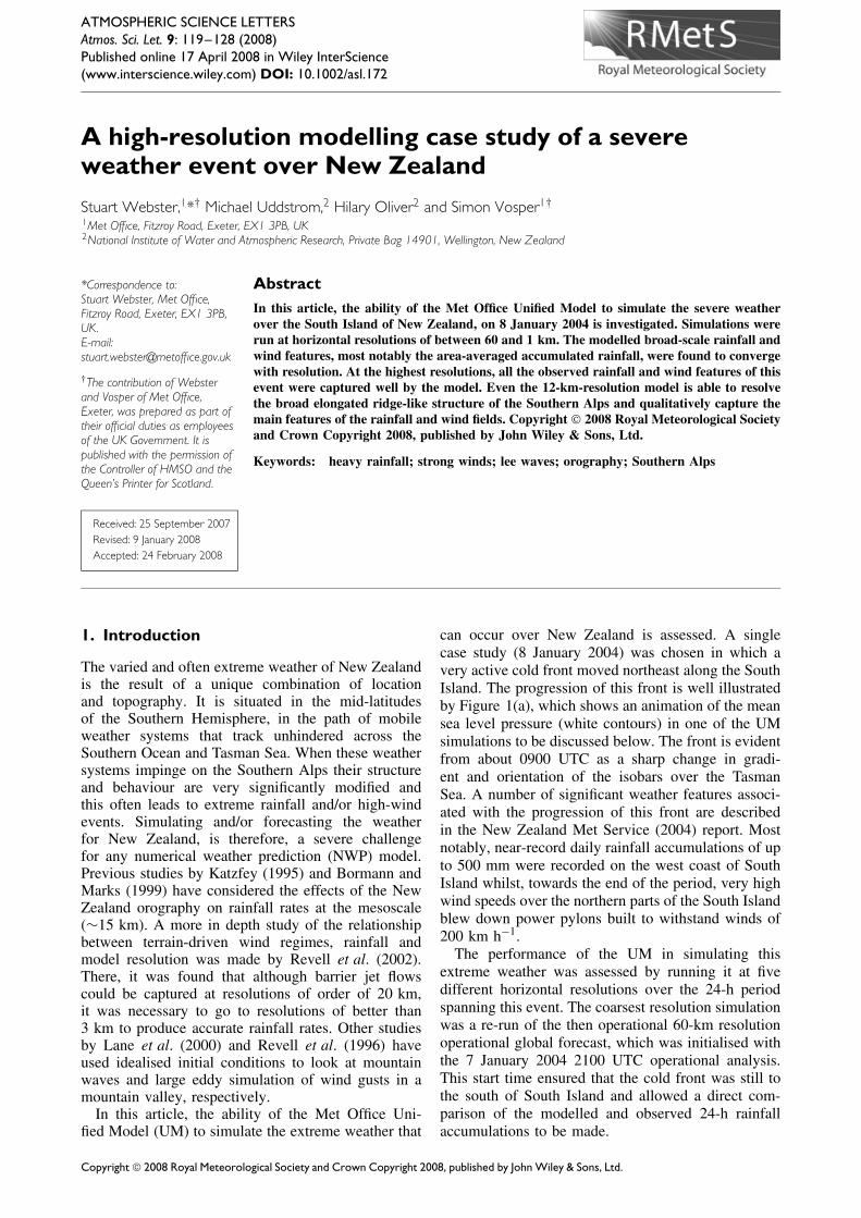
Figure 1. The instantaneous total rainfall rate at 1700 UTCfor the 12-km model (a) and the 2-km model (b). The animatedversion of this figure, which runs from 0200 UTC through to2100 UTC is available in the supplementary materials section.The units are mm h−1 and the ‘Max’ value indicated in the titleof each panel is the maximum instantaneous rate within theregion shown. Also shown in white contours (interval of 1 hPa)in (a) is the instantaneous mean sea level pressure field.

The remaining four limited area simulations weremultiply one-way, nested within the global model athorizontal resolutions of 12, 4, 2 and 1 km. The model

NZLAM-12

NZLAM-4

NZLAM-2

NZLAM-1

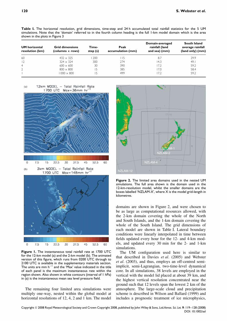
Figure 2. The limited area domains used in the nested UMsimulations. The full area shown is the domain used in the12-km-resolution model, whilst the smaller domains are theboxes labelled ‘NZLAM-X’, where X is the model grid-length inkilometres.

domains are shown in Figure 2, and were chosen tobe as large as computational resources allowed, withthe 2-km domain covering the whole of the Northand South Islands, and the 1-km domain covering thewhole of the South Island. The grid dimensions ofeach model are shown in Table I. Lateral boundaryconditions were linearly interpolated in time betweenfields updated every hour for the 12- and 4-km mod-els, and updated every 30 min for the 2- and 1-kmsimulations.

The UM configuration used here is similar tothat described in Davies et al. (2005) and Websteret al. (2003), and thus, employs an off-centred semi-implicit, semi-Lagrangian, two-time-level dynamicalcore. In all simulations, 38 levels are employed in thevertical with the model lid placed at about 39 km, andthe highest vertical resolution concentrated near theground such that 12 levels span the lowest 2 km of theatmosphere. The large-scale cloud and precipitationscheme is described in Wilson and Ballard (1999) andincludes a prognostic treatment of ice microphysics,

Copyright 2008 Royal Meteorological Society and Crown Copyright 2008, published by John Wiley & Sons, Ltd.Atmos. Sci. Let. 9: 119–128 (2008)DOI: 10.1002/asl

Modelling a severe weather event over New Zealand 121

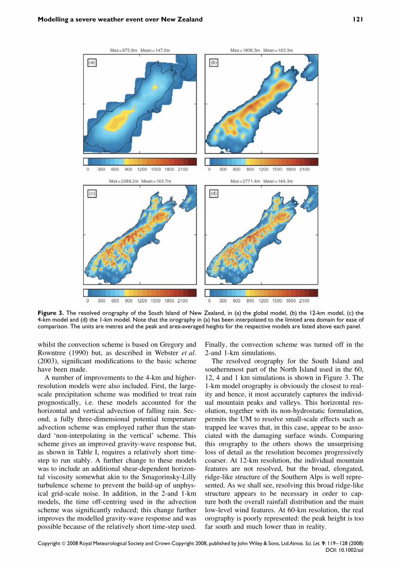
Figure 3. The resolved orography of the South Island of New Zealand, in (a) the global model, (b) the 12-km model, (c) the4-km model and (d) the 1-km model. Note that the orography in (a) has been interpolated to the limited area domain for ease ofcomparison. The units are metres and the peak and area-averaged heights for the respective models are listed above each panel.

whilst the convection scheme is based on Gregory andRowntree (1990) but, as described in Webster et al.(2003), significant modifications to the basic schemehave been made.

A number of improvements to the 4-km and higher-resolution models were also included. First, the large-scale precipitation scheme was modified to treat rainprognostically, i.e. these models accounted for thehorizontal and vertical advection of falling rain. Sec-ond, a fully three-dimensional potential temperatureadvection scheme was employed rather than the stan-dard ‘non-interpolating in the vertical’ scheme. Thisscheme gives an improved gravity-wave response but,as shown in Table I, requires a relatively short time-step to run stably. A further change to these modelswas to include an additional shear-dependent horizon-tal viscosity somewhat akin to the Smagorinsky-Lillyturbulence scheme to prevent the build-up of unphys-ical grid-scale noise. In addition, in the 2-and 1-kmmodels, the time off-centring used in the advectionscheme was significantly reduced; this change furtherimproves the modelled gravity-wave response and waspossible because of the relatively short time-step used.

Finally, the convection scheme was turned off in the2-and 1-km simulations.

The resolved orography for the South Island andsouthernmost part of the North Island used in the 60,12, 4 and 1 km simulations is shown in Figure 3. The1-km model orography is obviously the closest to real-ity and hence, it most accurately captures the individ-ual mountain peaks and valleys. This horizontal res-olution, together with its non-hydrostatic formulation,permits the UM to resolve small-scale effects such astrapped lee waves that, in this case, appear to be asso-ciated with the damaging surface winds. Comparingthis orography to the others shows the unsurprisingloss of detail as the resolution becomes progressivelycoarser. At 12-km resolution, the individual mountainfeatures are not resolved, but the broad, elongated,ridge-like structure of the Southern Alps is well repre-sented. As we shall see, resolving this broad ridge-likestructure appears to be necessary in order to cap-ture both the overall rainfall distribution and the mainlow-level wind features. At 60-km resolution, the realorography is poorly represented: the peak height is toofar south and much lower than in reality.



It is worth reiterating that all our simulations werefree-running, i.e. the only ‘real’ data input is the oper-ational global model analysis at the initial time. There-fore, any differences observed in the higher-resolutionsimulations are due to the improved orography and/orto the improved resolution of the dynamical and phys-ical processes associated with the front.

In summary, our assessment of the UM essentiallyinvolves answering the following two questions:

1. To what extent is the UM capable of capturing theobserved features of this severe weather event?

2. How sensitive is the UM simulation of thesefeatures to the horizontal resolution?

2. Results

2.1. Rainfall

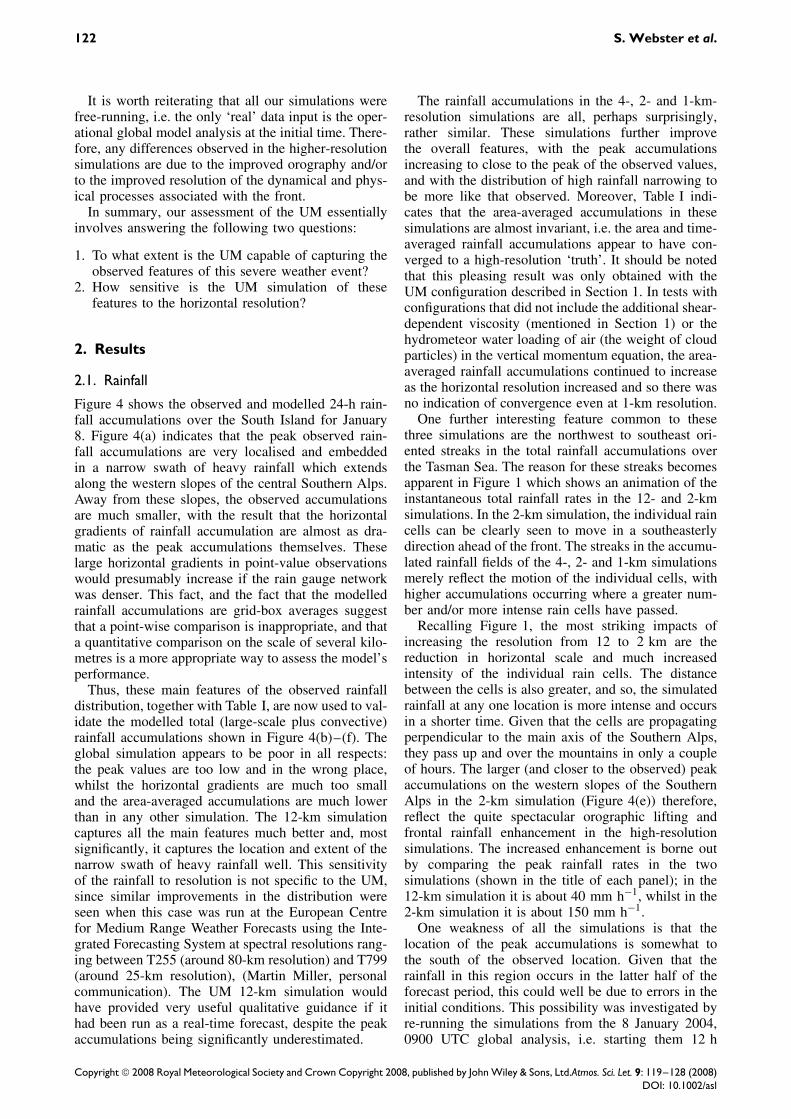
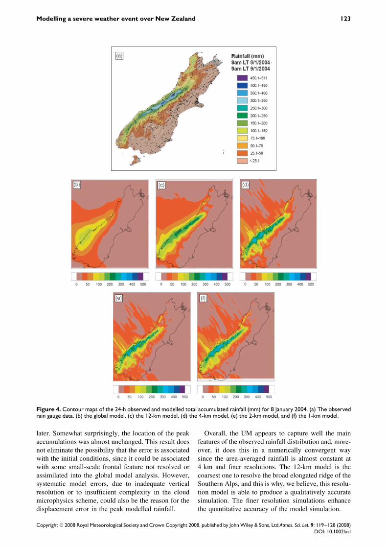
Figure 4 shows the observed and modelled 24-h rain-fall accumulations over the South Island for January8. Figure 4(a) indicates that the peak observed rain-fall accumulations are very localised and embeddedin a narrow swath of heavy rainfall which extendsalong the western slopes of the central Southern Alps.Away from these slopes, the observed accumulationsare much smaller, with the result that the horizontalgradients of rainfall accumulation are almost as dra-matic as the peak accumulations themselves. Theselarge horizontal gradients in point-value observationswould presumably increase if the rain gauge networkwas denser. This fact, and the fact that the modelledrainfall accumulations are grid-box averages suggestthat a point-wise comparison is inappropriate, and thata quantitative comparison on the scale of several kilo-metres is a more appropriate way to assess the model’sperformance.

Thus, these main features of the observed rainfalldistribution, together with Table I, are now used to val-idate the modelled total (large-scale plus convective)rainfall accumulations shown in Figure 4(b)–(f). Theglobal simulation appears to be poor in all respects:the peak values are too low and in the wrong place,whilst the horizontal gradients are much too smalland the area-averaged accumulations are much lowerthan in any other simulation. The 12-km simulationcaptures all the main features much better and, mostsignificantly, it captures the location and extent of thenarrow swath of heavy rainfall well. This sensitivityof the rainfall to resolution is not specific to the UM,since similar improvements in the distribution wereseen when this case was run at the European Centrefor Medium Range Weather Forecasts using the Inte-grated Forecasting System at spectral resolutions rang-ing between T255 (around 80-km resolution) and T799(around 25-km resolution), (Martin Miller, personalcommunication). The UM 12-km simulation wouldhave provided very useful qualitative guidance if ithad been run as a real-time forecast, despite the peakaccumulations being significantly underestimated.

The rainfall accumulations in the 4-, 2- and 1-km-resolution simulations are all, perhaps surprisingly,rather similar. These simulations further improvethe overall features, with the peak accumulationsincreasing to close to the peak of the observed values,and with the distribution of high rainfall narrowing tobe more like that observed. Moreover, Table I indi-cates that the area-averaged accumulations in thesesimulations are almost invariant, i.e. the area and time-averaged rainfall accumulations appear to have con-verged to a high-resolution ‘truth’. It should be notedthat this pleasing result was only obtained with theUM configuration described in Section 1. In tests withconfigurations that did not include the additional shear-dependent viscosity (mentioned in Section 1) or thehydrometeor water loading of air (the weight of cloudparticles) in the vertical momentum equation, the area-averaged rainfall accumulations continued to increaseas the horizontal resolution increased and so there wasno indication of convergence even at 1-km resolution.

One further interesting feature common to thesethree simulations are the northwest to southeast ori-ented streaks in the total rainfall accumulations overthe Tasman Sea. The reason for these streaks becomesapparent in Figure 1 which shows an animation of theinstantaneous total rainfall rates in the 12- and 2-kmsimulations. In the 2-km simulation, the individual raincells can be clearly seen to move in a southeasterlydirection ahead of the front. The streaks in the accumu-lated rainfall fields of the 4-, 2- and 1-km simulationsmerely reflect the motion of the individual cells, withhigher accumulations occurring where a greater num-ber and/or more intense rain cells have passed.

Recalling Figure 1, the most striking impacts ofincreasing the resolution from 12 to 2 km are thereduction in horizontal scale and much increasedintensity of the individual rain cells. The distancebetween the cells is also greater, and so, the simulatedrainfall at any one location is more intense and occursin a shorter time. Given that the cells are propagatingperpendicular to the main axis of the Southern Alps,they pass up and over the mountains in only a coupleof hours. The larger (and closer to the observed) peakaccumulations on the western slopes of the SouthernAlps in the 2-km simulation (Figure 4(e)) therefore,reflect the quite spectacular orographic lifting andfrontal rainfall enhancement in the high-resolutionsimulations. The increased enhancement is borne outby comparing the peak rainfall rates in the twosimulations (shown in the title of each panel); in the12-km simulation it is about 40 mm h−1, whilst in the2-km simulation it is about 150 mm h−1.

One weakness of all the simulations is that thelocation of the peak accumulations is somewhat tothe south of the observed location. Given that therainfall in this region occurs in the latter half of theforecast period, this could well be due to errors in theinitial conditions. This possibility was investigated byre-running the simulations from the 8 January 2004,0900 UTC global analysis, i.e. starting them 12 h



Figure 4. Contour maps of the 24-h observed and modelled total accumulated rainfall (mm) for 8 January 2004. (a) The observedrain gauge data, (b) the global model, (c) the 12-km model, (d) the 4-km model, (e) the 2-km model, and (f) the 1-km model.

later. Somewhat surprisingly, the location of the peakaccumulations was almost unchanged. This result doesnot eliminate the possibility that the error is associatedwith the initial conditions, since it could be associatedwith some small-scale frontal feature not resolved orassimilated into the global model analysis. However,systematic model errors, due to inadequate verticalresolution or to insufficient complexity in the cloudmicrophysics scheme, could also be the reason for thedisplacement error in the peak modelled rainfall.

Overall, the UM appears to capture well the mainfeatures of the observed rainfall distribution and, more-over, it does this in a numerically convergent waysince the area-averaged rainfall is almost constant at4 km and finer resolutions. The 12-km model is thecoarsest one to resolve the broad elongated ridge of theSouthern Alps, and this is why, we believe, this resolu-tion model is able to produce a qualitatively accuratesimulation. The finer resolution simulations enhancethe quantitative accuracy of the model simulation.



2.2. 10-m winds

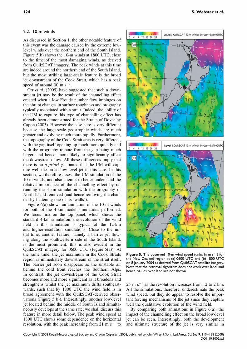
As discussed in Section 1, the other notable feature ofthis event was the damage caused by the extreme low-level winds over the northern end of the South Island.Figure 5(b) shows the 10-m winds at 1800 UTC, closeto the time of the most damaging winds, as derivedfrom QuikSCAT imagery. The peak winds at this timeare indeed around the northern end of the South Island,but the most striking large-scale feature is the broadjet downstream of the Cook Strait, which has a peakspeed of around 30 m s−1.

Orr et al. (2005) have suggested that such a down-stream jet may be the result of the channelling effectcreated when a low Froude number flow impinges onthe abrupt changes in surface roughness and orographytypically associated with a strait. Indeed, the ability ofthe UM to capture this type of channelling effect hasalready been demonstrated for the Straits of Dover byCapon (2003). However the case here is very differentbecause the large-scale geostrophic winds are muchgreater and evolving much more rapidly. Furthermore,the topography of the Cook Strait area is very different,with the gap itself opening up much more quickly andwith the orography remote from the gap being muchlarger, and hence, more likely to significantly affectthe downstream flow. All these differences imply thatthere is no a priori guarantee that the UM will cap-ture well the broad low-level jet in this case. In thissection, we therefore assess the UM simulation of the10-m winds, and also attempt to better understand therelative importance of the channelling effect by re-running the 4-km simulation with the orography ofNorth Island removed (and hence removing the chan-nel by flattening one of its ‘walls’).

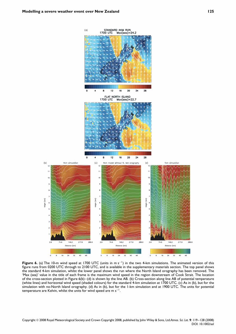
Figure 6(a) shows an animation of the 10-m windsfor both of the 4-km model simulations performed.We focus first on the top panel, which shows thestandard 4-km simulation; the evolution of the windfield in this simulation is typical of the 12-kmand higher-resolution simulations. Close to the ini-tial time, another feature, namely a barrier jet flow-ing along the southwestern side of the South Island,is the most prominent; this is also evident in theQuikSCAT imagery for 0600 UTC (Figure 5(a)). Atthe same time, the jet maximum in the Cook Straitsregion is immediately downstream of the strait itself.The barrier jet soon disappears as the unstable airbehind the cold front reaches the Southern Alps.In contrast, the jet downstream of the Cook Straitbecomes more and more significant as it broadens andstrengthens whilst the jet maximum drifts southeast-wards, such that by 1800 UTC the wind field is inbroad agreement with the QuikSCAT-derived obser-vations (Figure 5(b)). Interestingly, another low-leveljet located behind the middle of South Island simulta-neously develops at the same rate; we shall discuss thisfeature in more detail below. The peak wind speed at1800 UTC shows some dependence on the horizontalresolution, with the peak increasing from 21 m s−1 to

Figure 5. The observed 10-m wind speed (units in m s−1) forthe New Zealand region at (a) 0600 UTC and (b) 1800 UTCon 8 January 2004 as derived from QuikSCAT satellite imagery.Note that the retrieval algorithm does not work over land, andhence, values over land are not shown.

25 m s−1 as the resolution increases from 12 to 2 km.All the simulations, therefore, underestimate the peakwind speed, but they do appear to resolve the impor-tant forcing mechanisms of the jet since they capturewell the qualitative evolution of the wind field.

By comparing both animations in Figure 6(a), theimpact of the channelling effect on the broad low-leveljet can be seen. Interestingly, both the developmentand ultimate structure of the jet is very similar in



Figure 6. (a) The 10-m wind speed at 1700 UTC (units in m s−1) in the two 4-km simulations. The animated version of thisfigure runs from 0200 UTC through to 2100 UTC, and is available in the supplementary materials section. The top panel showsthe standard 4-km simulation, whilst the lower panel shows the run where the North Island orography has been removed. The‘Max (sea)’ value in the title of each frame is the maximum wind speed in the region downstream of Cook Strait. The locationof the cross-section plotted in Figure 6(b)–(d) is shown by the line AB. (b) Cross-section along line AB of potential temperature(white lines) and horizontal wind speed (shaded colours) for the standard 4-km simulation at 1700 UTC. (c) As in (b), but for thesimulation with no-North Island orography. (d) As in (b), but for the 1-km simulation and at 1900 UTC. The units for potentialtemperature are Kelvin, whilst the units for wind speed are m s−1.



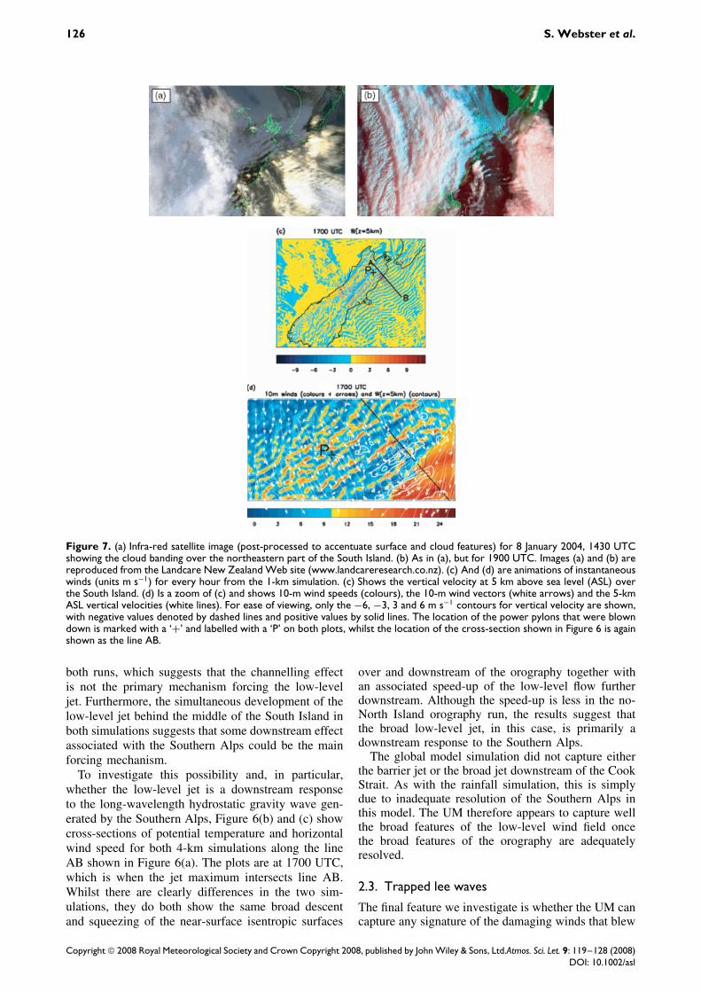
Figure 7. (a) Infra-red satellite image (post-processed to accentuate surface and cloud features) for 8 January 2004, 1430 UTCshowing the cloud banding over the northeastern part of the South Island. (b) As in (a), but for 1900 UTC. Images (a) and (b) arereproduced from the Landcare New Zealand Web site (www.landcareresearch.co.nz). (c) And (d) are animations of instantaneouswinds (units m s−1) for every hour from the 1-km simulation. (c) Shows the vertical velocity at 5 km above sea level (ASL) overthe South Island. (d) Is a zoom of (c) and shows 10-m wind speeds (colours), the 10-m wind vectors (white arrows) and the 5-kmASL vertical velocities (white lines). For ease of viewing, only the −6, −3, 3 and 6 m s−1 contours for vertical velocity are shown,with negative values denoted by dashed lines and positive values by solid lines. The location of the power pylons that were blowndown is marked with a ‘+’ and labelled with a ‘P’ on both plots, whilst the location of the cross-section shown in Figure 6 is againshown as the line AB.

both runs, which suggests that the channelling effectis not the primary mechanism forcing the low-leveljet. Furthermore, the simultaneous development of thelow-level jet behind the middle of the South Island inboth simulations suggests that some downstream effectassociated with the Southern Alps could be the mainforcing mechanism.

To investigate this possibility and, in particular,whether the low-level jet is a downstream responseto the long-wavelength hydrostatic gravity wave gen-erated by the Southern Alps, Figure 6(b) and (c) showcross-sections of potential temperature and horizontalwind speed for both 4-km simulations along the lineAB shown in Figure 6(a). The plots are at 1700 UTC,which is when the jet maximum intersects line AB.Whilst there are clearly differences in the two sim-ulations, they do both show the same broad descentand squeezing of the near-surface isentropic surfaces

over and downstream of the orography together withan associated speed-up of the low-level flow furtherdownstream. Although the speed-up is less in the no-North Island orography run, the results suggest thatthe broad low-level jet, in this case, is primarily adownstream response to the Southern Alps.

The global model simulation did not capture eitherthe barrier jet or the broad jet downstream of the CookStrait. As with the rainfall simulation, this is simplydue to inadequate resolution of the Southern Alps inthis model. The UM therefore appears to capture wellthe broad features of the low-level wind field oncethe broad features of the orography are adequatelyresolved.

2.3. Trapped lee waves

The final feature we investigate is whether the UM cancapture any signature of the damaging winds that blew



down the power pylons mentioned in Section 1. Thepylons in question were located close to Molesworth,adjacent to the Kaikoura mountain range. Figure 7(a)shows satellite cloud imagery from 1430 UTC, closeto the time that the pylons toppled over, whilstFigure 7(b) shows the cloud imagery at 1900 UTC.A series of parallel cloud bands close to where thepylons were blown down is evident at 1430 UTC, andthis train of clouds has extended downstream and outover the sea by 1900 UTC. These cloud bands indi-cate the presence of trapped lee waves, with the cloudbands lying in the crest of the waves. Beneath thecrest of these waves turbulent rotors and sub-rotorsmay produce extreme wind gusts at low levels (Doyleand Durran, 2007), even though the mean surfaceflow is reduced or even reversed. In the trough of thewaves, the mean surface flow is increased which coulddirectly lead to the damaging surface winds. Therefore,in this section, we assess whether the UM can capturethe trapped lee waves and associated changes in meansurface winds.

Given the short (15–20 km) wavelength of thetrapped lee wave train, only the 1-km simulationcan reasonably be expected to capture any significantsignal of the damaging low-level winds. Figure 7(c)shows an animation of the vertical velocity at 5 kmabove sea level from the 1-km simulation (as thepotential temperature contours in Figure 6(d) show,this is close to the level of the maximum ampli-tude). Significant gravity wave activity is seen todevelop over and downstream of most of the South-ern Alps. The waves are, for the most part quasi-stationary although they show significant eastwardpropagation as the front approaches and the mean flowspeed increases. This non-stationarity is consistentwith the behaviour discussed by Vosper and Worthing-ton (2002), who examined how non-zero phase speedsare related to the acceleration of the upstream flow.

A direct comparison of the modelled lee wave train(Figure 7(c)) along line AB at 1900 UTC with the leewave train evident in the satellite imagery at this time(Figure 7(b)) suggests that the trapped lee waves arewell simulated, since the wavelength and downstreamextent compare favourably. Peak vertical velocitiesat this time are of the order of 10 m s−1 whichare consistent with the wave activity in this regionbeing quite exceptional. The corresponding heightsection along AB (Figure 6(d)) indicates how muchadditional complexity of the flow field is captured atthis resolution compared to that at 4-km resolution(Figure 6(b)). Furthermore, it is evident that the wavesare weaker near the surface than aloft, suggesting thatthey reside in a slightly elevated duct. The heightof this duct is likely to be very difficult to simulatecorrectly (e.g. being highly sensitive to the boundarylayer scheme). Since the impact of the ducting is toreduce the surface wind variations, simulating thesevariations correctly is likely to be very difficult.

Nonetheless, the issue of whether there is anysignature of the low-level winds that blew down

the power pylons in the 1-km simulation is furtherinvestigated in Figure 7(d), which shows an animationof the 10-m winds and the vertical velocities at5 km above sea level for the Molesworth region.The low-level winds at the location of the pylonsare relatively weak throughout the course of thesimulation. However, the large horizontal variations inwind speed that develop in this region are consistentwith the significant wave activity already noted. Theweak winds imply that the location of the pylons couldbe beneath a wave crest, and so the damaging windscould be due to the turbulence associated with a near-surface rotor. Equally, the phase of modelled gravitywaves generated by high mountains is well known tobe extremely difficult to get right even for isolatedtopography (e.g. Smith and Broad, 2003), so phaseerrors in this complex wave field are perhaps to beexpected. In reality, the pylons may well have beensituated underneath a wave trough with associatedstrong mean surface winds. Either way, the large leewave activity in this region is consistent with a highprobability of damaging near-surface winds in andaround the location of the pylons.

3. Summary

In this article, we have evaluated the forecastingcapability of the UM over New Zealand. A casestudy was chosen in which several different extremeweather features were observed, with the intentionof investigating whether the UM could capture thesefeatures and, if so, how sensitive the simulation wasto the horizontal resolution.

The UM was found to capture each of the extremefeatures well, once the model resolution was suffi-cient to resolve the key relevant aspect of the orog-raphy adequately. The rainfall, the broad low-leveljet downstream of the Cook Strait and the barrier jetwere all well captured by the 12-km model – this wasthe coarsest resolution that first captured the elon-gated ridge-like structure of the Southern Alps. Ingeneral, as we would hope, the UM was found tobe numerically convergent, with the higher-resolutionsimulations providing additional detail and quanti-tative improvements, but the broader-scale featuresbeing largely unchanged compared to those at thecoarser resolutions. The one feature that required a 1-km resolution to be adequately captured was the non-hydrostatic trapped lee wave response; this was unsur-prising given the small horizontal scale of these waves.

Acknowledgements

The authors would like to thank Stuart Moore and AdamClayton for providing the Unified Model initial data andancillary fields. Thanks are also due to the Joint Centre forMesoscale Meteorology at the University of Reading, and inparticular to Richard Forbes and Humphrey Lean, for providingupdated versions of the high-resolution model configuration,and to Andrew Tait (NIWA) who provided the surface rain



accumulation analysis. Thanks also to Martin Miller (ECMWF)for running this case study using the Integrated ForecastingSystem. This work was largely funded by the New ZealandFoundation for Research, Science and Technology, undercontract C01X0401.

References

Bormann N, Marks CJ. 1999. Mesoscale rainfall forecasts over NewZealand during SALPEX96: characterization and sensitivity studies.Monthly Weather Review 127: 2880–2894.

Capon RA. 2003. Wind speed up in the Dover Straits with theMet Office New Dynamics Model. Meteorological Applications 10:229–237.

Davies T, Cullen MJP, Malcolm AJ, Mawson MH, Staniforth A,White AA, Wood N. 2005. A new dynamical core for the MetOffice’s global and regional modelling of the atmosphere. QuarterlyJournal of the Royal Meteorological Society 131: 1759–1782.

Doyle JD, Durran DR. 2007. Rotor and sub-rotor dynamics in the leeof three dimensional terrain. Journal of the Atmospheric Sciences 64:4202–4221.

Gregory D, Rowntree PR. 1990. A mass flux convection schemewith representation of cloud ensemble characteristics and stability-dependent closure. Monthly Weather Review 118: 1483–1506.

Katzfey JJ. 1995. Simulation of extreme New Zealand precipitationevents. Part I.: sensitivity to orography and resolution. MonthlyWeather Review 123: 737–754.

Lane TP, Reeder MJ, Morton BR, Clark TL. 2000. Observations andModelling of mountain waves over the Southern Alps of New

Zealand. Quarterly Journal of the Royal Meteorological Society 126:2765–2788.

New Zealand Met Service. 2004. Heavy rain on West Coast; severenortherly gales in central districts 9 January 2004, Available on-line at http://www.metservice.co.nz/default/index.php?static=2003summer1.

Orr A, Hunt JCR, Capon RA, Sommeria J, Cresswell D, Owinoh A.2005. Coriolis effects on wind jets and cloudiness along coasts.Weather 60: 291–299.

Revell MJ, Purnell DK, Lauren MK. 1996. Requirements for large-eddy simulation of surface wind gusts in a mountain valley.Boundary-Layer Meteorology 80: 333–353.

Revell MJ, Copeland JH, Larsen HR, Wratt DS. 2002. Barrier jetsaround the Southern Alps of New Zealand and their potential toenhance alpine rainfall. Atmospheric Research 61: 277–298.

Smith SA, Broad AS. 2003. Horizontal and temporal variability ofmountain waves over Mont Blanc. Quarterly Journal of the RoyalMeteorological Society 129: 2195–2216.

Vosper SB, Worthington RM. 2002. VHF radar measurements andmodel simulations of mountain waves over Wales. Quarterly Journalof the Royal Meteorological Society 128: 185–204.

Webster S, Brown AR, Jones CP, Cameron DR. 2003. Improvementsto the Representation of orography in the Met Office UnifiedModel. Quarterly Journal of the Royal Meteorological Society 129:1989–2010.

Wilson DR, Ballard SP. 1999. A microphysically based precipitationscheme for the Meteorological Office Unified Model. QuarterlyJournal of the Royal Meteorological Society 125: 1607–1636.


a high-resolution modelling case study of a severe weather event over new zealand

Documents