a hierarchical model for association rule mining of ...tyler/pubs/mccormick_recsys.pdf · a...

Submitted to the Annals of Applied StatisticsarXiv: math.PR/0000000

A HIERARCHICAL MODEL FOR ASSOCIATION RULEMINING OF SEQUENTIAL EVENTS: AN APPROACH TO

AUTOMATED MEDICAL SYMPTOM PREDICTION

By Tyler H. McCormick∗, Cynthia Rudin

†and David Madigan

∗

Columbia University∗ and Massachusetts Institute of Technology†

In many healthcare settings, patients visit healthcare profession-als periodically and report multiple medical conditions, or symptoms,at each encounter. We propose a statistical modeling technique, calledthe Hierarchical Association Rule Model (HARM), that predicts apatient’s possible future symptoms given the patient’s current andpast history of reported symptoms. The core of our technique is aBayesian hierarchical model for selecting predictive association rules(such as “symptom 1 and symptom 2 → symptom 3”) from a largeset of candidate rules. Because this method “borrows strength” usingthe symptoms of many similar patients, it is able to provide predic-tions specialized to any given patient, even when little informationabout the patient’s history of symptoms is available.

1. Introduction. The emergence of large-scale medical record databasespresents exciting opportunities for data-based personalized medicine. Predic-tion lies at the heart of personalized medicine and in this paper we proposea statistical model for predicting patient-level sequences of medical symp-toms. We draw on new approaches for predicting the next event within a“current sequence,” given a “sequence database” of past event sequences(Rudin et al., 2010). Specifically we propose the Hierarchical AssociationRule Mining Model (HARM) that generates a set of association rules suchas dyspepsia and epigastric pain→ heartburn, indicating that dyspepsia andepigastric pain are commonly followed by heartburn. HARM produces aranked list of these association rules. Both patients and caregivers can usethe rules to guide medical decisions. Built-in explanations represent a par-ticular advantage of the association rule framework—the rule predicts heart-burn because the patient has had dyspepsia and epigastric pain.

In our setup, we assume that each patient visits a healthcare providerperiodically. At each encounter, the provider records time-stamped medicalsymptoms experienced since the previous encounter. In this context, weaddress several prediction problems such as:

AMS 2000 subject classifications: Primary 60K35, 60K35; secondary 60K35Keywords and phrases: Association rule mining, healthcare surveillance, hierarchical

model, machine learning

1

http://www.imstat.org/aoas/

http://arxiv.org/abs/math.PR/0000000

2 T. H. MCCORMICK ET AL.

• Given data from a sequence of past encounters, predict the next symp-tom that a patient will experience.

• Given basic demographic information, predict the first symptom thata patient will report.

• Given partial data from an encounter (and possibly prior encounters)predict the next symptom.

Though medical databases often contain records from thousands or evenmillions of patients, most patients experience only a handful of the massiveset of potential symptoms. This patient-level sparsity presents a challengefor predictive modeling. Our hierarchical modeling approach attempts toaddress this challenge by borrowing strength across patients.

Applications of association rules usually do not usually concern super-vised learning problems (though there exist some exceptions, e.g. Velosoet al., 2008). The sequential event prediction problem is a supervised learn-ing problem, that as far as we know, has been formalized only here and byRudin et al. (2010). DuMouchel and Pregibon (2001) presented a Bayesiananalysis of association rules. Their approach, however, does not apply in ourcontext because of the sequential nature of our data.

The experiments this paper presents indicate that HARM outperformsseveral baseline approaches including a standard “maximum confidence,minimum support threshold” technique used in association rule mining, andalso a non-hierarchical version of our Bayesian method (from Rudin et al.,2010) that ranks rules using “adjusted confidence.”

More generally, HARM yields a prediction algorithm for sequential datathat can potentially be used for a wide variety of applications beyond symp-tom prediction. For instance, the algorithm can be directly used as a rec-ommender system (for instance, for vendors such as Netflix, amazon.com,or online grocery stores such as Fresh Direct and Peapod). It can be usedto predict the next move in a video game in order to design a more inter-esting game, or it can be used to predict the winners at each round of atournament (e.g., the winners of games in a football season). All of theseapplications possess the same basic structure as the symptom predictionproblem: a database consisting of sequences of events, where each event isassociated to an individual entity (medical patient, customer, football team).As future events unfold in a new sequence, our goal is to predict the nextevent.

In Section 2 we provide basic definitions and present our model. In Sec-tion 3 we evaluate the predictive performance of HARM, along with severalbaselines through experiments on clinical trial data. Section 4 provides re-lated work, and Section 5 provides a discussion and offers potential exten-

AHIERARCHICALMODEL FOR ASSOCIATION RULEMININGOF SEQUENTIAL EVENTS3

sions.

2. Method. This work presents a new approach to association rule min-ing by determining the “interestingness” of rules using a particular (hierar-chical) Bayesian estimate of the probability of exhibiting symptom b, givena set of current symptoms, a. We will first discuss association rule miningand its connection to Bayesian shrinkage estimators. Then we will presentour hierarchical method for providing personalized symptom predictions.

2.1. Definitions. An association rule in our context is an implicationa → b where the left side is a subset of symptoms that the patient has expe-rienced, and b is a single symptom that the patient has not yet experiencedsince the last encounter. Ultimately, we would like to rank rules in terms of“interestingness” or relevance for a particular patient at a given time. Usingthis ranking, we make predictions of subsequent conditions. Two commondetermining factors of the “interestingness” of a rule are the “confidence”and “support” of the rule (Agrawal, Imielinski and Swami, 1993; Piatetsky-Shapiro, 1991).

The confidence of a rule a → b for a patient is the empirical probability:

Conf(a → b) :=Number of times symptoms a and b were experienced

Number of times symptoms a were experienced

:= P (b|a).

The support of set a is:

Support(a) := Number of times symptoms a were experienced

∝ P (a),

where P (a) is the empirical proportion of times that symptoms a were expe-rienced. When a patient has experienced a particular set of symptoms onlya few times, a new single observation can dramatically alter the confidenceP (b|a) for many rules. This problem occurs commonly in our clinical trialdata, where most patients have reported fewer than 10 total symptoms. Thevast majority of rule mining algorithms address this issue with a minimumsupport threshold to exclude rare rules, and the remaining rules are eval-uated for interestingness (reviews of interestingness measures include thoseof Tan, Kumar and Srivastava, 2002; Geng and Hamilton, 2007). The defini-tion of interestingness is often heuristic, and is often not even a meaningfulestimate of P (b|a).

It is well-known that problems arise from using a minimum supportthreshold. For instance, consider the collection of rules meeting the min-imum support threshold condition. Within this collection, the confidence


alone should not be used to rank rules: among rules with similar confi-dence, the rules with larger support should be preferred. More importantly,“nuggets,” which are rules with low support but very high confidence, areoften excluded by the threshold. This is problematic, for instance, when asymptom that occurs rarely is strongly linked with another rare symptom,it is essential not to exclude the rules characterizing these symptoms. In ourdata, the distribution of symptoms has a long tail, where the vast majorityof events happen rarely: out of 1800 possible symptoms, 1400 occur less than10 times. These 1400 symptoms are precisely the ones in danger of beingexcluded by a minimum support threshold.

Our work avoids problems with the minimum support threshold by rank-ing rules with a shrinkage estimator of P (b|a). These estimators directlyincorporate the support of the rule. One example of such an estimator is the“adjusted confidence” (Rudin et al., 2010):

AdjConf(a → b,K):=Number of times symptoms a and b were experienced

Number of times symptoms a were experienced +K.

The effect of the penalty term K is to pull low-support rules towards thebottom of the list; any rule achieving a high adjusted confidence must over-come this pull through either a high enough support or a high confidence.Using the adjusted confidence avoids the problems discussed earlier: “inter-estingness” is closely related to the conditional probability P (b|a), rules areextremely interpretable, among rules with equal confidence the higher sup-port rules are preferred, and there is no strict minimum support threshold.

In this work, we extend the adjusted confidence model in an importantrespect, in that our method shares information across similar patients tobetter estimate the conditional probabilities. The adjusted confidence is aparticular Bayesian estimate of the confidence. Assuming a Beta prior dis-tribution for the confidence, the posterior mean is:

P (b|a) := α+#(a ∪ b)

α+ β +#a,

where #x is the support of symptom x, and α and β denote the parametersof the (conjugate) beta prior distribution. Our model allows the parametersof the binomial to be chosen differently for each patient and also for eachrule. This means that our model can determine, for instance, whether aparticular patient is more likely to repeat a symptom that has occurredonly once, and also whether a particular symptom is more likely to repeatthan another.

We note that our approach makes no explicit attempt to infer causalrelationships between symptoms. The observed associations may in fact arise


from common prior causes such as other symptoms or drugs. Thus a rulesuch as dyspepsia → heartburn does not necessarily imply that successfultreatment of dyspepsia will change the probability of heartburn. Rather thegoal is to accurately predict heartburn in order to facilitate effective medicalmanagement.

2.2. Hierarchical Association Rule Model (HARM). For a patient i anda given rule, r, say we observe yir co-occurrences (support for lhs ∩ rhs) innir relevant previous encounters (support for lhs). We model the numberof co-occurrences as Binomial(nir, pir) and then model pir hierarchically toshare information across groups of similar individuals. Define M as a I ×Dmatrix of static observable characteristics for a total of I individuals andD observable characteristics, where we assume D > 1 (otherwise we revertback to a model with a rule-wise adjustment). Each row of M correspondsto a patient and each column to a particular characteristic. We define thecolumns of M to be indicators of particular patient categories (gender, orage between 30 and 40, for example), though they could be continuous inother applications. Let Mi denote the ith row of the matrix M. We modelthe probability for the ith individual and the rth rule pir as coming from abeta distribution with parameters πir and τi. We then define πir throughthe regression model πir = exp(M�

iβr + γi) where βr defines a vector ofregression coefficients for rule r and γi is an individual-specific random effect.More formally, we propose the following model:

yir ∼ Binomial(nir, pir)

pir ∼ Beta(πir, τi)

πir = exp(M�iβr + γi).

Under this model,

E(pir|yir, nir) =yir + πir

nir + πir + τi,

which is a more flexible form of adjusted confidence. This expectation alsoproduces non-zero probabilities for a rule even if nir is 0 (patient i has neverreported the symptoms on the left hand side of r before). The fixed effectregression component,M�

iβr, adjusts πir based on the patient characteristicsin the M matrix. For example, if the entries of M represented only gender,then the regression model with intercept βr,0 would be βr,0+βr,11male where1male is one for male respondents and zero for females. Being male, therefore,has a multiplicative effect of eβr,1 on πir. In this example, the M�

iβr valueis the same for all males, encouraging similar individuals to have similar


values of πir. For each rule r, we will use a common prior on all coefficientsin βr; this imposes a hierarchical structure, and has the effect of regularizingcoefficients associated with rare characteristics.

The πir’s allow rare but important “nuggets” to be recommended. Evenacross multiple patient encounters, many symptoms occur very infrequently.In some cases these symptoms may still be highly associated with certainother conditions. For instance, compared to some symptoms, migraines arerelatively rare. Patients who have migraines however typically also experi-ence nausea. A minimum support threshold algorithm might easily excludethis rule if migraines if a patient hasn’t experienced many migraines in thepast. This is especially likely for patients who have few encounters. In ourmodel, the πir term balances the regularization imposed by τi to, for certainindividuals, increase the ranking of rules with high confidence but low sup-port. The τi term reduces the probability associated with rules that haveappeared few times in the data (low support), with the same effect as thepenalty term (K) in the adjusted confidence. Unlike the cross-validationor heuristic strategies suggested in Rudin et al. (2010), we estimate τi aspart of an underlying statistical model. Within a given rule, we assume τifor every individual comes from the same distribution. This imposes addi-tional structure across individuals, increasing stability for individuals withfew observations.

It remains now to describe the precise prior structure on the regressionparameters and hyperparameters. We assign Gaussian priors with mean 0and variance σ2

τ to the τ on the log scale. Since any given patient is unlikely toexperience a specific medical condition, the majority of probabilities are closeto zero. Giving τi a prior with mean zero improves stability by discouragingexcessive penalties. We assign all elements βr,d of vectors βr a commonGaussian prior on the log scale with mean µβ and variance σ2

β. We alsoassume each γi comes from a Gaussian distribution on the log scale withcommon mean µγ and variance σ2

γ . Each individual has their own γi term,which permits flexibility among individuals; however, all of the γi terms comefrom the same distribution, which induces dependence between individuals.We assume diffuse uniform priors on the hyperparameters µτ , σ2

τ , µβ, andσ2β. Denote Y as the matrix of yir values, N as the matrix of nir values, and

β as the collection of β1, . . . ,βR. The prior assumptions yield the following


posterior:

p,π, τ,β|Y,N,M ∝I�

i=1

R�

r=1

pyir+πirir (1− pir)

nir−yir+τi

×R�

r=1

D�

d=1

Normal(log(βr,d)|µβ,σ2β)

×I�

i=1

Normal(log(γi)|µγ ,σ2γ)Normal(log(τi)|0,σ2

τ ).

HARM produces draws from the (approximate) posterior distribution foreach probability. In the context of symptom prediction, these probabilitiesare of interest and we analyze our estimates of their full posterior distribu-tions in Section 3.2. To rank association rules for the purpose of prediction,however, we need a single estimate for each probability (rather than a fulldistribution), which we chose as the posterior mode. We carry out our com-putations using a Gibbs sampling algorithm, provided in Figure 1.

2.3. Online updating. Given a batch of data, HARM makes predictionsbased on the posterior distributions of pir. Since the posterior is not availablein closed form, predictions using HARM requires iterating the algorithm inFigure 1 to convergence. The next time the patient visits the physician, pircould be updated by again iterating the algorithm in Figure 1 to conver-gence. In some applications new data continue arrive frequently, making itimpractical to compute approximate posterior distributions using the algo-rithm in Figure 1 for each new encounter. In this section we provide anonline updating scheme which incorporates new patient data after an initialbatch of encounters has already been processed.

Beginning with an initial batch of data, we run the algorithm in Figure 1to obtain τi and πir, which are defined to be posterior mean of the estimateddistributions for τi and πir. Given that up to encounter e − 1, we have

observed y(e−1)ir and n(e−1)

ir , we are presented with new observations that

have counts y(newobs.)ir and n(newobs.)ir so that y(e)ir = y(e−1)

ir + y(newobs.)ir and

n(e)ir = n(e−1)

ir + n(newobs.)ir . In order to update the probability estimates to

reflect our total current data, y(e)ir , n(e)ir , we will use the following relationship:

P (pir|y(e)ir , n(e)ir , τi, πir) ∝ P (y(newobs.)ir |n(newobs.)

ir , pir)

×P (pir|y(e−1)ir , n(e−1)

ir , τi, πir).

The expression P (pir|y(e−1)ir , n(e−1)

ir , τi, πir) is the posterior up to encountere − 1 and has a beta distribution. The likelihood of the new observations,


For a suitably initialized chain, at step v:

1. Update pir from the conjugate Beta distribution given π, τ,Y,N,M.

2. Update τi using a Metropolis step with proposal τ∗i where

log(τ∗i ) ∼ N(τ (v−1)

i , (scale of jumping dist)).

3. For each rule, update the vector βr using a Metropolis step with

log(β∗r) ∼ N(β(v−1)

r , (scale of jumping dist)).

4. Update γi using a Metropolis step with

log(γ∗i ) ∼ N(γ(v−1)

i , (scale of jumping dist)).

5. Update µβ ∼ N(µβ,σ2β) where

µβ =�

1D +R

� R�

r=1

D�

d=1

βr,d.

6. Update σ2β ∼ Inv-χ2(d− 1, σ2

β) where

σ2β =

�1

D +R

� R�

r=1

D�

d=1

(βr,d − µβ)2.

7. Update σ2τ ∼ Inv-χ2(I − 1, σ2

τ ) where σ2τ = 1

I

�I

i=1(τi − µτ )

2.

8. Update µγ ∼ N(µγ ,σ2γ) where µγ = 1

I

�I

i=1γi.

9. Update σ2γ ∼ Inv-χ2(I − 1, σ2

γ) where σ2γ = 1

I

�I

i=1(γi − µγ)

2.

Fig 1. Gibbs sampling algorithm for hierarchical bayesian association rule mining forsequential event prediction (HARM).


P (y(newobs.)ir |n(newobs.)ir , pir), is binomial. Conjugacy implies that the updated

posterior also has a beta distribution. In order to update the probability esti-mates for our hierarchical model, we use the expectation of this distribution,that is

E(pir|y(e)ir , n(e)ir , τi, πir) =

y(e−1)ir + ynewobs.ir + πir

n(e−1)ir + nnewobs.

ir + πir + τi.

3. Application to repeated patient encounters. We present resultsof HARM, with the online updating scheme in Section 2.3, on co-prescribingdata from a large clinical trial. These data are from around 42,000 patientencounters from about 2,300 patients, all at least 40 years old. The matrix ofobservable characteristics encodes the basic demographic information: gen-der, age group (40-49, etc.), ethnicity. For each patient we have a record ofeach medication prescribed and the symptom/chief complaint (back pain,asthma, etc) that warranted the prescription. We chose to predict patientcomplaints rather than prescriptions since there are often multiple prescrib-ing options (medications) for the same complaint. Some patients had pre-existing conditions that continued throughout the trial. For these patients,we include these pre-existing conditions in the patient’s list of symptomsat each encounter. Other patients have recurrent conditions for which wewould like to predict the occurrences. If a patient reports the same condi-tion more than once during the same thirty day period we only consider thefirst occurrence of the condition at the first report. If the patient reports thecondition once and then again more than thirty days later, we consider thistwo separate incidents.

As covariates, we used age, gender, race and drug/placebo. We fit ageusing a series of indicator variables corresponding to four groups (40-49,50-59, 60-69, 70+).

Our experiments consider only the marginal probabilities (support) andprobabilities conditional on one previous symptom. Thus, the left hand sideof each rule contains either 0 items or 1 item.

In Section 3.1 we present experimental results to compare the predictiveperformance of our model to other rule mining algorithms for this type ofproblem. In Section 3.2 we use the probability estimates from the model todemonstrate its ability to find new associations; in particular, we find asso-ciations that are present in medical literature but that may not be obviousby considering only the raw data.

3.1. Predictive performance. We selected a sample of patients by assign-ing each patient a random draw from a Bernoulli distribution with success


probability selected to give a sample of patients on average around 200. Foreach patient we drew uniformly an integer ti between 0 and the numberof encounters for that patient. We ordered the encounters chronologicallyand used encounters 1 through ti as our training set and the remainingencounters as the test set. Through this approach, the training set encom-passes the complete set of encounters for some patients (“fully observed”),includes no encounters for others (“new patients”), and a partial encounterhistory of the majority of the test patients (“partially observed patients”).We believe this to be a reasonable approximation of the context where thistype of method would be applied, with some patients having already beenobserved several times and other new patients entering the system for thefirst time. We evaluated HARM’s predictive performance using the top 50most frequently reported conditions; these conditions represent 60% of allconditions reported.

The algorithm was used to iteratively predict the condition revealed ateach encounter. For each selected patient, starting with their first test en-counter, and prior to that encounters’ condition being revealed, the algo-rithm made a prediction of c possible conditions, where c = 3. Note thatto predict the very first condition for a given patient when there are noprevious encounters, the recommendations come from posterior modes ofthe coefficients estimated from the training set. The algorithm earned onepoint if it recommended the current condition before it was revealed, andno points otherwise. Then, yir and nir were updated to include the currentcondition. This process was repeated for the patient’s remaining encounters.We then moved to the next patient and repeated the procedure.

The total score of the algorithm for a given patient was computed asthe total number of points earned for that patient divided by the totalnumber of conditions experienced by the patient. The total score of thealgorithm is the average of the scores for the individual patients. Thus, thetotal score is the average proportion of correct predictions per patient. Werepeated this entire process (beginning with selecting patients) 500 times andrecorded the distribution over the 500 scores. We compared the performanceof HARM (using the same scoring system) against an algorithm that ranksrules by adjusted confidence, for several values of K. We also compared withthe “max confidence minimum support threshold” algorithm for differentvalues of the support threshold θ, where rules with support below θ areexcluded and the remaining rules are ranked by confidence. For both ofthese algorithms, no information across patients is able to be used.

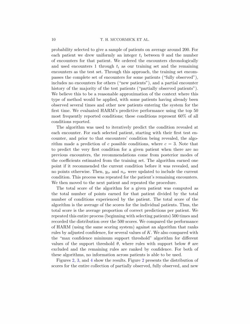
Figures 2, 3, and 4 show the results. Figure 2 presents the distribution ofscores for the entire collection of partially observed, fully observed, and new


●●●●

●

●

●

●●●

●

●

●●●●

●●●●●●●●●●

●●●●●

●

●●●

●●

●

HAR

MC

onf.

Adj.

k=.2

5Ad

j. k=

.5Ad

j. k=

1Ad

j. k

=2Th

resh

.=2

Thre

sh.=

3

0.1

0.2

0.3

0.4

All patientsPr

opor

tion

of c

orre

ct p

redi

ctio

ns

Fig 2. Predictive performance for all patients. Each boxplot represents the distributionof scores over 500 runs. These plots include data from both partially observed and newpatients.


●

●

●●●●

●

●●●●

●

●

●

●●●

●

●●

●

●●●●

●

●●

●

●

●

●●

●●●

●

●

HAR

MC

onf.

Adj.

k=.2

5Ad

j. k=

.5Ad

j. k=

1Ad

j. k

=2Th

resh

.=2

Thre

sh.=

3

0.1

0.2

0.3

0.4

0.5

Partially observed patients

Prop

ortio

n of

cor

rect

pre

dict

ions

Fig 3. Predictive performance for partially observed patients. These are patients for whichthere are training encounters.


●

●

●●●●●●●●● ●

●●

●

●●●●●●●●●●●● ●●

●●●●●●●●

●●●●●●

●

●

●

●●●

HAR

MC

onf.

Adj.

k=.2

5Ad

j. k=

.5Ad

j. k=

1Ad

j. k

=2Th

resh

.=2

Thre

sh.=

3

0.0

0.1

0.2

0.3

0.4

New patients

Prop

ortio

n of

cor

rect

pre

dict

ions

Fig 4. Predictive performance for new patients.


patients. Paired t-tests comparing the mean proportion of correct predictionsfrom HARM to each of the alternatives had p-values for a significant differ-ence in our favor less than 10−15. In other words, HARM has statisticallysuperior performance over all K and θ; i.e., better performance than eitherof the two algorithms even if their parameters K and θ had been tuned tothe best possible value. For all four values of K for the adjusted confidence,performance was slightly better than for the plain confidence (K = 0). The“max confidence minimum support threshold” algorithm (which is a stan-dard approach to association rule mining problems) performed poorly forminimum support thresholds of 2 and 3. This poor performance is likelydue to the sparse information we have for each patient. Setting a minimumsupport threshold as low as even two eliminates many potential candidaterules from consideration.

The main advantage of our model is that it shares information across pa-tients in the training set. This means that in early stages where the observedyir and nir are small, it may still be possible to obtain reasonably accurateprobability estimates, since when patients are new, our recommendationsdepend heavily on the behavior of previously observed similar patients. Weconsider the predictive performance of HARM with respect to partially ob-served (Figure 3) and new (Figure 4) patients. Though our method overallhas a higher frequency of correct predictions than the other algorithms inboth cases, the advantage is more pronounced for new patients; in caseswhere there is no data for each patient, there is a large advantage to sharinginformation.

3.2. Association mining. The conditional probability estimates from ourmodel are also a way of mining a large and highly dependent set of associa-tions.

Ethnicity, high cholesterol or hypertension → myocardial infarction: Figure5 plot (a) shows the distribution of posterior median propensity for myocar-dial infarction (heart attack) given two conditions previously reported asrisk factors for myocardial infarction: high cholesterol and hypertension (seeKukline, Yoon and Keenan, 2010, for a recent review). Each bar in the fig-ure corresponds to the set of respondents in a specified ethnic group. ForCaucasians, we typically estimate a higher probability of myocardial infarc-tion in patients who have previously had high cholesterol. In African Ameri-cans / Hispanics and Asian patients, however, we estimate a generally higherprobability for patients who have reported hypertension. This distinctiondemonstrates the flexibility of our method in combining information across


a) HARM b) Confidence

Fig 5. Propensity of myocardial infarction in patients who have reported high cholesterolor hypertension using HARM (plot (a)) and (unadjusted) confidence (plot (b)). For eachdemographic group, high cholesterol (HC) is on the left and hypertension (Hy) is on theright. Thick lines represent the middle half of the posterior median propensities for re-spondents in the indicated demographic group. Outer lines represent the middle 90% anddots represent the mean. The vast majority of patients did not experience a myocardialinfarction, which places the middle 90% of the distribution in plot (b) approximately atzero.

respondents who are observably similar. Some other specific characteristicsof the estimated distributions vary with ethnicity, for instance, the propen-sity distribution for Caucasians who have had high cholesterol has a muchlonger tail than those of the other ethnic groups.

As a comparison, we also included the same plot using (unadjusted) con-fidence, in Figure 5 (b). The black dots are the mean across all the patients,which are not uniformly at zero because there were some cases of myocar-dial infarction and hypertension or high cholesterol. The colored, smallerdots represent the rest of the distribution (quartiles), which appear to be atzero in plot (b) since the vast majority of patients did not have a myocardialinfarction at all, so even fewer had a myocardial infarction after reportinghypertension or high cholesterol.

Age, high cholesterol or hypertension, treatment or placebo →myocardial infarction: Since our data come from a clinical trial, we also in-cluded an indicator of treatment vs. placebo condition in the hierarchicalregression component of HARM. Figures 6 and 7 display the posterior medi-ans of propensity of myocardial infarction for respondents separated by ageand treatment condition. Figure 6 considers patients who have reported hy-pertension, Figure 7 considers patients who have reported high cholesterol.In both Figure 6 and Figure 7, it appears that the propensity of myocar-



Fig 6. Propensity of myocardial infarction in patients who have reported hypertension, es-timated by HARM (plot (a)) and (unadjusted) confidence (plot (b)). For each demographicgroup, the placebo (P) is on the left and the treatment medication (T) is on the right. Thicklines represent the middle half of the posterior median propensities for respondents in theindicated demographic group. Outer lines represent the middle 90% and dots represent themean. Overall the propensity is higher for individuals who take the study medication thatthose who do not.


Fig 7. Propensity of myocardial infarction in patients who have reported high cholesterol,estimated by HARM (plot (a)) and (unadjusted) confidence (plot (b)). For each demo-graphic group, the placebo (P) is on the left and the treatment medication (T) is on theright. Thick lines represent the middle half of the posterior median propensities for respon-dents in the indicated demographic group. Outer lines represent the middle 90% and dotsrepresent the mean.

dial infarction predicted by HARM is greatest for individuals between 50and 70, with the association again being stronger for high cholesterol thanhypertension.

For both individuals with either high cholesterol or hypertension, use


of the treatment medication was associated with increased propensity ofmyocardial infarction. This effect is present across nearly every age category.The distinction is perhaps most clear among patients in their fifties in bothFigure 6 and Figure 7. The treatment product in this trial has been linkedto increased risk of myocardial infarction in numerous other studies. Theproduct was eventually withdrawn from the market by the manufacturerbecause of its association with myocardial infarctions.

The structure imposed by our hierarchical model gives positive probabil-ities even when no data are present in a given category; in several of thecategories, we observed no instances of a myocardial infarction, so estimatesusing only the data cannot differentiate between the categories in terms ofrisk for myocardial infarction, as demonstrated by Figures 6(b) and 7(b).

4. Related Works. As far as we know, the line of work by Davis et al.(2009) is the first to use an approach from recommender systems to pre-dict medical symptoms, though in a completely different way than ours; itis based on vector similarity, in the same way as Breese, Heckerman andKadie (1998a) (also see references in Davis et al. (2009) for background oncollaborative filtering).

Three relevant works on Bayesian hierarchical modeling and recommendersystems are those of DuMouchel and Pregibon (2001, “D&P”), Breese, Heck-erman and Kadie (1998b), and Condliff, Lewis and Madigan (1999). D&Pdeal with the identification of interesting itemsets (rather than identificationof rules). Specifically, they model the ratio of observed itemset frequencies tobaseline frequencies computed under a particular model for independence.Neither Breese et al. nor Condliff et al. aim to model repeat purchases (re-curring symptoms). Breese et al. uses Bayesian methods to cluster users,and also suggests a Bayesian network. Condliff, Lewis and Madigan (1999)present a hierarchical Bayesian approach to collaborative filtering that “bor-rows strength” across users.

5. Conclusion and Future Work. We have presented a hierarchicalmodel for ranking association rules for sequential event prediction. The se-quential nature of the data is captured through rules that are sensitive totime order, that is, a → b indicates symptoms a are followed by symptomsb. HARM uses information from observably similar individuals to augmentthe (often sparse) data on a particular individual; this is how HARM isable to estimate probabilities P (b|a) before symptoms a have ever been re-ported. In the absence of data, hierarchical modeling provides structure. Asmore data become available, the influence of the modeling choices fade asgreater weight is placed on the data. The sequential prediction approach is


especially well suited to medical symptom prediction, where experiencingtwo symptoms in succession may have different clinical implications thanexperiencing either symptom in isolation.

collaborative nature of medical symptoms make the sequential predidtionThere are several possible directions for future work. One possibility is to

investigate whether expanding the set of rules has an influence on predictionaccuracy. In the case that the set of rules is too large, it may be importantto develop parsimonious representations of these associations, potentiallythrough a method similar to model-based clustering (Fraley and Raftery,2002). Another direction is to incorporate higher-order dependence, alongthe line of work by Berchtold and Raftery (2002). A third potential futuredirection is to design a more sophisticated online updating procedure thanthe one in Section 2.3. It may be possible to design a procedure that directlyupdates the hyperparameters as more data arrive.

Acknowledgements. Tyler McCormick is supported by a Google PhDFellowship in Statistics.

References.

Agrawal, R., Imielinski, T. and Swami, A. (1993). Mining association rules between setsof items in large databases. In SIGMOD ’93: Proceedings of the 1993 ACM SIGMODinternational conference on Management of data 207–216. ACM, New York, NY, USA.

Berchtold, A. and Raftery, A. E. (2002). The Mixture Transition Distribution Modelfor High-Order Markov Chains and Non-Gaussian Time Series. Statistical Science 17pp. 328-356.

Breese, J. S., Heckerman, D. and Kadie, C. (1998a). Empirical Analysis of PredictiveAlgorithms for Collaborative Filtering. 43–52. Morgan Kaufmann.

Breese, J. S., Heckerman, D. and Kadie, C. M. (1998b). Empirical Analysis of Pre-dictive Algorithms for Collaborative Filtering. In Proc. Uncertainty in Artificial Intel-ligence 43-52.

Condliff, M. K., Lewis, D. D. andMadigan, D. (1999). Bayesian Mixed-Effects Modelsfor Recommender Systems. In ACM SIGIR 99 Workshop on Recommender Systems:Algorithms and Evaluation.

Davis, D. A., Chawla, N. V., Christakis, N. A. and Barabsi, A.-L. (2009). Timeto CARE: a collaborative engine for practical disease prediction. Data Mining andKnowledge Discovery 20 388-415.

DuMouchel, W. and Pregibon, D. (2001). Empirical Bayes screening for multi-itemassociations. In Proc. ACM SIGKDD international conference on Knowledge discoveryand data mining 67–76.

Fraley, C. and Raftery, A. E. (2002). Model-Based Clustering, Discriminant Analysis,and Density Estimation. Journal of the American Statistical Association 97 611-631.

Gelman, A., Carlin, J., Stern, H. and Rubin, D. (2003). Bayesian Data Analysis, 2ed. Chapman and Hall/CRC.

Geng, L. and Hamilton, H. J. (2007). Choosing the Right Lens: Finding What is Inter-esting in Data Mining. In Quality Measures in Data Mining 3-24. Springer.


Kukline, E., Yoon, P. W. and Keenan, N. L. (2010). Prevalence of Coronary HeartDisease Risk Factors and Screening for High Cholesterol Levels Among Young Adults,United States, 1999-2006. Annals of Family Medicine 8 327-333.

Piatetsky-Shapiro, G. (1991). Discovery, analysis and presentation of strong rules. InKnowledge Discovery in Databases (G. Piatetsky-Shapiro and W. J. Frawley, eds.) 229–248. AAAI Press.

Rudin, C., Salleb-Aouissi, A., Kogan, E. and Madigan, D. (2010). A Framework forSupervised Learning with Association Rules. Submitted.

Tan, P. N., Kumar, V. and Srivastava, J. (2002). Selecting the right interestingnessmeasure for association patterns. In KDD ’02: Proc. Eighth ACM SIGKDD interna-tional conference on Knowledge discovery and data mining.

Veloso, A. A., Almeida, H. M., Goncalves, M. A. and Jr., W. M. (2008). Learningto rank at query-time using association rules. In SIGIR ’08: Proceedings of the 31st an-nual international ACM SIGIR conference on Research and development in informationretrieval 267–274. ACM, New York, NY, USA.

Address of the First and Third authors

Department of Statistics

Columbia University

1255 Amsterdam Ave. New York, NY 10027, USA

E-mail: [email protected]@stat.columbia.edu

Address of the Second author

MIT Sloan School of Management, E62-576

Massachusetts Institute of Technology

Cambridge, MA 02139, USA

E-mail: [email protected]

mailto:[email protected]



a hierarchical model for association rule mining of ...tyler/pubs/mccormick_recsys.pdf · a...

Documents