A Hierarchical Matching of Deformable Shapes

Pedro FelzenszwalbDepartment of Computer Science

University of Chicago

Joint work with Joshua Schwartz

Shape-based recognition

• Humans can recognize many objects based on shape alone.

• Fundamental cue for many object categories.

• Classical approach for recognizing rigid objects.

• Invariant to photometric variation.

Comparing and matching shapes

• Related problems

- Measuring the similarity between shapes.

- Finding a set of correspondences between shapes.

- Finding a shape similar to a model in an image.

≈

Elastic matching

• Measure amount of bending and stretching necessary to turn one curve into another [Basri et al 95], [Sebastian et al 03].

- Similar to computing edit distance between strings.

- Efficient dynamic programming algorithms.

- Can capture some but not all important shape aspects.

Can turn these into each other without much bending anywhere.

Similar objects with completely different local boundary properties.

A1

A2

B1

B2

q2

q1

q3p3

p2

p1

• Compose matchings between subcurves to get longer matchings.

- Different kind of dynamic programming.

• Cost of combination depends on:

- Cost of matchings being combined.

- Arrangement of endpoints.

Our approach: compositional method

For long matchings the endpoints are far away and we capture global geometric properties.

b a

ce

dg

fh

i

g | e,c i | d,bh | c,df | a,e

d | c,be | a,c

c | a,b

Shape-tree

• Shape-tree of curve from a to b:

- Select midpoint c, store relative location c | a,b.

- Left child is a shape-tree of sub-curve from a to c.

- Right child is a shape-tree of sub-curve from c to b.

b a

ce

dg

fh

i

g | e,c i | d,bh | c,df | a,e

d | c,be | a,c

c | a,b

Shape-tree

• Invariant to similarity transformation.

• Sub-tree is shape-tree of sub-curve.

• Given placement for a,b we can reconstruct the curve.

• Bottom nodes captures local curvature.

• Top nodes capture curvature of sub-sampled curve.

Relative locations

• Bookstein coordinates for representing B | A,C.

• There exists a unique similarity transformation T taking:

- A to (-1/2,0)

- C to (1/2,0)

• Look at T(B).

(-1/2,0) (1/2,0)

A

B

C

A

B

C

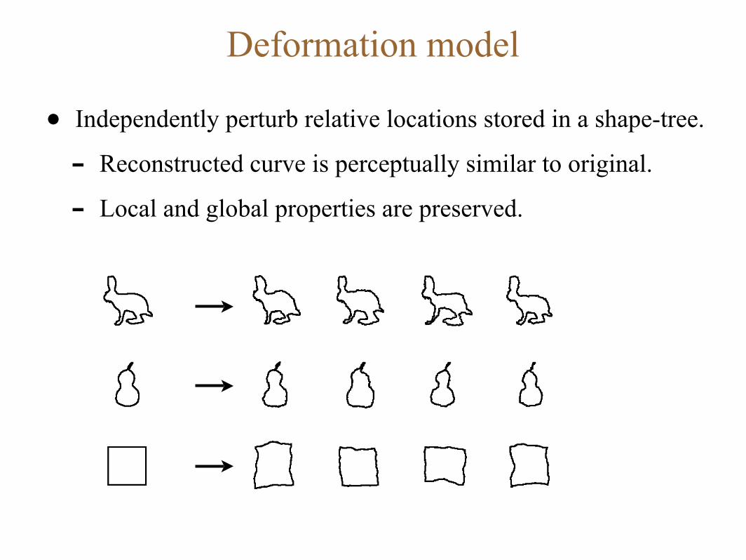
Deformation model

• Independently perturb relative locations stored in a shape-tree.

- Reconstructed curve is perceptually similar to original.

- Local and global properties are preserved.

Distance between curves

• Given curves A and B.

• Can’t compare shape-trees for A and B built separately.

• Search over shape-trees for A and B looking for similar pair.

- Can be done in O(n3m3) time using DP (n = |A|, m = |B|).

• Our current approach:

- Fix shape-tree for A and look for map from points in A to

points in B that doesn’t deform the shape-tree much.

- Efficient O(nm3) DP algorithm.

Matching open curves

• Curves: A = (a1, ..., an) and B = (b1, ..., bm).

• Assume a1 → b1 and an → bm.

• Shape-tree defines midpoint ai dividing A into A1 and A2.

• Search over corresponding point bj dividing B.

ψ(A,B) = minbj

(ψ(A1, B1) + ψ(A2, B2) +λ ∗ dif((ai|a1, an), (bj |b1, bm))

)

is similarity between A and B.ψ

measures difference in relative locations.dif

is a scaling factor.λ

Dynamic programming

• Let v be node in shape-tree of A.

- Corresponds to subcurve A’.

• Table T(v):

- T(v)[i][j] is cost of matching A’ to (bi, ..., bj).

- T(v) can be computed using T(u) and T(w) where u and w are children of v in shape-tree.

• O(n) tables, O(m2) entries per table, O(m) to compute entry.

- O(nm3) algorithm.

• Generalization can cut off sub-trees to allow for missing parts.

• Can also handle closed curves...

Recognition results - swedish leaves

Nearest neighbor classification

Shape-tree 96.28

Inner distance 94.13

Shape context 88.12

15 species

75 examples per species

(25 training, 50 test)

Recognition results - MPEG7

Bullseye score

Shape-tree 87.70

Hier. procrustes 86.35

Inner distance 85.40

Curve edit 78.14

Shape context 76.51

Example categories:

70 categories

20 shapes per category

Cluttered images

(1) input (2) edges

(3) contours (4) detection

model

b

a

M C

p

q

Matching to cluttered images

• M: model (closed curve).

• C: curves in image.

• P: endpoints of curves in C.

• Match([a,b], [p,q]): matching of subcurve of M from a to bto subset of C with a → p and b → q.

Matching to cluttered images

• Use DP to match each curve in C to every subcurve of M.

- Generate a set of initial matchings Match([a,b], [p,q]).

- Running time is linear on total length of image contours.

• Define gap matching Match([a,b], [p,q]) from every subcurve of M to every pair of anchor points in the image.

- Cost depends on length of [a,b].

• Stitch partial matchings together to form longer matchings.

- Using compositional rule.

- Second phase of DP.

Compositional rule

m = (q+r)/2

Match([a,b], [p,q]) = w1

Match([b,c], [r,s]) = w2

Match([a,c], [p,s]) = w1 + w2 + dif((b|a,c), (m|p,s))

If ||q-r|| < T can compose Match([a,b], [p,q]) and Match([b,c], [r,s])

b

a

cM C

s

r

p

q

Example compositions

• Composing

- Match([c,d], [r,s]), Match([d,e], [t,u]).

- Get Match([c,e], [r,u]).

- Match([a,b], [p,q]) with gap matching Match([b,c], [q,r]).

- Get matching Match([a,c], [p,r]).

- ...

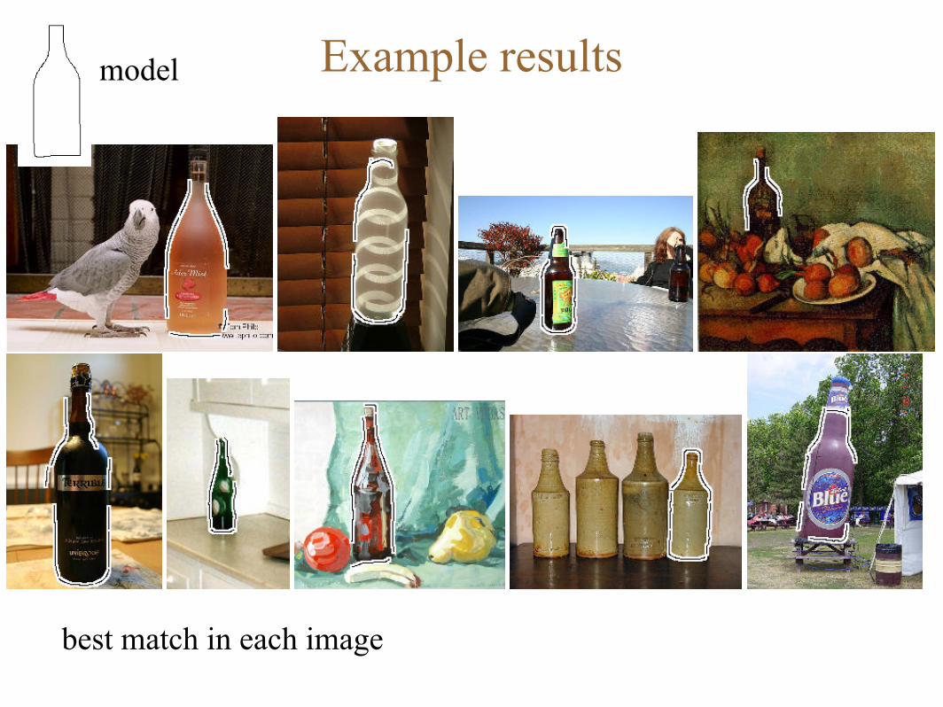
Example results

Figure 11. Some example results of matching a bottle to images in the ETHZ dataset. Only the best match in each image is shown. Most

of the gaps in each matching are due to missing edges.

Figure 12. Some example results of matching a swan to images in the ETHZ dataset. Only the best match in each image is shown. The

third image on the top shows a mistake, due to missing edges on the swan and extra edges on the water.

8

best match in each image

model

More resultsFigure 11. Some example results of matching a bottle to images in the ETHZ dataset. Only the best match in each image is shown. Most

of the gaps in each matching are due to missing edges.

Figure 12. Some example results of matching a swan to images in the ETHZ dataset. Only the best match in each image is shown. The

third image on the top shows a mistake, due to missing edges on the swan and extra edges on the water.

8

best match in each image

model

Object detection

Part-based models

• Sub-trees usually represent fairly generic curves.

• We can share sub-trees among different models.

- Leads to a notion of parts.

- Useful for bottom-up matching.

• We can generalize shape-tree models using grammars.

- Allows for models to share parts.

- Parts can share sub-parts.

- Objects can have variable structure.

Hierarchical curve models (HCM)

• Underlying PCFG defying the “syntactic” structure of objects.

- Single terminal l corresponding to line segment.

- Productions:

• X → l

• X → YZ

• X(a,b) is curve of type X from a to b.

• Geometry of curve is defined by its structure and conditional distributions over midpoint choice.

- For each rule r = X → YZ we have Pr(c | a,b).

• To generate a curve of type X from a to b,

- Pick production r = X → YZ.

- Pick midpoint c from Pr(c | a,b).

- Generate curve of type Y from a to c and Z from c to b.

• Get a new stochastic grammar:

- Nonterminals X(a,b) and terminals l(a,b).

- Sentences are polygonal chains: l(a1,a2) l(a2,a3) ... l(an-1,an).

- P(X(a,b) → Y(a,c)Z(c,b)) = P(X → YZ) Pr(c | a,b).

- P(X(a,b) → l(a,b)) = P(X → l).

Examples

• Shape-tree deformation model is HCM with fixed structure.

- Underlying grammar has one non-terminal and production for each node in shape-tree.

- Always generates the same structure.

- Pr(c | a,b) is parametric model defined by midpoint location.

• L(a,b) generates an “almost straight curve” from a to b:

- L(a,b) ➝ L(a,c) L(c,b) where c ~ (a+b)/2

- L(a,b) ➝ l(a,b)

- Recursive model with a single non-terminal.

• These are two extremes...

Current and future work...

• Relationship to wavelets.

• Learning HCMs from example shapes.

• Using HCMs for parsing images.

• ...

random shapes