a heuristic prover for real inequalities
TRANSCRIPT
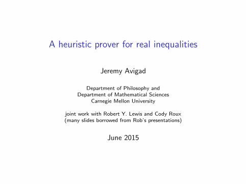
A heuristic prover for real inequalities
Jeremy Avigad
Department of Philosophy andDepartment of Mathematical Sciences
Carnegie Mellon University
joint work with Robert Y. Lewis and Cody Roux(many slides borrowed from Rob’s presentations)
June 2015

Computer support for mathematics
Two variables:
• level of user interaction
• strength of correctness guarantees
Both are continua.
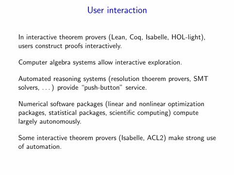
User interaction
In interactive theorem provers (Lean, Coq, Isabelle, HOL-light),users construct proofs interactively.
Computer algebra systems allow interactive exploration.
Automated reasoning systems (resolution thoerem provers, SMTsolvers, . . . ) provide “push-button” service.
Numerical software packages (linear and nonlinear optimizationpackages, statistical packages, scientific computing) computelargely autonomously.
Some interactive theorem provers (Isabelle, ACL2) make strong useof automation.
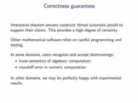
Correctness guarantees
Interactive theorem provers construct formal axiomatic proofs tosupport their claims. This provides a high degree of certainty.
Other mathematical software relies on careful programming andtesting.
In some domains, users recognize and accept shortcomings:
• loose semantics of algebraic computation
• roundoff error in numeric computation
In other domains, we may be perfectly happy with experimentalresults.

Automation and Correctness
unverified verified
automated
automatedtheorem provers,
numeric andsymbolic
computation
verified theoremprovers, verified
computation
interactive
computer algebrasystems,
“notebook”environments
interactivetheorem proving

Polya
Polya provides automated methods to establish real-valuedinequalities.
Desiderata:
• Automatically verify inequalities that come up in interactivetheorem proving.
• Construct formal axiomatic proofs backing them up.

Inequalities
Mathematics is largely about measurement, and comparingquantities.
Show Γ ` s ≤ t.
• pure mathematics: analysis, number theory, combinatorics,geometry, probability
• applied mathematics: engineering, statistics, data analysis,modeling and prediction, . . .
One can use symbolic or numeric methods.

Linear inequalities
Consider entailments of the form
t1 ≥ 0, t2 ≥ 0, . . . , tn ≥ 0⇒ s > 0
The entailment is valid iff the constraints
t1 ≥ 0, t2 ≥ 0, . . . , tn ≥ 0,−s ≥ 0
are infeasible.
Linear programming methods can handle hundreds of thousands ofvariables and constraints.
The methods are exact, and it is not hard to extract certificates /proofs.
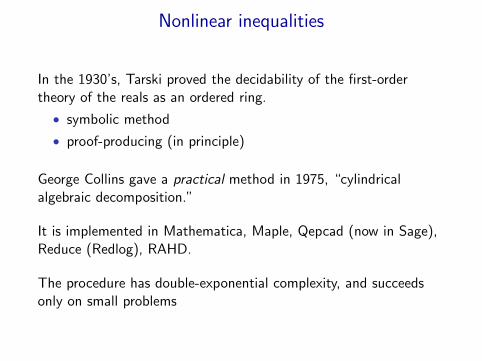
Nonlinear inequalities
In the 1930’s, Tarski proved the decidability of the first-ordertheory of the reals as an ordered ring.
• symbolic method
• proof-producing (in principle)
George Collins gave a practical method in 1975, “cylindricalalgebraic decomposition.”
It is implemented in Mathematica, Maple, Qepcad (now in Sage),Reduce (Redlog), RAHD.
The procedure has double-exponential complexity, and succeedsonly on small problems

Numerical methods
There are a variety of numerical methods, including:
• Interval methods, and interval constraint propagation.
• Convex programming techniques.
• Optimization, stochastic methods.

Combination methods
Paulson’s MetiTarski:
• uses a resolution theorem prover to guide search.
• replaces transcendental function by bounding rationalfunctions.
• uses RCF back ends (Qepcad, Z3, Mathematica)
SMT solvers combine linear integer / real arithmetic methods,real-closed fields.
Parillo has used semidefinite programming methods to verifypositivity of RCF expressions.

Verified numerical methods
Thomas Hales’ proof of the Kepler conjecture required verifyinghundred of inequalities. Most were of the form:
∀~x , ~x ∈ D ⇒ f (~x) > 0 ∨ . . . ∨ f (~x) > 0
where D is a rectangular box.
Solovyev’s 2012 thesis (under Hales’ supervision) developedmethods for handling these.
• Use interval methods based on Taylor series approximations.
• Also use interval methods to detect monotonicity alongcoordinates.

Polya
Polya is a heuristic theorem prover for real-valued inequalities.
• It is designed as automated support for interactive theoremproving.
• It is (will be) proof producing.
• It uses heuristic, symbolic methods.

An example
Consider the following implication:
0 < x < y , u < v
=⇒2u + exp(1 + x + x4) < 2v + exp(1 + y + y4)
• This inference is not contained in linear arithmetic or realclosed fields.
• This inference is tight: symbolic or numeric approximationsare not useful. (Also, the domain is unbounded.)
• But, the inference is completely straightforward.

Backchaining
One idea is a apply rules like u < v ,w ≤ x ⇒ u + w < v + xbackwards.
But we can prove a + b + c < d + e by proving
• a < d , c ≤ e
• a + c ≤ e, b < d
• a + c + 5 ≤ e, b − 5 < d ,
• . . .

Another example
Here’s an inequality that comes up in Shapiro’s presentation of theSelberg proof of the prime number theorem.
Assuming
n ≤ (K/2)x
0 < C
0 < ε < 1
we have (1 +
ε
3(C + 3)
)· n < Kx
Decision procedures for real closed fields seem the wrong way togo.
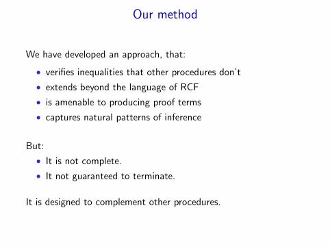
Our method
We have developed an approach, that:
• verifies inequalities that other procedures don’t
• extends beyond the language of RCF
• is amenable to producing proof terms
• captures natural patterns of inference
But:
• It is not complete.
• It not guaranteed to terminate.
It is designed to complement other procedures.

Overview
The main ideas:
• Use forward reasoning (guided by the structure of theproblem).
• Show “hypotheses⇒ conclusion” by negating the conclusionand deriving a contradiction.
• As much as possible, put terms in canonical “normal forms,”e.g. to recognize that 3(x + y) is a multiple of 2y + 2x .
• Derive relationships between “terms of interest,” includingsubterms of the original problem.
• Different modules contribute bits of information, based ontheir expertise.

Language
Our system verifies inequalities between real variables using:
• Operations + and ·• Multiplication and exponentiation by rational constants
• Arbitrary function symbols (described by axioms)
• Relations < and =
All functions are assumed to be total. 1/0,√−1, etc. exist, but no
assumptions are made about their values.

Terms and normal forms
The inequality
15 < 3(3y + 5x + 4xy)2f (u + v)−1
is expressed canonically as
1︸︷︷︸t0
≤ 5 · ( x︸︷︷︸t1
+3
5· y︸︷︷︸
t2
+4
5· xy︸︷︷︸t3=t1t2
)2f ( u︸︷︷︸t4
+ v︸︷︷︸t5
)−1

Terms and normal forms
The inequality
15 < 3(3y + 5x + 4xy)2f (u + v)−1
is expressed canonically as
1︸︷︷︸t0
≤ 5 · ( x︸︷︷︸t1
+3
5· y︸︷︷︸
t2
+4
5· xy︸︷︷︸t3=t1t2︸ ︷︷ ︸
t6=t1+35t2+
45t3
)2f ( u︸︷︷︸t4
+ v︸︷︷︸t5︸ ︷︷ ︸
t7=t4+t5
)−1

Terms and normal forms
The inequality
15 < 3(3y + 5x + 4xy)2f (u + v)−1
is expressed canonically as
1︸︷︷︸t0
≤ 5 · ( x︸︷︷︸t1
+3
5· y︸︷︷︸
t2
+4
5· xy︸︷︷︸t3=t1t2︸ ︷︷ ︸
t6=t1+35t2+
45t3
)2 f ( u︸︷︷︸t4
+ v︸︷︷︸t5︸ ︷︷ ︸
t7=t4+t5︸ ︷︷ ︸t8=f (t7)
)−1

Terms and normal forms
The inequality
15 < 3(3y + 5x + 4xy)2f (u + v)−1
is expressed canonically as
1︸︷︷︸t0
≤ 5 · ( x︸︷︷︸t1
+3
5· y︸︷︷︸
t2
+4
5· xy︸︷︷︸t3=t1t2︸ ︷︷ ︸
t6=t1+35t2+
45t3
)2 f ( u︸︷︷︸t4
+ v︸︷︷︸t5︸ ︷︷ ︸
t7=t4+t5︸ ︷︷ ︸t8=f (t7)
)−1
︸ ︷︷ ︸t9=t26 t
−18

Terms and normal forms
The inequality
15 < 3(3y + 5x + 4xy)2f (u + v)−1
is expressed canonically as
1︸︷︷︸t0
≤ 5 · ( x︸︷︷︸t1
+3
5· y︸︷︷︸
t2
+4
5· xy︸︷︷︸t3=t1t2︸ ︷︷ ︸
t6=t1+35t2+
45t3
)2 f ( u︸︷︷︸t4
+ v︸︷︷︸t5︸ ︷︷ ︸
t7=t4+t5︸ ︷︷ ︸t8=f (t7)
)−1
︸ ︷︷ ︸t9=t26 t
−18︸ ︷︷ ︸
t0≤5t9

Modules and the “blackboard”
Any comparison between canonical terms can be expressed asti ./ 0 or ti ./ c · tj , where ./ ∈ {=, 6=, <,≤, >,≥}.
All modules are assumed to “understand” these relationships.
A central database, the blackboard, stores term definitions andcomparisons of this form.
Modules use this information to learn and assert new comparisons.
The procedure has succeeded in verifying an implication whenmodules assert contradictory information.

Computational structure
BlackboardStores definitions and
comparisons
Additive ModuleDerives comparisons using
additive definitions
Multiplicative ModuleDerives comparisons using
multiplicative definitions
Axiom Instantiation ModuleDerives comparisons using universal
axioms
Exp/Log ModuleDerives comparisons and
axioms involving exp and log
Min/MaxModule
Derives comparisons
involving min and
max
CongruenceClosure Module
Enforces proper
interpretation of
functions
Absolute ValueModule
Derives comparisons and
axioms involving abs
nth Root ModuleDerives comparisons and axioms
about fractional exponents

Arithmetical modules
Modules for additive and multiplicative arithmetic work together tosolve arithmetical problems.
They “saturate” the blackboard with the strongest derivableatomic comparisons.
We use two techniques for this:
• Fourier-Motzkin variable elimination
• a geometric projection method

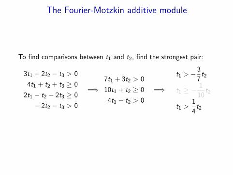
The Fourier-Motzkin additive module
The Fourier-Motzkin algorithm is a quantifier eliminationprocedure for 〈R, 0,+, <〉.
Given additive equations {ti =∑
j cj · tkj} and atomic comparisons{ti ./ c · tj} and {ti ./ 0}:
• For each pair i , j , eliminate all variables except ti and tj .
• Add the strictest remaining comparisons to the blackboard.

The Fourier-Motzkin additive module
To find comparisons between t1 and t2, eliminate t3:
3t1 + 2t2 − t3 > 0
4t1 + t2 + t3 ≥ 0
2t1 − t2 − 2t3 ≥ 0
− 2t2 − t3 > 0
=⇒7t1 + 3t2 > 0
10t1 + t2 ≥ 0
4t1 − t2 > 0
=⇒
t1 >−3
7t2
t1 ≥ −1
10t2
t1 >1
4t2
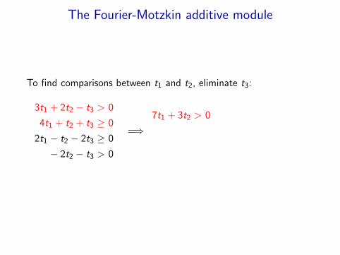
The Fourier-Motzkin additive module
To find comparisons between t1 and t2, eliminate t3:
3t1 + 2t2 − t3 > 0
4t1 + t2 + t3 ≥ 0
2t1 − t2 − 2t3 ≥ 0
− 2t2 − t3 > 0
=⇒7t1 + 3t2 > 0
10t1 + t2 ≥ 0
4t1 − t2 > 0
=⇒
t1 >−3
7t2
t1 ≥ −1
10t2
t1 >1
4t2

The Fourier-Motzkin additive module
To find comparisons between t1 and t2, eliminate t3:
3t1 + 2t2 − t3 > 0
4t1 + t2 + t3 ≥ 0
2t1 − t2 − 2t3 ≥ 0
− 2t2 − t3 > 0
=⇒7t1 + 3t2 > 0
10t1 + t2 ≥ 0
4t1 − t2 > 0
=⇒
t1 >−3
7t2
t1 ≥ −1
10t2
t1 >1
4t2

The Fourier-Motzkin additive module
To find comparisons between t1 and t2, eliminate t3:
3t1 + 2t2 − t3 > 0
4t1 + t2 + t3 ≥ 0
2t1 − t2 − 2t3 ≥ 0
− 2t2 − t3 > 0
=⇒7t1 + 3t2 > 0
10t1 + t2 ≥ 0
4t1 − t2 > 0
=⇒
t1 >−3
7t2
t1 ≥ −1
10t2
t1 >1
4t2

The Fourier-Motzkin additive module
To find comparisons between t1 and t2, find the strongest pair:
3t1 + 2t2 − t3 > 0
4t1 + t2 + t3 ≥ 0
2t1 − t2 − 2t3 ≥ 0
− 2t2 − t3 > 0
=⇒7t1 + 3t2 > 0
10t1 + t2 ≥ 0
4t1 − t2 > 0
=⇒
t1 >−3
7t2
t1 ≥ −1
10t2
t1 >1
4t2
The Fourier-Motzkin additive module
To find comparisons between t1 and t2, find the strongest pair:
3t1 + 2t2 − t3 > 0
4t1 + t2 + t3 ≥ 0
2t1 − t2 − 2t3 ≥ 0
− 2t2 − t3 > 0
=⇒7t1 + 3t2 > 0
10t1 + t2 ≥ 0
4t1 − t2 > 0
=⇒
t1 >−3
7t2
t1 ≥ −1
10t2
t1 >1
4t2
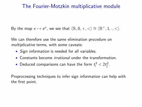
The Fourier-Motzkin multiplicative module
By the map x 7→ ex , we see that 〈R, 0,+, <〉 ∼= 〈R+, 1, ·, <〉.
We can therefore use the same elimination procedure onmultiplicative terms, with some caveats:
• Sign information is needed for all variables.
• Constants become irrational under the transformation.
• Deduced comparisons can have the form t3i < 2t2j .
Preprocessing techniques to infer sign information can help withthe first point.
The Fourier-Motzkin arithmetical modules
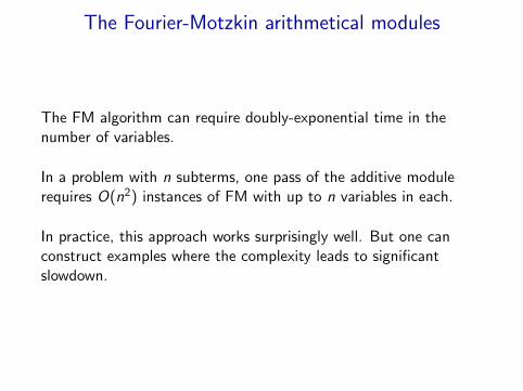
The FM algorithm can require doubly-exponential time in thenumber of variables.
In a problem with n subterms, one pass of the additive modulerequires O(n2) instances of FM with up to n variables in each.
In practice, this approach works surprisingly well. But one canconstruct examples where the complexity leads to significantslowdown.

The Geometric additive module
An alternative approach uses geometric insights.
A homogeneous linear equality in n variables defines an(n − 1)-dimensional hyperplane through the origin in Rn. Aninequality defines a half-space. A conjunction of inequalitiesdefines a polyhedron.
By projecting this polyhedron to the ti tj plane, one can find thestrongest implied comparisons between ti and tj .
x
z
y
x
y

Geometric arithmetical modules
We use the computational geometry packages cdd and lrs for theconversion from half-plane representation to vertex representation.
This approach scales better than the Fourier-Motzkin procedure.

Geometric multiplicative module
Translating this procedure to the multiplicative setting introducesa new problem:
5t22 t41 7→ log(5)︸ ︷︷ ︸
/∈Q
+2 log(t2) + 4 log(t1)
To avoid this, we introduce new variables
p2 = log(2), p3 = log(3), p5 = log(5), . . .
as necessary.

Axiom instantiation module
A highlight of our approach is its ability to prove theorems outsidethe theory of real closed fields.
An axiom instantiation module takes universally quantified axiomsabout function symbols and selectively instantiates them withsubterms from the problem.
Example:
Using axiom: (∀x)(0 < f (x) < 1)
Prove: f (a)3 + f (b)3 > f (a)3 · f (b)3

Axiom instantiation module
Unification must happen modulo equalities.
For example: we can unify f (v1 + v2):
Definitions Assignments Resultt1 = t2 + t3
t4 = 2t3 − t5
t6 = f (t1 + t4)
v1 7→ t2 − t5
v2 7→ 3t3f (v1 + v2) ≡ t6
We combine a standard unification algorithm with a Gaussianelimination procedure to find relevant substitutions.
Trigger terms can be specified by the user or picked by default.

Built-in functions
In addition to the arithmetic and axiom modules, Polya hasmodules that interpret specific functions.
• Exponentials and logarithms
• Minima and maxima
• Absolute values
• Various others

Exponential and logarithm module
The exponential module asserts axioms that say exp(x) is positiveand increasing.
It also adds identities of the forms
exp(c · t) = exp(t)c
exp(∑
ci ti
)=∏
exp (ci ti ) .
It adds similar axioms and identities for log(x), conditional onx > 0.

Minimum module
For any term t := min(c1t1, . . . , cntn), the minimum moduleasserts
t ≤ ci ti
(∀z)
(∧i
(z ≤ ci ti )→ z ≤ t
).
Since max(c1t1, . . . , cntn) = −min(−c1t1, . . . ,−cntn), it does notneed to be handled separately.

Absolute value module
The absolute value module asserts axioms
(∀x) (|x | ≥ 0 ∧ |x | ≥ x ∧ |x | ≥ −x)
(∀x) (x ≥ 0→ |x | = x)
(∀x) (x ≤ 0→ |x | = −x)
and looks for appropriate instantiations of the triangle inequality∣∣∣∑ ci ti
∣∣∣ ≤∑ |ci ti | .
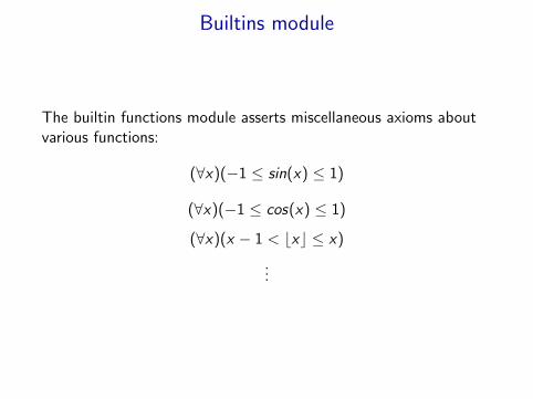
Builtins module
The builtin functions module asserts miscellaneous axioms aboutvarious functions:
(∀x)(−1 ≤ sin(x) ≤ 1)
(∀x)(−1 ≤ cos(x) ≤ 1)
(∀x)(x − 1 < bxc ≤ x)
...
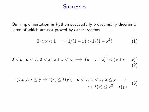
Successes
Our implementation in Python successfully proves many theorems,some of which are not proved by other systems.
0 < x < 1 =⇒ 1/(1− x) > 1/(1− x2) (1)
0 < u, u < v , 0 < z , z + 1 < w =⇒ (u + v + z)3 < (u + v +w)5
(2)
(∀x , y . x ≤ y → f (x) ≤ f (y)) , u < v , 1 < v , x ≤ y =⇒u + f (x) ≤ v2 + f (y)
(3)
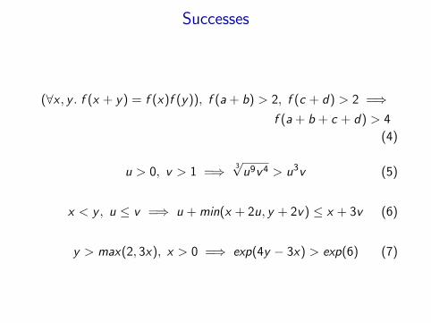
Successes
(∀x , y . f (x + y) = f (x)f (y)), f (a + b) > 2, f (c + d) > 2 =⇒f (a + b + c + d) > 4
(4)
u > 0, v > 1 =⇒ 3√u9v4 > u3v (5)
x < y , u ≤ v =⇒ u + min(x + 2u, y + 2v) ≤ x + 3v (6)
y > max(2, 3x), x > 0 =⇒ exp(4y − 3x) > exp(6) (7)
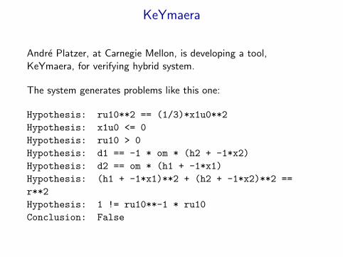
KeYmaera
Andre Platzer, at Carnegie Mellon, is developing a tool,KeYmaera, for verifying hybrid system.
The system generates problems like this one:
Hypothesis: ru10**2 == (1/3)*x1u0**2
Hypothesis: x1u0 <= 0
Hypothesis: ru10 > 0
Hypothesis: d1 == -1 * om * (h2 + -1*x2)
Hypothesis: d2 == om * (h1 + -1*x1)
Hypothesis: (h1 + -1*x1)**2 + (h2 + -1*x2)**2 ==
r**2
Hypothesis: 1 != ru10**-1 * ru10
Conclusion: False

KeYmaera
On a collection of 4442 problems generated automatically byKeYmaera, we solve over 95% with a 10-second timeout.
• 10 minutes using geometric packages
• 18 using Fourier-Motzkin

Limitations
Since our method is incomplete, it fails on a wide class of problemswhere other methods succeed.
x > 0, xyz < 0, xw > 0 =⇒ w > yz (8)
x2 + 2x + 1 ≥ 0 (9)
4 ≤ xi ≤ 6.3504 =⇒x1x4(−x1 + x2 + x3 − x4 + x5 + x6)
+ x2x5(x1 − x2 + x3 + x4 − x5 + x6)
+ x3x6(x1 + x2 − x3 + x4 + x5 +−x6)
− x2x3x4 − x1x3x5 − x1x2x6 − x4x5x6 > 0
(10)

Plans
Increase scope:
• Handle trigonometric functions, etc.
• Handle integer constraints.
• Handle second-order constructions: sums, products, integrals.
Draw on other methods:
• Make use of numerical information.
• Interact with numerical procedures (dReal, interval constraintpropagation).
• Make use of additional symbolic information (derivatives,gradients, convexity).
• Make use of algebraic procedures for real-closed fields.
• Make use of methods and systems for convex analysis.

Plans
Improve performance and search:
• Handle case splits and bactracking.
• Make the procedures incremental.
Make it proof-producing:
• Implement it in Lean.

References
For more information, see:
1. Avigad, Lewis, and Roux. A heuristic prover for realinequalities, Interactive Theorem Proving (Springer LNCS),2014.
2. Our revised, expanded version of the same paper.
3. Lewis’ 2014 MS thesis.
4. https://github.com/avigad/polya