A Guide to Singular Value Decomposition for

Collaborative FilteringChih-Chao Ma

Department of Computer Science, National Taiwan University, Taipei, Taiwan

Abstract

As the market of electronic commerce grows explosively, it is importantto provide customized suggestions for various consumers. Collaborativefiltering is an important technique which models and analyzes the prefer-ences of customers, and gives suitable recommendations. Singular ValueDecomposition (SVD) is one of the popular algorithms used for collabo-rative filtering. However, directly applying conventional SVD algorithmsto collaborative filtering may result in poor performance. In this report,we discuss problems that beginners may face and present effective SVDvariants for collaborative filtering.

1 Introduction

Collaborative filtering is a technique of predicting the preferences and interestsof users from the collections of taste information given by a large number ofusers. It has the basic assumption that people who agreed in the past will alsoagree in the future. Collaborative filtering can be used for a recommendationsystem that automatically suggests a user his/her preferred products.

1.1 Problem Definition

Suppose that a database collects the preferences of n users for m objects asnumerical scores. For example, a user can score a movie he or she has watchedby a rating of 1 − 5 stars. Usually, a user does not score all objects in thedatabase. Furthermore, some users may score many objects, but others onlyscore a few.

Let V ∈ Rn×m be the matrix of the collected scores in the database, andI ∈ {0, 1}n×m be its indicator such that Iij = 1 if object j is scored by user iand 0 if the score is missing. In most cases, V is sparse and unbalanced so thatthe numbers of scores for every user or object are unequal with a large variance.The existing scores in V work as the training data of collaborative filteringalgorithms, and the goal is to predict the missing scores in the database. LetA ∈ Rn×m be a sparse matrix including all or part of the missing votes as itsnonzero entries. A collaborative filtering algorithm aims to predict the valuesin A.

The performance of collaborative filtering can be measured by the errorbetween the prediction values and the ground-truth. A common and efficientmeasure is Root Mean Square Error (RMSE). Consider the prediction matrixP ∈ Rn×m and the ground-truth answer matrix A ∈ Rn×m. Let J ∈ {0, 1}n×m

be the indicator of A. The RMSE between the prediction P and the answer Ais defined as

RMSE(P,A) =

√∑ni=1

∑mj=1 Jij(Aij − Pij)2∑ni=1

∑mj=1 Jij

. (1)

1

Besides the function of error measurement, the formation and distributionof matrix A may also affect the evaluation of algorithms. For example, if thescores in A are randomly sampled from all existing scores in the database, auser who gives more scores in the database tends to have more scores in A.

A good example of test data generation is the Netflix Prize [Bennett andLanning, 2007], which is a grand contest for collaborative filtering on how peoplelike or dislike movies. The database used for the Netflix Prize contains over 100million scores for 480, 189 users and 17, 770 movies. The test data of the NetflixPrize, invisible to the competitors, are selected from the newest scores of eachuser. More precisely, they select a fixed number of most recent scores made byeach user, regardless of the total number of scores given by that user. Then,the collection of these newest scores is randomly divided into three sets, namedprobe, quiz, and test sets. The ground-truth scores of probe set are given to thecompetitors as well as other older scores in the database. The competitors arethen asked to predict the scores of quiz and test sets. Usually, the competitorsuse part of the training data to test their algorithms in an offline mode. Thatis, a validation dataset divided from the whole training data is needed.

These sets are generated so that the validation and test data have a simi-lar distribution. Since the test data are selected from the newest scores in thedatabase, this selection matches the goal of predicting future scores from pre-vious ones. The similarity between validation and test data ensures that theperformance of an algorithm is consistent in validation and testing. For eachuser, the number of unknown scores to be predicted is roughly the same. Hence,the error of predictions for users who gave only a few scores in the past tendsto be larger due to the lack of information. This situation is challenging tocollaborative filtering algorithms.

1.2 Related Work

Several conventional methods are available for collaborative filtering, and theyappear in the competition of the Netflix Prize. We briefly describe these meth-ods as well as their strengths and weaknesses. More details of some methodsare shown in later chapters.

The most intuitive way to predict the score of an object given by a user is toask other users who have scored the object. Instead of merely using the meanscore of that object among all users, we consider only those users similar tothe target user. This method is known as K-Nearest Neighbor, abbreviated asKNN. The KNN algorithm can be applied directly to the scores [Paterek, 2007],or to the residuals of another algorithm as a post-processing method [Bell et al.,2007a]. The key point of KNN methods is the definition of similarity. Usuallythe similarity is computed by the feature values of users and objects whichrepresent the characteristics of them in numerical values, but these features aredifficult to find.

Another type of method directly finds the feature values of each user andobject, and predicts the unknown scores by a prediction function using thosefeatures. Usually such algorithms involve a matrix factorization which con-structs a feature matrix for users and for objects, respectively. These kindsof algorithms includes Non-Negative Matrix Factorization and Singular ValueDecomposition, which have numerous variants and also play important roles inthe Progress Prize of the Netflix Prize in the year 2007 [Bell et al., 2007b].

2

These types of methods assumes that the score values depend on a predefinedprediction function.

Besides the widely-used algorithms described above, there are also othermethods which give good performance in the competition of the Netflix Prize.One of them uses a model called Restricted Boltzmann Machines [Salakhutdi-nov et al., 2007], which has proved to perform well in the Netflix Prize, eitherby itself or in a linear combination with other algorithms. Another approachis Regression, which predicts the unknown scores by taking the scores in thetraining data as observations. On the other hand, if one wants to combine theresults of several algorithms for better accuracy, regression is also useful to findthe weights of linear combination.

1.3 Summary

In this report, we focus on Singular Value Decomposition, which is the mostpopular algorithm for the Netflix Prize. Section 2 shows details of SVD al-gorithms, including the conventional way used for information retrieval andvariants which are more suitable for collaborative filtering. We find that thechoice of optimization methods is important for SVD algorithms to give goodperformance. In Section 3 we give the experimental results of algorithms. Theconclusions are given in Section 4.

2 Singular Value Decomposition

Singular Value Decomposition, abbreviated as SVD, is one of the factorizationalgorithms for collaborative filtering [Zhang et al., 2005]. This type of algorithmfinds the features of users and objects, and makes predictions based on thesefactors. Some factorization algorithms have additional restrictions on each singlefeature value, or between the feature vectors of multiple users, but SingularValue Decomposition does not impose restrictions and is easier to implement.

2.1 Formulation

Suppose V ∈ Rn×m is the score matrix of m objects and n users, and I ∈{0, 1}n×m is its indicator. The SVD algorithm finds two matrices U ∈ Rf×n

and M ∈ Rf×m as the feature matrix of users and objects. That is, each user orobject has an f -dimension feature vector and f is called the dimension of SVD.A prediction function p is used to predict the values in V . The value of a scoreVij is estimated by p(Ui,Mj), where Ui and Mj represent the feature vector ofuser i and object j, respectively. Once U and M are found, the missing scoresin V can be predicted by the prediction function.

The optimization of U and M is performed by minimizing the sum of squarederrors between the existing scores and their prediction values:

E =12

n∑i=1

m∑j=1

Iij(Vij − p(Ui,Mj))2 +ku

2

n∑i=1

‖Ui‖2 +km

2

m∑j=1

‖Mj‖2, (2)

where ku and km are regularization coefficients to prevent overfitting.The most common prediction function is the dot product of feature vectors.

That is, p(Ui,Mj) = UiTMj . The optimization of U and M thus becomes a

3

matrix factorization problem where V ≈ UTM . But in most applications, scoresin V are confined to be in an intervel [a, b], where a and b are the minimal andmaximal score values defined in the domain of data. For example, if the usersrate the objects as 1− 5 stars, then the scores are bounded in the interval [1, 5].One way is to clip the values of dot products. For example, we can bound thevalues of Ui

TMj in the interval [0, b− a] and the prediction function becomes aplus the bounded dot product. Hence, the prediction function is:

p(Ui,Mj) =

a if Ui

TMj < 0,a+ Ui

TMj if 0 ≤ UiTMj ≤ b− a,

b if UiTMj > b− a.

(3)

When using the prediction function (3), the objective function and its neg-ative gradients have the following forms:

E =12

n∑i=1

m∑j=1

Iij(Vij − p(Ui,Mj))2 (4)

+ku

2

n∑i=1

‖Ui‖2 +km

2

m∑j=1

‖Mj‖2,

− ∂E∂Ui

=m∑

j=1

Iij ((Vij − p(Ui,Mj))Mj)− kuUi, i = 1, ..., n, (5)

− ∂E

∂Mj=

n∑i=1

Iij ((Vij − p(Ui,Mj))Ui)− kmMj , j = 1, ...,m. (6)

One can than perform the optimization of U and M by gradient descent:

Algorithm 1 (Batch learning of Singular Value Decomposition)Select a learning rate µ, and regularization coefficients ku, km.

1. Set the starting values of matrices U,M .

2. Repeat

(a) Compute gradients ∇U and ∇M by (5) and (6).(b) Set U ← U − µ∇U , M ←M − µ∇M .

until the validation RMSE starts to increase.

The tuneable parameters are the learning rate µ, and the regularizationcoefficients ku and km for user and object features, respectively. The learningrate affects the learning time, and too large a value may lead to divergence. Ingeneral, a smaller learning rate gives better performance, but the learning timeis also longer.

Another setting that affects the performance is the starting point of featurevalues. One way is to use random values in a specific range, but unstableperformances may occur if these values are too random. In Algorithm 1, thestarting point can be the average of all existing scores V̄ :

Uij ,Mij =

√V̄ − af

+ n(r) for each i, j, (7)

4

where a is the lower bound of scores, f is the dimension of SVD algorithms,and n(r) is a random noise with uniform distribution in [−r, r]. According tothe prediction function (3), it is likely to predict all values to the global averageV̄ with some noises at the start of the algorithm. Without the random noise in(7), the features of a user or an object will be the same as they always have thesame gradients during optimization. A small value of r is usually enough.

Batch learning is the standard method for SVD. However, it is not good fora large-scale but sparse training matrix V , which is common for collaborativefiltering. The values of the gradients have a large variance under such a situation,and a small learning rate is required to prevent divergence. In Section 2.2, weshow some more suitable variants for collaborative filtering.

2.2 Variants of SVD

We have mentioned that batch learning may not perform well. Instead, one canuse incremental learning, which modifies only some feature values in U and Mafter scanning part of the training data. For example, if one user i is consideredat a time, the variables related to this user are:

(1) Ui: the feature vector of user i,(2) each Mj with Iij = 1: the feature vectors of objects scored by user i.

If one considers only terms related to user i, the objective function becomes:

Ei =12

m∑j=1

Iij(Vij − p(Ui,Mj))2 +ku

2‖Ui‖2 +

km

2

m∑j=1

Iij

(‖Mj‖2

), (8)

with the negative gradients

− ∂Ei

∂Ui=

m∑j=1

Iij ((Vij − p(Ui,Mj))Mj)− kuUi, (9)

− ∂Ei

∂Mj= Iij ((Vij − p(Ui,Mj))Ui)− kmIij (Mj)

= Iij [(Vij − p(Ui,Mj))Ui − kmMj ] , j = 1, ...,m. (10)

Note that if Iij = 0, then the gradients of Mj is 0. Hence the variables of anobject not scored by user i are not updated.

This incremental learning approach is different from batch learning, as thesum of Ei over all users does not lead to the objective function E given in (4):

n∑i=1

Ei =12

n∑i=1

m∑j=1

Iij(Vij − p(Ui,Mj))2 (11)

+ku

2

n∑i=1

‖Ui‖2 +km

2

m∑j=1

n∑i=1

Iij

(‖Mj‖2

).

Each object feature vectorMj has an additional regularization coefficient∑n

i=1 Iij ,which is equal to the number of existing scores for object j. Therefore, an ob-ject with more scores has a larger regularization coefficient in this incrementallearning approach.

5

An extreme case of incremental learning is to update the features after look-ing at each single score. That is, we consider the following objective functionand negative gradients for each Vij which is not missing:

Eij =12

(Vij − p(Ui,Mj))2 +ku

2‖Ui‖2 +

km

2‖Mj‖2, (12)

−∂Eij

∂Ui= (Vij − p(Ui,Mj))Mj − kuUi, (13)

−∂Eij

∂Mj= (Vij − p(Ui,Mj))Ui − kmMj . (14)

We denote this type of learning as complete incremental learning, and the one in(8), which considers multiple scores at a time as incomplete incremental learning.

The summation of Eij over all existing votes is

n∑i=1

m∑j=1

Eij =12

n∑i=1

m∑j=1

Iij(Vij − p(Ui,Mj))2 (15)

+ku

2

n∑i=1

m∑j=1

Iij

(‖Ui‖2

)+km

2

m∑j=1

n∑i=1

Iij

(‖Mj‖2

).

In this case, each user and object has a regularization coefficient which is pro-portional to the number of existing scores related to that user or object.

The following algorithms describe the optimization of U and M with incre-mental learning. Algorithm 2 performs incomplete incremental learning, andAlgorithm 3 does complete incremental learning, which updates the feature val-ues after examining each single score. The starting points of U and M in thesealgorithms can also be (7).

Algorithm 2 (Incomplete incremental learning of Singular Value Decomposition)Select a learning rate µ, and regularization coefficients ku, km.

1. Set the starting values of matrices U,M .

2. Repeat

(a) For i = 1 to n

i. Compute gradients ∇Uiby (9).

ii. Compute gradients ∇Mjby (10) for j = 1 to m.

iii. Set Ui ← Ui − µ∇Ui.

iv. Set Mj ←Mj − µ∇Mj for j = 1 to m.

until the validation RMSE starts to increase.

Algorithm 3 (Complete incremental learning of Singular Value Decomposition)Select a learning rate µ, and regularization coefficients ku, km.

1. Set the starting values of matrices U,M .

2. Repeat

(a) For each existing score Vij in training data

6

i. Compute gradients ∇Uiand ∇Mj

by (13) and (14).ii. Set Ui ← Ui − µ∇Ui

, Mj ←Mj − µ∇Mj.

until the validation RMSE starts to increase.

Algorithms 2 and 3 cause different optimization results and performance, asthe sums of objective functions (11) and (15) are different when regularizationis used. If we modify the objective function (8) to

Ei =12

m∑j=1

Iij(Vij − p(Ui,Mj))2 (16)

+ku

2

m∑j=1

Iij

(‖Ui‖2

)+km

2

m∑j=1

Iij

(‖Mj‖2

),

then the sums of objective functions will be the same. In Section 3, we will usethis approach for the comparison between incomplete and complete incrementallearning in the experiments.

Instead of using incremental learning, we can also increase the learning speedof batch learning by adding a momentum λ in the gradient descent procedure.That is, Algorithm 1 is modified to the following Algorithm:

Algorithm 4 (Batch learning of SVD with Momentum)Select a learning rate µ, and regularization coefficients ku, km.

1. Set the starting values of matrices U,M .

2. Set the movement of matrices ∆U ← 0f×n,∆M ← 0f×m.

3. Repeat

(a) Set ∆U ← λ∆U,∆M ← λ∆M .

(b) Compute gradients ∇U and ∇M by (5) and (6).

(c) Set ∆U ← ∆U − µ∇U ,∆M ← ∆M − µ∇M

(d) Set U ← U + ∆U , M ←M + ∆M .

until the validation RMSE starts to increase.

Batch learning usually suffers from divergence when using the same learningrate as incremental learning, but a small value of learning rate also makes thealgorithm infeasible in time. The momentum term can accumulate the move-ments of variables, making the optimization faster under a small learning rate.In small-scale data sets, batch learning can outperform incremental learning byadding the momentum term. However, batch learning cannot give reasonableperformances in large-scale data sets even with the momentum.

One can perform line search to find a better learning rate for gradient de-scent. This approach requires fewer iterations, but its computation time islonger due to the overhead of line search.

7

2.3 Further Improvements

With proper optimization settings, the SVD algorithm is able to give a goodperformance. However, some variants have the potential to make more accuratepredictions. A simple one is to add a per-user bias α ∈ Rn×1 and a per-objectbias β ∈ Rm×1 on the prediction function [Paterek, 2007]:

p(Ui,Mj , αi, βj) = a+ UiTMj + αi + βj , (17)

where αi is the bias of user i and βj is the bias of object j.The biases are updated like the feature values. For the “complete incre-

mental learning,” using a single score Vij at a time gives the following negativegradients of bias αi and βj :

Eij =12

(Vij − p(Ui,Mj , αi, βj))2 (18)

+ku

2‖Ui‖2 +

km

2‖Mj‖2 +

kb

2(α2

i + β2j ),

−∂Eij

∂αi= (Vij − p(Ui,Mj , αi, βj))− kbαi, (19)

−∂Eij

∂βj= (Vij − p(Ui,Mj , αi, βj))− kbβj , (20)

where kb, the regularization coefficient of biases, is similar to km and ku. Ofcourse, the learning rate of the biases can be different from each other.

Another variant of SVD algorithms, called constrained SVD, adds additionalconstraints to each user feature vector Ui [Salakhutdinov and Mnih, 2008]. Inthis algorithm, the user feature matrix U ∈ Rf×n is replaced by a matrix Y ∈Rf×n of the same size, and an object constraint matrix W ∈ Rf×m shifts thevalues of user features:

Ui = Yi +∑m

k=1 IikWk∑mk=1 Iik

, (21)

where Wk is the k-th column of the matrix W . In other words, the feature vectorUi is the user-dependent feature vector Yi plus an offset

Pmk=1 IikWkPm

k=1 Iik, which is

the mean of object constraint feature vectors on the objects scored by user i.Each Wk contributes to a user feature Ui if user i scores object k.

Under this setting, the prediction function becomes:

p(Ui,Mj) = a+(Yi +

∑mk=1 IikWk∑m

k=1 Iik

)T

Mj , (22)

and the values of Y and W can also be updated by gradient descent with theuse of regularization coefficients ky and kw. However, the optimization hasa high time complexity for complete incremental learning. We give furtherdiscussion and propose a feasible solution, called compound SVD, in [Ma, 2008].A compound SVD algorithm which combines the biases and constraints is used,and it gives a significantly better performance than the SVD algorithm withcomplete incremental learning.

8

3 Experiments

We use the Movielens data set [Miller et al., 2003], the Netflix data set [Bennettand Lanning, 2007], and three smaller data sets sampled by the Netflix data setfor evaluation. Each data set is divided into two disjointed training and testsets. The performances are measured by test RMSE (1), which is presentedalong with training time.

3.1 Data Sets

The Movielens data set is provided by GroupLens [Konstan et al., 1997], aresearch group which collects and supplies several collaborative filtering datain different domains. The data set contains 1, 000, 209 scores for 6, 040 usersand 3, 706 movies. Each user gives at least 20 scores. Since the data set doesnot come with a training and test split, we randomly select three scores fromeach user as test data. Hence the ratio of training and test sets is similar to theNetflix data set.

The other data set is given by the Netflix Prize as mentioned in Section 1.There are 100, 480, 507 scores for 480, 189 users and 17, 770 movies. Each userhas at least 20 scores in the beginning, but the competition organizers inten-tionally perturb the data set so some users may have less than 20 scores. Thetest data used for experiments are exactly the probe set provided by the NetflixPrize, which includes 1, 408, 395 scores. The training data are the remaining99, 072, 112 scores.

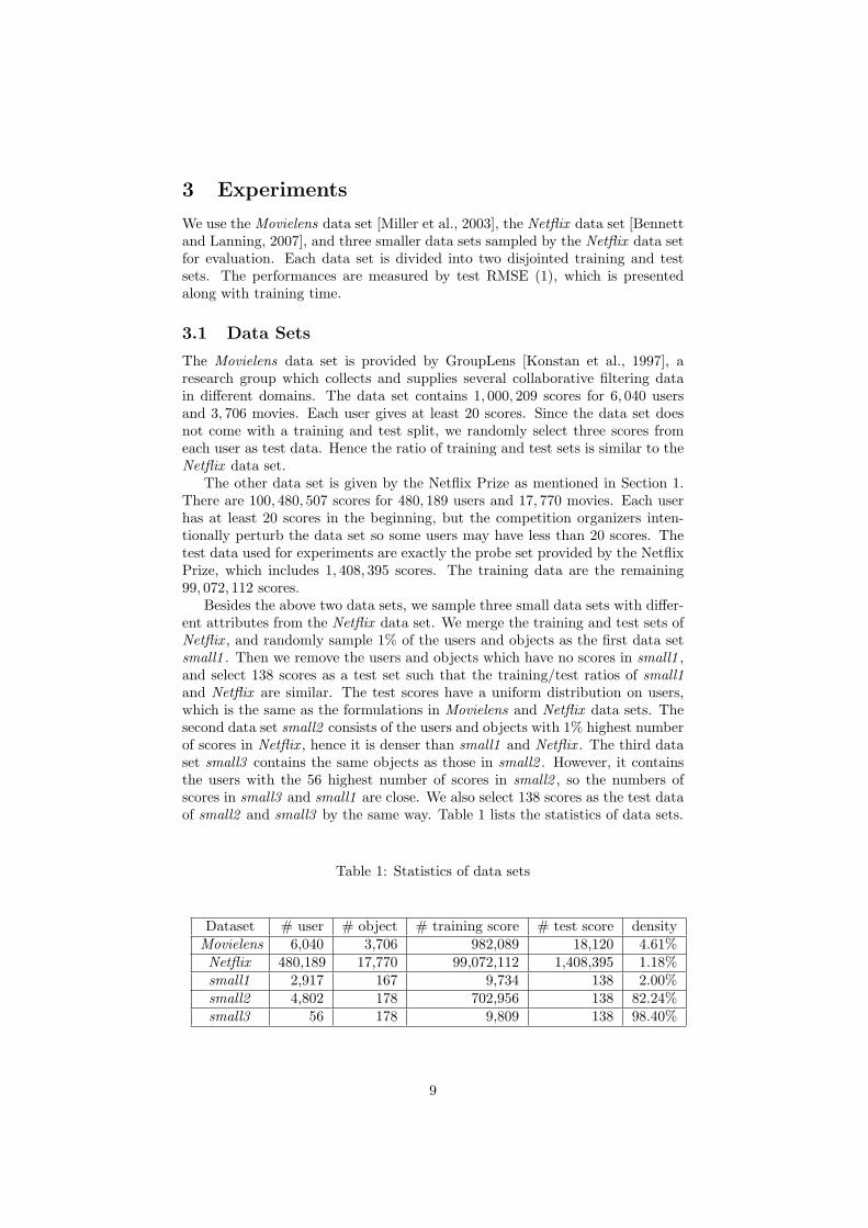
Besides the above two data sets, we sample three small data sets with differ-ent attributes from the Netflix data set. We merge the training and test sets ofNetflix , and randomly sample 1% of the users and objects as the first data setsmall1 . Then we remove the users and objects which have no scores in small1 ,and select 138 scores as a test set such that the training/test ratios of small1and Netflix are similar. The test scores have a uniform distribution on users,which is the same as the formulations in Movielens and Netflix data sets. Thesecond data set small2 consists of the users and objects with 1% highest numberof scores in Netflix , hence it is denser than small1 and Netflix . The third dataset small3 contains the same objects as those in small2 . However, it containsthe users with the 56 highest number of scores in small2 , so the numbers ofscores in small3 and small1 are close. We also select 138 scores as the test dataof small2 and small3 by the same way. Table 1 lists the statistics of data sets.

Table 1: Statistics of data sets

Dataset # user # object # training score # test score densityMovielens 6,040 3,706 982,089 18,120 4.61%

Netflix 480,189 17,770 99,072,112 1,408,395 1.18%small1 2,917 167 9,734 138 2.00%small2 4,802 178 702,956 138 82.24%small3 56 178 9,809 138 98.40%

9

3.2 Experimental Results

We implement the SVD algorithms in C, since they are the most time-consumingin computation. We use MATLAB for data preprocessing and postprocessing asit is convenient for matrix manipulation. For different SVD algorithms, the testRMSEs are plotted against the training time. Algorithms used for comparisonare listed below:AVGB: A simple baseline predictor that predicts the score Pij for user i andobject j as µj + bi, where µj is the mean score of object j in training data, andbi is the average bias of user i computed as:

bi =

∑mj=1 Iij(Vij − µj)∑m

j=1 Iij. (23)

SVD: Algorithm 3, which uses incremental learning with regularization terms.SVDNR: It is the same as algorithm SVD but has the regularization coeffi-cients set to 0. This algorithm works as another baseline.SVDUSER: The SVD algorithm which has the same gradients as SVD, butuses incomplete incremental learning which updates the feature value after scan-ning all scores of a user instead of each single score.SVDBATCH: Algorithm 4, which use batch learning with a learning momen-tum 0.9.CSVD: A compound SVD algorithm which incorporates per-user and per-object biases and the constraints on feature vectors. Implementation detailsare described in [Ma, 2008].

First, we give a comparison between batch learning and incremental learning.We apply SVDNR and SVDBATCH on the data sets, where the regulariza-tion coefficients of SVDBATCH are set to 0. The test RMSEs with respectto training time for the four data sets small1 , small2 , small3 , and Movielensare shown in Figure 1. The learning rate in SVDNR is 0.005 for each data set.For the algorithm SVDBATCH, the learning rates are 0.0005, 0.0003, 0.001and 0.0002 for small1 , small2 , small3 , and Movielens, respectively. These val-ues give the lowest RMSEs in the shortest time without making the algorithmdiverge.

Batch learning with a high learning momentum has similar performances toincremental learning in small data sets, but the decrease of RMSE is usuallyunstable. Batch learning is considered inefficient in medium or large data setslike Movielens or Netflix . In figure 1, SVDBATCH needs more training timeto give the same performance for Movielens data set. Moreover, SVDBATCHrequires over 10, 000 seconds to get the lowest RMSE for Netflix data set, whileSVDNR takes about 300 seconds to reach a similar RMSE.

Then, we show the performances of SVDNR, SVD, SVDUSER, andCSVD for two larger data sets Movielens and Netflix . For each data set, thematrices M,U in SVDNR, SVD and SVDUSER as well as M,Y in CSVDare initialized by (7). The values of the constraint matrix W and biases α, β inCSVD are all initialized as 0. As parameters, the learning rate µv in SVDNRand SVD is 0.003 for the Movielens data set and 0.001 for the Netflix dataset, but SVDUSER uses various learning rates for comparison. The regular-ization coefficients ku, km are 0 in SVDNR, while SVD and SVDUSER useregularization coefficients leading to the best performances, which are both 0.05

10

Figure 1: Plots of RMSE on batch and incremental learning

Table 2: Best RMSE achieved by each algorithm

Dataset AVGB SVDNR SVD CSVDMovielens 0.9313 0.8796 0.8713 0.8706

Netflix 0.9879 0.9280 0.9229 0.9178

for Movielens and both 0.005 for Netflix . The algorithm CSVD has more pa-rameters than other algorithms, but its learning rates µv and µw are the sameas µv in SVDNR and SVD, and its first two regularization coefficients ky, km

are also equal to ku, km in SVD. The other regularization coefficient kw forthe constraint matrix W is 0.02 for Movielens and 0.001 for Netflix . For thebiases in CSVD, the learning rate and regularization coefficient (µb, kb) are(0.0005, 0.05) for Movielens and (0.0002, 0.005) for Netflix . All these SVD-likealgorithms have the dimension f = 10.

Table 2 shows the best RMSEs achieved by algorithms AVGB, SVDNR,SVD, and CSVD. That is, the lowest test RMSEs given by those algorithmsbefore overfitting. We show the RMSEs versus training time in Figure 2, includ-ing algorithm SVDUSER with different learning rates. SVDNR suffers fromoverfitting quickly as it does not have a regularization term, while SVD gives abetter performance with the same learning rate. CSVD is the best algorithmfor both data sets, but it does not outperform SVD too much in Movielens

11

Figure 2: Plots of RMSE on the SVD-like algorithms

as its assumption on user features are not effective in a denser data set. Thebehavior of SVDUSER shows that incomplete incremental learning is a badchoice. It can still lead to similar performances if the same gradients are used,but a smaller learning rate and more training time are needed. If the learningrate is not small enough, the decrease of RMSE is even unstable, so it is hardto decide the stopping condition of an algorithm. Batch learning also has thesame problem as incremental learning does. In our experiments, batch learn-ing requires an extremely small learning rate to reach the same performanceas complete incremental learning, and it even takes several days to completethe optimization for Netflix . In conclusion, complete incremental learning isbetter in the optimization of SVD algorithms for collaborative filtering, and thecompound SVD algorithm can further boost the performances of conventionalSVD algorithms for a sparse data set like Netflix .

At last, we show the effect of increasing the dimension of SVD. We use thealgorithm SVD with dimension f = 20, 30, 50 and 100. The regularizationcoefficients ku and km are both 0.015, which is suitable for each number ofdimension in the experiments. The results are shown in Figure 3. The increase ofdimension does raise the performance, but the training time is also proportionalto the number of dimension.

In the Netflix Prize contest, the dimensions of SVD-like algorithms are usu-ally set to a large value for lower RMSE. On the other hand, the training dataof Netflix in our experiments contain only 99, 072, 112 scores as we need a vali-dation set, but it is better to run the algorithm with the full training data with100, 480, 507 scores, using the best parameters found by the training/validation

12

Figure 3: Plots of RMSE on the SVD algorithms with different dimensions

split. This approach decreases the test RMSE by about 0.005 − 0.01. For theNetflix Prize competition, we use the algorithm CSVD with dimension f = 256,followed by a post processing method described in [Ma, 2008]. The RMSE ofour best result is 0.8868.

4 Conclusions

A careful implementation of Singular Value Decomposition is effective for col-laborative filtering. Our experiments show that, in general, batch learning orincomplete incremental learning requires a smaller learning rate, and has anunstable performance than complete incremental learning. We find that in-cremental learning, especially completely incremental learning which updatesvalues after looking at a single training score, is the best choice for collaborativefiltering with millions of training instances.

References

R. Bell, Y. Koren, and C. Volinsky. Modeling relationships at multiple scales toimprove accuracy of large recommender systems. In KDD ’07: Proceedingsof the 13th ACM SIGKDD international conference on Knowledge discoveryand data mining, pages 95–104, New York, NY, USA, 2007a. ACM. ISBN978-1-59593-609-7. doi: http://doi.acm.org/10.1145/1281192.1281206.

R. Bell, Y. Koren, and C. Volinsky. The BellKor solution to the NetflixPrize. 2007b. URL http://www.research.att.com/~volinsky/netflix/ProgressPrize2007BellKorSolution.pdf.

J. Bennett and S. Lanning. The Netflix Prize. Proceedings of KDD Cup andWorkshop, 2007.

13

J. A. Konstan, B. N. Miller, D. Maltz, J. L. Herlocker, L. R. Gordon, andJ. Riedl. GroupLens: applying collaborative filtering to Usenet news. Com-munications of the ACM, 40(3):77–87, 1997. ISSN 0001-0782. doi: http://doi.acm.org/10.1145/245108.245126.

C.-C. Ma. Large-scale collaborative filtering algorithms. Master’s thesis,National Taiwan University, 2008. URL http://www.csie.ntu.edu.tw/

~r95007/thesis/svdnetflix/thesis.pdf.

B. N. Miller, I. Albert, S. K. Lam, J. A. Konstan, and J. Riedl. Movielensunplugged: experiences with an occasionally connected recommender system.In IUI ’03: Proceedings of the 8th international conference on Intelligent userinterfaces, pages 263–266, New York, NY, USA, 2003. ACM. ISBN 1-58113-586-6. doi: http://doi.acm.org/10.1145/604045.604094.

A. Paterek. Improving regularized Singular Value Decomposition for collabora-tive filtering. Proceedings of KDD Cup and Workshop, 2007.

R. Salakhutdinov and A. Mnih. Probabilistic Matrix Factorization. In J. Platt,D. Koller, Y. Singer, and S. Roweis, editors, Advances in Neural InformationProcessing Systems 20, pages 1257–1264. MIT Press, Cambridge, MA, 2008.

R. Salakhutdinov, A. Mnih, and G. Hinton. Restricted Boltzmann Machines forcollaborative filtering. In Proceedings of the 24th international conference onMachine learning, pages 791–798, New York, NY, USA, 2007. ACM. ISBN978-1-59593-793-3. doi: http://doi.acm.org/10.1145/1273496.1273596.

S. Zhang, W. Wang, J. Ford, F. Makedon, and J. Pearlman. Using SingularValue Decomposition approximation for collaborative filtering. Seventh IEEEInternational Conference on E-Commerce Technology, 2005. CEC 2005.,pages 257–264, July 2005. ISSN 1530-1354. doi: 10.1109/ICECT.2005.102.

14