1

A Guide to Design MIMO Controllers for Architectures

Raghavendra Pradyumna Pothukuchi and Josep TorrellasUniversity of Illinois at Urbana-Champaign

http://iacoma.cs.uiuc.eduApril 2016

F

1 INTRODUCTION

Adapting hardware components to achieve multiple design objectives is a challenging task because of many reasons.First, there are multiple objectives that could present opposing tradeoffs. These objectives or outputs could be ofvarying importance – some are more important than others. There are multiple reconfigurable parameters or inputswith different degrees of influence on the objectives, and different overheads of change. All these considerationsare further complicated by the many ways in which applications use and respond to hardware changes. Owing tothese challenges, there has not been a clear methodology that can help architects to design adaptation controllersfor the general case. As a result, most adaptation controllers either use multiple decoupled controllers that ignoreinteraction across objectives and hardware parameters, or resort to ad hoc solutions based on the specific natureof the adaptation scenario. Obviously, this approach can not be extended to the general case nor there is assurancethat the piece-meal controllers work well with each other. Therefore, these controllers that are designed and tunedby focusing on a limited set of scenarios or hardware interactions can often result in major bugs or sub-optimalactions when they encounter a situation different from what they are trained on.

An alternative approach is to use control theory that combines the designer intuition with rigorous methodologiesto generate reliable and optimal adaptation controllers. Specifically, we need what is called as Multiple InputMultiple Output (MIMO) control. In this method, the designer specifies the information he/she has about thedesign such as the priorities of the output or the overheads of changing inputs. The underlying algorithms generatea controller that meets multiple objectives by actuating on multiple inputs simultaneously. The interactions betweenthe inputs and outputs are represented in a structured manner and the final controller is able to take better decisions,being aware of all these interactions. Unfortunately, there has not been prior work that interfaces MIMO controltheory with computer architecture. In [1], we address this issue by describing MIMO controller design and thearchitectural insights into this process. This would help the architect to use this powerful tool to create efficientadaptation controllers. The purpose of [1] was to shed light on the MIMO controller design process from thearchitecture side. It does not describe in detail the specific design methods and analysis one has to perform todesign a MIMO controller for architecture. This manual addresses this gap.

In this manual, we describe how the methods and analysis from MIMO Control Theory, System Identification andRobust Control Design are applied to design architectural controllers. We focus on a specific type of MIMO controllercalled the Linear Quadratic Gaussian (LQG) controller for architecture adaptation, similar to [1]. We present thedifferent choices that the designer has in this process and some recommendations based on our experience. We alsolist the commands from MATLAB and Simulink that we use to design the example MIMO controller in [1]. Wehope that by the end of the manual, the reader would be aware of the details of all the steps required to design aMIMO controller for architecture and can successfully design such a controller for the system of his/her choice.

2 BACKGROUND

In this section, we first present a short summary of the LQG controller, its working and design process from [1].Then, we introduce the tools needed for LQG controller design and some background material that helps in therobustness analysis of the LQG controller we design.

2.1 LQG ControllerAn LQG (Linear Quadratic Gaussian) controller is a type of MIMO controller to minimize tracking errors in theoutputs. The controller first infers the state of the system being controlled from the system outputs and then producessystem inputs to keep the system outputs close to their desired values. Moreover, the inputs are generated such thata designer specified cost function is minimized. This cost function is the sum of two costs that respectively capturethe penalties of not meeting the output targets and the penalties of rapidly changing the inputs. These costs haveweights that the designer can specify. This cost function with the weights is shown in Equation 1.

2

J = (∆yT ×Q×∆y) + (∆uT ×R×∆u) (1)

In Equation 1, ∆y denotes the difference between the values of outputs and the desired reference values forthese outputs. ∆u is the difference between the current input and the proposed new value of the input. Q is adiagonal matrix with positive entries that indicate the relative importance of meeting different output targets. Ris also a diagonal matrix that specifies the relative preference for changing inputs. For example, when we haveinputs with different levels of quantization, we would want to apply small changes to the input with many levels,taking advantage of the fine grained quantization. In another scenario, we might have an input that has a largeoverhead to change compared to another, such as power gating a core vs resizing the reorder buffer. We wouldwant to prefer changing the low overhead input more often than the higher overhead input. Through the Q andR matrices in the cost function, the architect can convey the design goals to the LQG methodology.

LQG control also allows a system to be characterized as the combination of a deterministic part and an unknownpart that follows a Gaussian distribution. This stochastic component accounts for unpredictable effects, programbehavior, sensor noise and other effects on the outputs that are not caused by the inputs. This makes the controllermore reliable and useful in a wide variety of scenarios.

Since we rely on a model for LQG controller design, we need to check that the controller we design is robustto modeling errors. Complicated systems such as a processor cannot always be accurately described using modelsand model errors are very likely to occur. The controller we design should be able to work correctly and providestability guarantees even when the true system deviates from this model. This is achieved through Robust Stability.It is a type of analysis that lets the designer specify a model confidence level or guardband for the model accuracy.Then, it checks that the designed controller is robustly stable for all conditions that do not consistently deviate thesystem from the model by more than the specified guardband.

2.2 Working of the LQG ControllerThe LQG controller generates the system inputs, based on the state of the system and the difference between theoutputs of the system and their target values. However, as the system’s true state is not known, the controllerbegins with a state estimate and generates the system inputs based on this estimate. The controller refines theestimate and learns the true state by comparing the output predicted using the state estimate and the true output.Both estimation and system input generation happen simultaneously and their accuracy increases with time. Thedesign of the LQG controller guarantees that the estimated state converges to the unknown true state soon and,therefore, the appropriate input values are generated to stabilize the system outputs at their target values quickly.

Figure 1 describes these two parts of the LQG controller. The part of the controller that estimates the state of thesystem is called the estimator. It takes in the system inputs (u(T )) and outputs (y(T )) to produce the state estimate(x(T )) and output estimate y(T ), based on the state estimate. The state estimate is refined by comparing y(T ) withthe true output y(T ). At the same time, the optimal tracker generates system inputs u(T ) using the estimatedstate x(T ) and ∆y(T ), the deviation of y(T ) from the references, y◦(T ). (In reality, the estimator in Figure 1 worksusing ∆y(T ), instead of y(T ).) The LQG design step produces a single set of matrices that perform both functionssimultaneously. This is the LQG controller shown using the box with dashed lines. Observe that there are two typesof feedback in this structure. The optimal tracker feedback is trying to change the inputs by observing the trackingerror of the outputs. The estimator feedback is making the control action precise by observing the system outputsand refining the controller’s view of the system state. Both feedback mechanisms allow the controller to adapt toa wide variety of workloads and reduce tracking errors according to the specified cost function.

2.3 Designing the LQG ControllerThe general process for the LQG controller design as is shown in Figure 2. In [1], we limited our discussion tothe architectural insights into the different design steps of MIMO controller design – i.e., the hexagonal boxes inFigure 2. We cover all the steps in this manual and show how to practically design an LQG controller using theinsights from [1].

This manual is organized as follows:Section 3: Defining the System – Choosing inputs, outputs, their weights and modeling strategy.Section 4: System Identification setup – Design experiments to obtain data that can be used for model devel-

opment.Section 5: System Identification – Use MATLAB to identify a good model and its uncertainty from experimental

data.Section 6: LQG Design and Tuning – Use MATLAB to design and tune the LQG controller comprising the

estimator and optimal tracker.

3

Optimal

TrackerSystem+__

Target

error

Estimator

+

__

y(T) u(T) y(T)

x(T)y(T)

LQG

Controller

oy (T)

Fig. 1: Internal working of the LQG controller showing the estimator and optimal tracker

Begin

Select Outputs

+ Targets

Select Inputs

Decide

importance of

Outputs

Decide

overhead of

Inputs

Decide

modeling

strategy

Generate

experimental

Data

MATLAB

A, B, C, D and

Unpredictability

R

Q

MATLAB

Validate model

& Estimate error

Design

controller

Meets

targets?

Decide

uncertainty

Robust? DeployYes Yes

No No

Fig. 2: Flowchart of the process of building a MIMO controller

Section 7: Robust Stability Analysis – Use MATLAB to analyze the robustness of the LQG controller designedin the previous step.

In this manual, MATLAB commands are specified in bold typewriter font, variable names are shown intypewriter font, and options or menu names are shown in italicized font.

The Appendix describes the design of heuristic algorithms that we use to compare with the MIMO controllerin [1]. We also present some qualitative differences of heuristic control over MIMO control in the Appendix.

2.4 Design ToolsThere are two main tools, MATLAB and Simulink that we need to design the LQG controller, apart from theplatform to run experiments and collect results (the simulator ESESC in our case).

MATLAB is a numerical computing framework and programming language. You can enter commands in theMATLAB commandline or write scripts. Iterative tasks such as controller tuning are usually scripted. The helpcommand followed by a command gives detailed description of the command, often with examples.

Simulink is the GUI (Graphical User Interface) environment attached to MATLAB. It is a graphical environmentfor modeling and simulating systems as block diagrams. It can be launched by the MATLAB command simulinkor from the MATLAB Toolstrip.

Both MATLAB and Simulink are easy to use and have extensive documentation. There are many online resourcesfor these tools. A very good starting guide for MATLAB is [2]. An excellent introduction to Simulink is given in [3].Other introductory resources for MATLAB are [4], [5]. Some tutorials on MATLAB, Simulink and their use inControl Systems are available in [6]. More information on MATLAB/Simulink commands can be obtained fromonline documentation by MathWorks Inc., the developers of these tools. The command help followed by anotherMATLAB command provides a good description of the command, often with examples.

It is strongly advised to consult resources such as [2] and [3] while or before reading this manual. It will greatlyreduce the effort needed to interact with these tools.

Here we give a short summary on how to use Simulink:

4

Simulink contains many libraries that have different types of models with configurable parameters. For example,the Control System Toolbox has the LTI System block that is used for simulating a model or controller design. Wecan add custom models and libraries. To design a model or simulation, create a new model, drag and drop therequired models (or blocks) from the existing libraries. The blocks are connected by drawing wires between them.Wires can be placed between the blocks by clicking and dragging the mouse. Set the properties for each of theblocks. The properties window for any Simulink block can be viewed through a double-click or a single right-click.We can specify the duration of the simulation and select Run to carry out the simulation.

In the Library Browser, different types of waveform sources are in the Sources set of the Simulink library. Thesignals can be viewed using Scopes in the Sinks set of the same library. When you add a scope, uncheck the limitedhistory feature in the History menu of the scope parameters. You can enable the legend by selecting the checkboxin the General menu. Each wire/connection can be given a name by double-clicking it like other blocks. This namewill appear as the label for the signal in the legend. We can use the Mux block from the Commonly Used Blocks setof the Simulink library to combine individual wires to a single channel that carries all signals. The reverse operationis performed by the Demux block.

2.5 Transfer Functions and Frequency ResponseThe information in this section is not directly useful for designing the LQG controller but is useful to perform theRobust Stability Analysis for the controller we design or for model validation. You can skip this section and comeback later, when needed. Interested readers can find more details on the concepts of this section in [7], [8].

2.5.1 Transfer FunctionsA transfer function is a mathematical description that conveys how outputs of a system are produced from theinputs of the system, in terms of the rate of change of inputs. The format of a first order transfer function is shownin Equation 2.

TF1 = G× s− a0

s− b0(2)

In Equation 2, s stands for frequency or rate of change of inputs. A root of the numerator is called a zero of thetransfer function (a0 in the equation) and a root of the denominator is called a pole (b0 in the equation). This transferfunction is said to be of first order because the highest power of s in the denominator is 1. The value G is called thehigh frequency gain (output-input ratio) of the transfer function. Higher order transfer functions are constructed bysimply choosing higher order polynomials in the denominator (and optionally, the numerator). For physically realiz-able systems, the number of poles is larger than or equal to the number of zeros. The nd2sys command can be usedto define a transfer function in MATLAB. Its syntax is nd2sys([an−1, an−2, . . . , a1, a0],[bn, bn−1, . . . , b1, b0],G).In this command, ai denotes the coefficient of si in the numerator and bi denotes the coefficient of si in thedenominator. TF1 in Equation 2 could be created with nd2sys([1 a0],[1 b0],G).

For robust stability analysis, the model uncertainty is represented through transfer functions. More details onthis process are presented in Section 7.

2.5.2 Frequency ResponseThe frequency response of a system is a measure of how the transfer function changes with the rate of change ofinputs. For example, consider TF1 in Equation 2. At small frequencies of input change i.e. s → 0, its value is G×a0

b0.

At very high input change frequencies i.e. s → ∞, its value is G. Frequency response captures such informationfor all frequencies.

The frequency response of a transfer function is usually shown on a semilog or log-log plot where the X axishas frequencies that increase from 0 (0 indicating unchanging inputs) and the Y axis is the gain of the system at aparticular frequency of the input. On this plot, the slope of the frequency response is measured using decibels perdecade, or dB/decade. A slope of 1 dB/decade means that between a point on X axis and another that is 10 timesof this point, the Y value – i.e., the response – is increased by 10 times.

For systems represented in the same format as TF1, the frequency response can be approximately calculated asfollows. Start from s = 0, or zero frequency in Equation 2. The value will be G×a0

b0. This will be the value for all

frequencies until we encounter a zero or pole frequency on the X axis – i.e. we draw a horizontal line. When weencounter a zero, the slope of the line turns up by +1 dB/decade than what we have currently. When we encountera pole, the slope of the line turns down by -1 dB/decade than the current value. At very large values of frequenciesi.e. s →∞, the value of TF1 will be G. By choosing a0, b0 and G, we can have different choices of the response ofTF1. For example, choosing a0 to be 10, b0 to be 1000 and G to be 0.5, we have a system that has a value of 0.005until an s of 10. Then, it steadily increases by +1 dB/decade to a value of 0.5 until an s of 1000. Then, the slope is

5

reduced by -1 dB/decade, resulting in a slope of 0 – i.e. a flat line. The true response calculated using MATLAB isshown in Figure 3. For higher order systems the response can be similarly calculated. When the zeros or poles arecomplex numbers, then the magnitude of the complex number is used to locate the zero or pole location on the Xaxis.

10−2

10−1

100

101

102

103

104

105

106

0

0.1

0.2

0.3

0.4

0.5X: 1.15e+04Y: 0.4981

Frequency (rad/s)

Mag

nitu

de

X: 1024Y: 0.3577

X: 9.77Y: 0.00699

Fig. 3: Frequency response of TF1 calculated using MATLAB

3 DEFINING THE SYSTEM

The first step in designing a controller is to select the inputs and the outputs that define the system to be controlled.Then, the role of the inputs and outputs relative to each other are considered to determine their weights. Finally,a strategy to model the system dynamics is decided. These three steps are described in this section.

3.1 Selecting the System Inputs and OutputsThe outputs of the system are the parameters that we want to keep close to some reference values, such asperformance. Usually, it is easy to choose the outputs of the system as they are directly related to our objective ofcontrol. For example, to ensure a sustained level of performance and a fixed power consumption level, the outputswould be frame rate and power. These outputs are called controlled variables.

The adjustable system inputs are also called manipulated variables. Choosing these inputs and the range of valuesthey can take requires more consideration. Some aspects to consider are:

1) Impact on outputs: The inputs need to have an impact on the outputs, even if the impact is of varying degreeacross multiple outputs. It is often possible that some of the inputs may not have a measurable impact on theoutputs because the range of the values that an input can take may all be higher than what is required by anapplication. For example, cache size impacts performance significantly only if the range of values that it cantake is less than or equal to the working set of the application. Otherwise, there is no use in using cache-sizeas a configurable system input. So, it is important for the inputs to satisfy this obvious criterion.

2) Varying impact on outputs: Different inputs should have different types of impact on the outputs. If all inputshave identical impact on the outputs, we might not need a MIMO controller in the first place.

3) At least as many inputs as outputs: The number of inputs should be at least as many as the number ofoutputs. If there are more inputs than outputs, the system is called over-actuated and there can be additionalconstraints or criteria that can be applied for input choices. If there are fewer inputs than outputs, the systemis under-actuated and it is generally not possible bring all outputs to the desired levels simultaneously.

In our design example, we choose the system to be an Out-of-Order processor running an application. We choosethe outputs to be the system performance in billions of instructions committed per second (IPS) and the power ofthe processor plus caches. We select the inputs to be the frequency of the core plus L1 cache and, the L1 and L2cache sizes. The frequency is changed with DVFS. It has 16 different settings, changing from 0.5GHz to 2GHz in0.1GHz steps. The cache size is changed by power gating one or more ways of the two caches. The associativitiesof the L2 and L1 caches can be (8,4), (6,3), (4,2), and (2,1). We choose the control interval to be 50µ s.

6

3.2 Choosing Weights for Inputs and OutputsAs mentioned in Section 2, the Q and R matrices in the LQG cost function (Equation 1), are the interfaces throughwhich the architect conveys the priorities of outputs and overheads of inputs. These matrices are diagonal matriceswith each diagonal entry corresponding to each output (for Q) or input (for R). Each entry should be positiveand need not be unique. It is the relative values of these entries that are relevant and the absolute values are notimportant. The effect of different choices of these weight matrices is intuitive and has been well studied in controltheory. This section describes this relationship and the procedure to make the initial choices for these weightmatrices. Since the behavior of the final controller and the system is heavily influenced by the choices of thesematrices, we might refine these initial choices in a later step.

3.2.1 Relative values in the Q matrixThrough the Q matrix, the designer can specify the relative level of importance of keeping different output trackingerrors low. An output with a higher weight than another output is closer to its target level than the lower weightoutput, if both outputs cannot be placed near the target values simultaneously. The controller would care moreabout tracking errors in the higher weight outputs over tracking errors in lower weight outputs. More architecturalinsight and suggestions for a possible relative order of outputs is detailed in [1].

A typical way to determine the initial choice of these values is by considering some notion of a tradeoff betweenthe different outputs. As an example, consider a weight of 100× for one output (o1) over the other (o2). The relativequadratic cost of a tracking error ∆ in these outputs becomes 100∆o2

1 and ∆o22. If they are to matter equally, then

we have 100∆o21 = ∆o2

2, or 10∆o1 = ∆o2. This means that the controller will not deviate from the reference valuefor o1 by more than 1% unless it cannot keep the deviation for o2 to 10% or less.

In our case, we want power to be very important over performance and use weights of 1000:1 for power:IPS.This would roughly mean that we can accept a 1% deviation from the power reference for a 30% deviation in IPS.In other words, the controller considers power errors to be nearly 30 times more important than IPS errors.

3.2.2 Relative values in the R matrixThrough the R matrix, the designer can specify the preference for changing different inputs. If a higher weight isspecified for an input relative to another, then this input is changed at a slower rate and in smaller magnitudes.When there are inputs that have a high overhead of change, these should be given a higher weight to penalizethese choices. When there are inputs that have many values that they can take, they can be given a higher weightto take advantage of the fine grained quantization.

We can obtain initial choices in a manner similar to how we chose output weights, by considering overheads andquantization levels instead of priorities. In our system, we use weights of 20:1 for frequency:cache, which makesfrequency ≈4× less likely to change in large steps, to account for having 4× more adaptation settings.

3.2.3 Relative values of Q and R

The relative values of the Q and R entries affect the responsiveness and robustness of the controller. When theoutputs have much higher weights than inputs, the system is highly responsive. It takes the errors in the outputsvery seriously. This can cause the system to reach the steady state sooner. However, even a small amount of noisein the outputs may jolt the controller to produce rapid changes in the inputs. This makes the system ripply, creatingmore opportunities for the system to be unstable, when there is noise.

When the outputs have similar or lower weights than the inputs, the system becomes highly sluggish. Thisis because the controller prefers not changing the inputs over minimizing output tracking errors. Therefore, thesystem becomes non-responsive and takes extremely long to reach steady-state. However, this behavior is usefulwhen there are large numbers of short transient disturbances in the outputs. In these scenarios the controller doesnot respond in haste and unnecessarily deviate from equilibrium.

We need to choose weights that fall between these extremes such that the system converges reasonably fast andyet is not over-sensitive to noise. In our design, we consider that it is more important for the outputs to remainclose to their reference values than to minimize the overheads of changing inputs. Hence, we give higher weights tothe outputs than to the inputs. We use weights of 1000:1 for IPS:frequency, which makes IPS ≈30× more importantthan frequency.

3.3 Modeling StrategyMost systems in architecture are a combination of deterministic and non-deterministic phenomenon. Deterministiceffects are those that occur due to the dependence of the system outputs on the system inputs. The non-deterministiceffects are those changes in outputs that are probabilistic in nature. These could be:

7

1) Unpredictable effects such as external interrupts or program behavior changes.2) Background tasks that can influence output measurements.3) Other phenomenon such as program behavior that can change the system outputs but is not related to the

changes in system inputs.4) Output sensor noise.Isolating these two components while modeling is useful because the controller can manipulate the inputs

effectively to ensure good tracking in the presence of the stochastic activities in the system. Being aware ofthe non-deterministic phenomenon, the estimator in the LQG controller can produce better state estimates andconsequently, the control action is more precise. As discussed in Section 2, the LQG methodology allows specifyingthe deterministic and stochastic components of the system. This is accomplished through a system model thatcaptures both phenomenon.

One way to describe such a model is to use an analytical model for the deterministic impact of the inputs onthe outputs and add a noise model on top of this analytical model to account for non-determinism. This simplifiesmodel generation at the expense of accuracy. Note that it is very challenging to build analytical models for complexstructures such as processors.

An alternative way to describe a model is through System Identification, where we experimentally collect noisyoutput data and use system identification methods to isolate the deterministic and stochastic aspects of the system.In this way we can build a model entirely from true data for arbitrarily complicated systems. We follow thisapproach in our design and recommend the same for most architectural systems, unless there is a good analyticalmodel for the system already.

4 SYSTEM IDENTIFICATION SETUP

The process of system identification relies on experimental data to identify a model that explains our system withhigh fidelity. To obtain such a good quality model, the identification experiments should be well-designed. In thissection, we describe the design of the data collection experiments and the steps to transform the data to improvethe results of identification.

4.1 Experimental DesignThe experimental design involves choosing the training applications to be used for data collection and the testwaveforms to be applied to the system running those applications. We pick the applications and waveforms suchthat most information about the system can be obtained with few tests.

4.1.1 Training ApplicationsThe quality of the model we identify depends directly on how well the training applications can represent the generalbehavior of applications. Therefore, it is essential to select representative applications for modeling. However, itmight be possible that such representative applications are not known in advance for the system under consideration.In those scenarios, there is a way to identify good training applications from a larger set of potential choices. Theidentification tests (Section 4.1.2) could be applied to the potential set of training applications and their outcomescan be analyzed to determine if the applications are representative enough or not.

For the system we consider i.e. a uniprocessor, standard benchmarks like SPEC06 exist. Consequently, we use2 SPECint (sjeng, gobmk) and 2 SPECfp (leslie3d, namd) benchmarks from the SPEC06 suite for our training set.Note that we need not pick a large set of training applications for obtaining good models.

4.1.2 Test WaveformsGood test waveforms expose the different types of effects that inputs have on outputs such as transients and theresponse of the system to signals of different frequencies. Fortunately, the topic of good test waveforms has beenwell-researched in the domain of System Identification. In the following, we present the common choices used fortest signals. More information on these signals can be found in [9], [10].

1) White noise: Randomly pick one of the values that an input can take for every sample period.2) PRBS (Pseudo Random Binary Sequence): This is a special sequence that applies either the maximum or

minimum value for each input at every instant. Each input is associated with a rotating shift register of Nbits. A value of 1 in the rightmost bit of the register means that the maximum value of the input is applied; avalue of 0 means that the minimum value of the input is applied. The logic of the shift register is as follows.The bit that is shifted in from the left is equal to the XOR of all the bits currently in the register. The registeris initialized with a non-zero vector of ones and zeros.

3) Staircase test: It is a periodic signal that is similar to a sampled sine wave.

8

For MIMO systems, a common approach is to apply the test signal at only one of the system inputs while holdingthe other inputs at nominal values. In this way, the impact of each input on the outputs is observed individually.

In our work, we use white noise test waveforms (random value each cycle). We apply this signal to each of theinputs while holding the other inputs at their nominal (i.e. mid values). We run an additional test in which weapply white noise signals to all inputs simultaneously. This run is used to identify any cross-effects of changingmultiple inputs. For our two input system, we need three tests per application, resulting in a total of 12 tests for allthe four training applications. In each of these tests, we record the inputs and outputs at every sampling interval.

4.2 Data ProcessingOne of the basic transformations to be applied to the experimental data is normalization. For the system that weconsider, the ranges of the inputs and outputs are quite different. For example, the values of frequency vary from0.5 to 2 GHz while the number of active cache ways varies from 2 to 8 ways. In such cases, normalization to astandard -1 to 1 range helps the identification algorithms to give better results. Otherwise, the model identificationalgorithms will emphasize on the input with the largest numerical values.

To linearly scale the value of an input Vold that can fall within Vmin to Vmax, we need to subtract an offset andscale the range using the limits. The result is Vnew. This transformation is shown in Equation 3. For scaling outputs,if there are no pre-defined maximum and minimum values that the output can have, we can use the maximumand minimum values taken by the output in that identification test.

Vnew =2Vold

Vmax − Vmin− Vmax + Vmin

Vmax − Vmin(3)

We could design our experiments to give us the normalized values instead of raw data, or import the data intoMATLAB and then process them. In MATLAB, the input and output data of each run has to be imported as twomatrix variables in MATLAB workspace. There are as many rows as samples and as many columns as the numberof inputs or outputs. All inputs are listed in one variable and outputs in another. The process of importing datafrom logs can be automated using MATLAB scripts. The commands that are useful for this purpose are dlmread,strcat, eval, sprintf, array slicing operator ‘:’,eval.

Once the variables are imported in MATLAB, we can use the maximum and minimum of the range of valuesthat the inputs can take along with arithmetic operators to perform the scaling. For example, let sjeng_si bethe name of the variable that holds the input data for the test run that varied cache size while keeping frequencyconstant when the application sjeng was running. In this matrix sjeng_si(:,1) lists all rows of the first columni.e. data for cache size at every sampling interval and sjeng_si(:,2) lists the data for frequency. We can get thenormalized variable sjeng_sin using the following code snippet.inp1 = sjeng_si(:,1);mxVal = 8 % for output op1, max(op1);mnVal = 2 % for output op1, min(op1);inp1n = inp1*(2/(mxVal-mnVal)) - (mxVal+mnVal)/(mxVal-mnVal);inp2 = sjeng_si(:,2);mxVal = 2 % for output op2, max(op2);mnVal = 0.5 % for output op2, min(op2);inp2n = inp2*(2/(mxVal-mnVal)) - (mxVal+mnVal)/(mxVal-mnVal);sjeng_sin = [inp1n inp2n];

After data normalization, the System Identification toolbox commands can be used at the commandline or a GUIto begin the identification process. We will work with the GUI in this manual. Equivalent commands and argumentsfor each of these steps can be found in [11], [12]. The command ident is used to launch the identification GUI. AGUI that is similar to Figure 4a will appear. In the GUI, the left side empty boxes are for experimental data and theright side slots are for models. Additional panels will be automatically created when either of these set of slots inthis panel become full. The Working Data slot is for the data set that we are currently working on and the ValidationData slot is for the model validation data set. The Preprocess menu has several data processing operations that areapplied to the raw data. The Estimate menu has several choices of model structures and brings up several optionsfor each choice of model structure.

We need to import the normalized data into the GUI from MATLAB. This step is not necessary for identificationthrough command line. To import data into the GUI, select Time domain data... from the Import data menu. A windowsimilar to Figure 4b will appear. Here, enter the names of the MATLAB matrix variables that contain the input andoutput data. Specify a name for this data set in the Data name field and set the Starting time to be 0 and Sample timeto be the time between each sample (5e-5 in our case). Click Import and the data set will appear on the left handside of the identification application.

9

(a) MATLAB System Identification Window

(b) Importing Data into the system identifica-tion application

Fig. 4: Using the System Identification GUI in MATLAB

Repeat this process to import all the data sets that you have. Once the data set is loaded in the identificationGUI, we can double click on it to view its information and rename it. A data set can be selected by clicking onit. A selected data set has bolder lines in the icon. You can select the checkboxes below the left pane to view thedata set’s Time plot (behavior with time) or Frequency function (the different frequencies of signals included in thedata). This can give more insight into the data that is collected. You can use the MATLAB command advice atthe commandline to obtain some information and guidance about the data set that was collected. This commandcan tell about the type of patterns present in the data, potential orders of the system etc. This information can beused to guide the model identification process.

In this GUI, we can perform additional processing tasks on the imported data sets. The available transformationscan be viewed from the Preprocess menu above the Working Data slot. To apply any of the pre-processing stepsavailable, the data set is dragged into the Working Data slot. Then, we can select the options listed in the Preprocessmenu to apply different transformations such as removing offsets (Remove means), merging datasets from differentexperiments (Merge experiments), selecting a subset of samples form the entire signal (Select Range), selecting indi-vidual input and output channels to identify partial models (Select Channels), or split datasets from a merged dataset (Select experiments). Each preprocessing operation will insert a new data set into the panel. Therefore, check thatthe new data set is in the Working Data slot to apply multiple successive transformations. More details on theseoperations are described in [12], [11].

In our work, we remove the means and use Merge experiments to merge the data from different identificationexperiments that we run.

5 SYSTEM IDENTIFICATION

The process of system identification consists of three steps – model structure selection, estimation and validation.Some of these steps can be repeated based on the quality of the identified model. For robust controller design, wealso determine the uncertainty of the identified model.

The user’s guide for this toolbox [11], and MATLAB help on identification [12], are very helpful resources onsystem identification using MATLAB. These documents can be consulted for understanding different practical

10

aspects of system identification without much emphasis on the background theory. It is encouraged to consultthese resources during the identification process.

5.1 Model Structure SelectionThe first step of identification requires choosing a structure for the model to be identified. The Estimate menulists different classes of models from which we can choose. The different model structures that are listed (exceptthe nonlinear models) are equivalent, and can be converted from one form to another. However, the quality ofthe identified model can be influenced by the choice of the model structure. This is because of the underlyingalgorithms that estimate parameters of these models and the subtly different ways in which the models representthe relation between inputs, outputs and non-deterministic processes.

In the Black Box identification methodology, we assume no knowledge of the system and use a purely data-drivenapproach. As a result, we cannot know for sure the type of model and its dimensions that can describe the systemwell. We need to test different choices and make a good decision. The typical choices for time domain data areState Space models and Polynomial models. We briefly summarize these model structures here. More informationon these models can be found in [13]. Additional model structures are described in [11], [12].

5.1.1 State Space ModelsThe perspective of this class of models is that the output of a system depends on its state, inputs and noise, andthe system state is in turn influenced by inputs and noise. For a system with inputs u(T ), outputs y(T ) and nondeterministic process e(T ), the state space model is shown in Equation 4. The vector x(T ) is internal to the systemand denotes the state of the system. The dimension of this variable determines the dimension of the model.

x(T + 1) = A× x(T ) + B × u(T ) + K × e(T )y(T ) = C × x(T ) + D × u(T ) + e(T )

(4)

A, B, C, D, K are matrices whose values are obtained through identification. A, B, C, D correspond to thedeterministic relationship between inputs and outputs, while K corresponds to the non-deterministic aspects ofthe system. This representation is conveying the following information. From the data, we find that there is adeterministic relationship between u(T ) and y(T ) using A, B, C, D. The remaining can be thought of as theinfluence of non-deterministic processes (or random noise) e(T ). This noise affects the state with a matrix K,and affects the outputs directly. Additionally, this random noise has a certain covariance (identified with the modelbut not part of the equation). In Equation 4, e(T ) represents external noise or disturbances that influence the systemstate and outputs. It is a symbolic representation of all other things that happen in the system. Even though it is aninput to the model, we cannot measure its value in a real system, unlike the system inputs u(T ). However, we arenot interested in the actual values of this noise vector and only need the variance of this noise process to designthe LQG controller (Section 6). The controller uses the knowledge of K and the noise variance to ensure it takesthe correct action when non-deterministic noise is acting in the system.

5.1.2 Polynomial ModelsPolynomial models represent the current system output as a function of previous outputs, current and previousinputs, and noise. The polynomial model for the same system as before is shown in Equation 5. In this equation,y(T ), u(T ) and e(T ) have the same meaning as earlier – they are the outputs, inputs and random noise in thesystem. Oq, Iq and Nq determine the amount of history for the outputs, inputs and the non-predictable components(noise).

Oq × y(T ) = Iq × u(T ) + Nq × e(T ) (5)

In the domain of System Identification, if a model uses these histories, it has prefixes appended to it calledAutoregressive, Exogeneous Inputs or Moving Average, respectively for output, input and noise history. The valuesfor the matrices Oq, Iq, Nq are obtained through identification. The dimension of the model is decided by howmany previous outputs, inputs and noise values are considered.

The polynomial model in Equation 5 can be rewritten as in Equation 6, where Gq and Hq are rational functionsrepresenting the deterministic and stochastic transfer functions respectively.

y(T ) = Gq × u(T ) + Hq × e(T ) (6)

This alternative representation highlights the fact that the output of the system has two aspects, deterministicand stochastic. The stochastic part accounts for all variations in the system output that are not associated with

11

previous inputs or outputs. These could be interrupts, operating system tasks, or other effects not associated withthe inputs that could have influenced the instantaneous values of the outputs.

Depending on how Gq and Hq are specified, there are usually four different polynomial model variants whichare listed in Table 1: ARX, ARMAX, BJ, and OE. The identification process identifies the values of the matrices usedin these models – i.e., Aq, Bq, Cq, Dq, Fq . Then, we obtain Gq, Hq, Oq, Iq, Nq as shown in the table.

TABLE 1: Different Polynomial ModelsName Gq, Hq Oq, Iq, Nq Description

ARX:AutoregressiveExogeneous Inputs

Gq =Bq

Aq

Hq = 1Aq

Oq = Aq

Iq = Bq

Nq = 1

This is the simplest model that considers output history, input history andinstantaneous noise value.It is best suited if the stochastic (non-deterministic) part of the system is whitenoise and changes at similar frequencies as the inputs.

ARMAX:AutoregressiveMoving AverageExogeneous Inputs

Gq =Bq

Aq

Hq =Cq

Aq

Oq = Aq

Iq = Bq

Nq = Cq

This is more general than the ARX model, where the dynamics of the stochasticand deterministic parts are different. It can model the noise part better since itlooks at more history.Often, an ARMAX model of a certain order can be approximated by an ARXmodel of a higher order.

BJ:Box-Jenkins

Gq =Bq

Fq

Hq =Cq

Dq

Oq = Fq ×Dq

Iq = Bq

Nq = Cq

This is a complete model with separate dynamics for the deterministic andstochastic parts.

OE:Output-Error

Gq =Bq

Fq

Hq = 1

Oq = Fq

Iq = Bq

Nq = Fq

In this model, the deterministic dynamics are described separately but noparameters are used for disturbance modeling.

5.2 Model EstimationAfter the model structure is chosen, the values for the matrices in that type of model can be identified using theGUI. We present this process for both state space and polynomial models. Ensure that the data set to be used formodel identification is in the Working set slot.

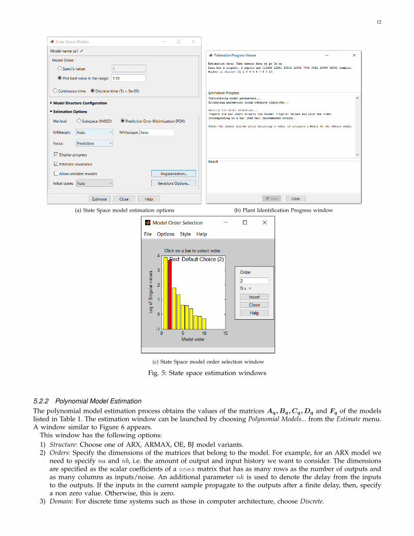
5.2.1 State Space Model EstimationThe state space model estimation process obtains the values of the matrices A, B, C, D and K (Equation 4) fromthe working set data. The estimation window can be launched by choosing the State Space Models... option inthe Estimate menu. A window similar to Figure 5a will be launched that presents the parameters for state spaceidentification. The parameters are as follows:

1) Model Order: The dimension of the model can be specified as a single value or, if we are not sure of thedimension of our system, a range of values. We specify the range 1:10. Choose a discrete time controller andverify the sampling time listed in the GUI with the sampling time of the data set.

2) Estimation Options: These list the different parameters for the identification algorithm. They are:a) Estimation Method: Typical choice is Prediction Error Minimization (PEM).b) Focus: Choose Prediction, if the final goal is to design a controller using the model, or choose Simulation

if we want to simulate a system.c) Allow unstable models: If the system under test is inherently stable – i.e., if the outputs do not steadily

reach extreme values (high or low) if the inputs to the system are not changed – then uncheck the Allowunstable models option.

Note that the designer can read and try other options for the parameters in state space estimation. After specifyingthe options, select Estimate. A Plant Identification Progress window (Figure 5b) and a Model Order Selection window(Figure 5c) will appear. If the Model Order was specified as a single value, only the former will appear. The chart inthe Model Order Selection window shows the contribution from each state. The red value shows the default selection.Usually, the impact of the states decreases after a certain order. The desired model order can be selected by clickingon the appropriate column in the chart or entering it in the Order: field. Click Insert to identify a model with thechosen order. This model will be inserted in the right-side pane of the system identification application. You candouble click on that icon to view its description, notes and options to rename it.

We estimate a state space model of order 4 for our data. We call this model ss4.

12

(a) State Space model estimation options

(b) Plant Identification Progress window

(c) State Space model order selection window

Fig. 5: State space estimation windows

5.2.2 Polynomial Model EstimationThe polynomial model estimation process obtains the values of the matrices Aq, Bq, Cq, Dq and Fq of the modelslisted in Table 1. The estimation window can be launched by choosing Polynomial Models... from the Estimate menu.A window similar to Figure 6 appears.

This window has the following options:1) Structure: Choose one of ARX, ARMAX, OE, BJ model variants.2) Orders: Specify the dimensions of the matrices that belong to the model. For example, for an ARX model we

need to specify na and nb, i.e. the amount of output and input history we want to consider. The dimensionsare specified as the scalar coefficients of a ones matrix that has as many rows as the number of outputs andas many columns as inputs/noise. An additional parameter nk is used to denote the delay from the inputsto the outputs. If the inputs in the current sample propagate to the outputs after a finite delay, then, specifya non zero value. Otherwise, this is zero.

3) Domain: For discrete time systems such as those in computer architecture, choose Discrete.

13

Fig. 6: Polynomial model estimation options

4) Focus: Select Stability if you are dealing with a stable system. Otherwise, choose Simulation.Click Estimate to insert the model with the specified parameters. This process has to be repeated multiple times

for estimating models of different orders.We estimate an ARX model with coefficients na = 2, nb = 2, nk = 0 and a BJ model with coefficients nb = 2, nc =

2, nd = 2, nf = 2, nk = 0. We call these models as arx22 and bj2222 respectively.

5.3 Model ValidationWe need to compare the set of models we estimated in the previous step, and pick the best model. The modelthat we identified should be able to isolate the deterministic parts of the system (influence of previous and currentinputs and previous outputs on current outputs) and the non-deterministic or noisy parts of the system (backgroundtasks, or other program behavior that affects outputs). This is the scale along which we judge the goodness of themodels.

For model comparison, it is recommended to use a data set that is different from the training and the deploymentdata sets. This process is called cross-validation. The data set that we want to use for model comparison should bein the Validation Data slot of the identification window. Then, select the models to be compared. A selected modelwill have thicker lines in the model icon. The selected models can be compared using the following metrics thatassess different aspects of a good model.

1) Simulation error: Difference between the output values given by the model, and the output values given bythe real system. In both cases, the inputs are the validation inputs.

2) Prediction error: This is the same as the simulation error, except that the model uses the values of the outputsfrom the real system as history, instead of the output values that the model generated in previous steps.

14

3) Residue characteristics: Ability of the model to explain the deterministic parts well.4) Frequency response: The behavior of the model when inputs are changing at different frequencies.

5.3.1 Simulation ErrorSelect the checkbox titled Model output under the models pane in the identification window to display the outputspredicted by the different models along with the true output. A Model Output window similar to Figure 7a willappear. The chart in this window shows the output values predicted by the models and the true output values (allfrom the validation data). Different output channels can be selected from the Channel menu. The pane titled BestFits: shows a metric for the quality of the fits. The values shown in this pane are not modeling errors. However,they are one way to assess the quality of the fit, with 100 indicating a perfect fit, 0 indicating a fit that is no betterthan a straight line at matching the real system data, and -Inf being the worst fit. You can use this to discard somemodels that are obviously bad. You might also want to change the type or order of the models based on theseresults. We can zoom inside the model output window to check if the models follow all the trends in the outputor not.

(a) Simulation error

(b) Confidence intervals for models

Fig. 7: Viewing simulation error

Instead of plotting the actual values of the model outputs, we can plot the instantaneous errors between themodeled and true outputs. The Error plot option from the Options menu displays the error signal instead of theactual signals.

In this experiment, we only feed the inputs (u(T )) to the model, and not the noise term (e(T ) = 0 in Equa-tions 4, 5, 6). As a result, the model outputs will not match the real system outputs exactly. However, the modeloutputs should be able to follow all the trends in the real system outputs. Therefore, it means that the model is ableto capture the dynamics of the deterministic parts of the system. In the step titled Residue characteristics, we willensure that the difference between the model output and the real system output does not have any deterministiccomponents, and is purely white noise – i.e., random.

We can also see how likely it is for the deterministic output of the system to be near the deterministic output ofthe model. This is done through confidence levels and intervals. A confidence interval is a range around the modeloutput within which the true output is contained with a probability specified by the confidence level. A higherconfidence level means that we want to be more sure of where the true output is. Therefore, this will correspondto a larger region around the model output, resulting in a larger confidence interval. An extreme case is if we wantto have a confidence level of 100% on the location of the true outputs, then the confidence interval is the entirepossible output value space. A confidence level of 99% spans three standard deviations and is commonly used.The confidence levels can be specified and the intervals can be displayed by selecting appropriate options from theOptions menu. The boundaries appear as dashed lines and you might need to zoom in the plot to view them. Forgood models, the confidence intervals lie close to the nominal model output, even with > 99% confidence levels.Figure 7b shows the confidence intervals for different models for the output corresponding to power.

15

5.3.2 Prediction ErrorPrediction is the same as simulation except that, to compute the current output values, the model uses the truevalues of previous outputs instead of the previous output values given by the model. We can also specify howmuch ahead the model needs to predict the output. We can set this look-ahead value and show the predictionresults by choosing the corresponding options from the Options menu.

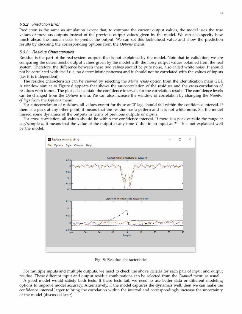
5.3.3 Residue CharacteristicsResidue is the part of the real-system outputs that is not explained by the model. Note that in validation, we arecomparing the deterministic output values given by the model with the noisy output values obtained from the realsystem. Therefore, the difference between these two values should be pure noise, also called white noise. It shouldnot be correlated with itself (i.e. no deterministic patterns) and it should not be correlated with the values of inputs(i.e. it is independent).

The residue characteristics can be viewed by selecting the Model resids option from the identification main GUI.A window similar to Figure 8 appears that shows the autocorrelation of the residues and the cross-correlation ofresidues with inputs. The plots also contain the confidence intervals for the correlation results. The confidence levelscan be changed from the Options menu. We can also increase the window of correlation by changing the Numberof lags from the Options menu.

For autocorrelation of residues, all values except for those at ‘0’ lag, should fall within the confidence interval. Ifthere is a peak at any other point, it means that the residue has a pattern and it is not white noise. So, the modelmissed some dynamics of the outputs in terms of previous outputs or inputs.

For cross correlation, all values should lie within the confidence interval. If there is a peak outside the range atlag/sample k, it means that the value of the output at any time T due to an input at T − k is not explained wellby the model.

Fig. 8: Residue characteristics

For multiple inputs and multiple outputs, we need to check the above criteria for each pair of input and outputresidue. These different input and output residue combinations can be selected from the Channel menu as usual.

A good model would satisfy both tests. If these tests fail, we need to use better data or different modelingoptions to improve model accuracy. Alternatively, if the model captures the dynamics well, then we can make theconfidence interval larger to bring the correlation within the interval and correspondingly increase the uncertaintyof the model (discussed later).

16

5.3.4 Frequency ResponseThe outputs of the system may be influenced by the rate of change of inputs. For example, consider the impact ofcache size on performance. When the cache size is decreased, performance drops suddenly but regains some of itslost performance as the frequently-used values accumulate in the smaller cache. If the size of the cache is going tochange again before the earlier performance transient settles, the impact could be higher/lesser than what could beexpected otherwise. On the other hand, consider the case of frequency and power. Once a particular frequency ischosen, the power of the system varies immediately and there is no change once the power moves to a new value,unlike the previous example. Frequency response is a way to understand how the impact of the inputs on theoutputs varies with the rate of change of inputs. This information can be viewed using the Frequency resp checkboxin the identification GUI.

Figure 9 shows the frequency response of the models we identified for the pair u1→y1 – i.e., cache size to IPS.Note that both axes are logarithmic. The chart shows the magnitude of impact of the input on the output as thefrequency of the input is changed. In this chart, the input-output pairs can be selected from the Channel menu.For input-output pairs where the rate of change of input matters, the frequency response curve should changeaccordingly. For other pairs, such as the effect of frequency on power, the curve should be nearly flat.

Fig. 9: Evaluating the frequency response of different models

We can customize the frequency range by specifying the desired range in the Frequency range... dialog of theOptions menu. A helpful MATLAB command for describing frequency ranges is logspace. We can also changethe axes limits or switch from log to linear scale using the Set axes limits... dialog box from the Options menu. Theseare useful to view the behavior of the model at frequencies of interest to the designer.

The frequency response chart can also be annotated with confidence intervals, using the Options menu as before.The width of the confidence intervals can be used to estimate uncertainties, as will be described in the next section.

5.4 Uncertainty EstimationOne way to view uncertainty can be seen in Figure 10 where the dark line shows the frequency response of themodel, the shaded region represents the dynamics within the uncertianty limits and the dotted line shows the truefrequency response of the system. We use the information from the nominal model and design a controller to workfor all possible dynamics within the shaded region.

Frequency

Magnitude

Fig. 10: Understanding Uncertainty

17

The uncertainty guardband we decide is not directly used for designing the LQG controller. Instead it is used tocheck the robustness of the LQG controller we design (Figure 2). Robust Stability Analysis takes this uncertaintyguardband we specify and tests whether the design is stable even if the model deviates from the true systemconsistently by at most the specified guardband. This can ascertain that the final controller we design is applicablefor a large set of scenarios and does not create unexpected behavior.

It is recommended to use challenging applications to validate the model performance and estimate uncertainty.Specifying a larger uncertainty means that the final controller is stable for a large region and can tolerate modelvariations. However, needlessly specifying a very large uncertainty can result in an extremely slow controller. Thereare many ways to estimate the uncertainty of the model, some of which we discuss here.

1) Simulation error: We consider the error between the true and model outputs to specify a certain uncertainty.This is similar to the model validation step with the same name except that we also excite the noise componentsof the system. We will use the error between the model output and the validation data to compute differentaccuracy measures. These measures could be the ratio of the maximum error value to the mean error value,or the maximum ratio of the error value to the model output value, or any such relevant metric. This measurecan be used as an uncertainty estimate.

2) Parametric uncertainty: MATLAB can also specify the uncertainties of the values in the model that it identified.Double click on a model to bring up the Data/Model Info window and select Present or use the commandpresent to list the identified parameters and their uncertainties in the MATLAB workspace. This uncertaintyneeds to be converted to a form called multiplicative uncertainty, which is then used to determine theuncertainty bounds. More information on performing this conversion with an example can be seen in [14].

3) Model error model: In this method, we identify a secondary model between the model error and the inputsfrom the validation data. This secondary model has more reliable information about the uncertainty boundsof the original model. This is more complicated than the other steps but can provide accurate uncertaintybounds. More information can be obtained from [15].

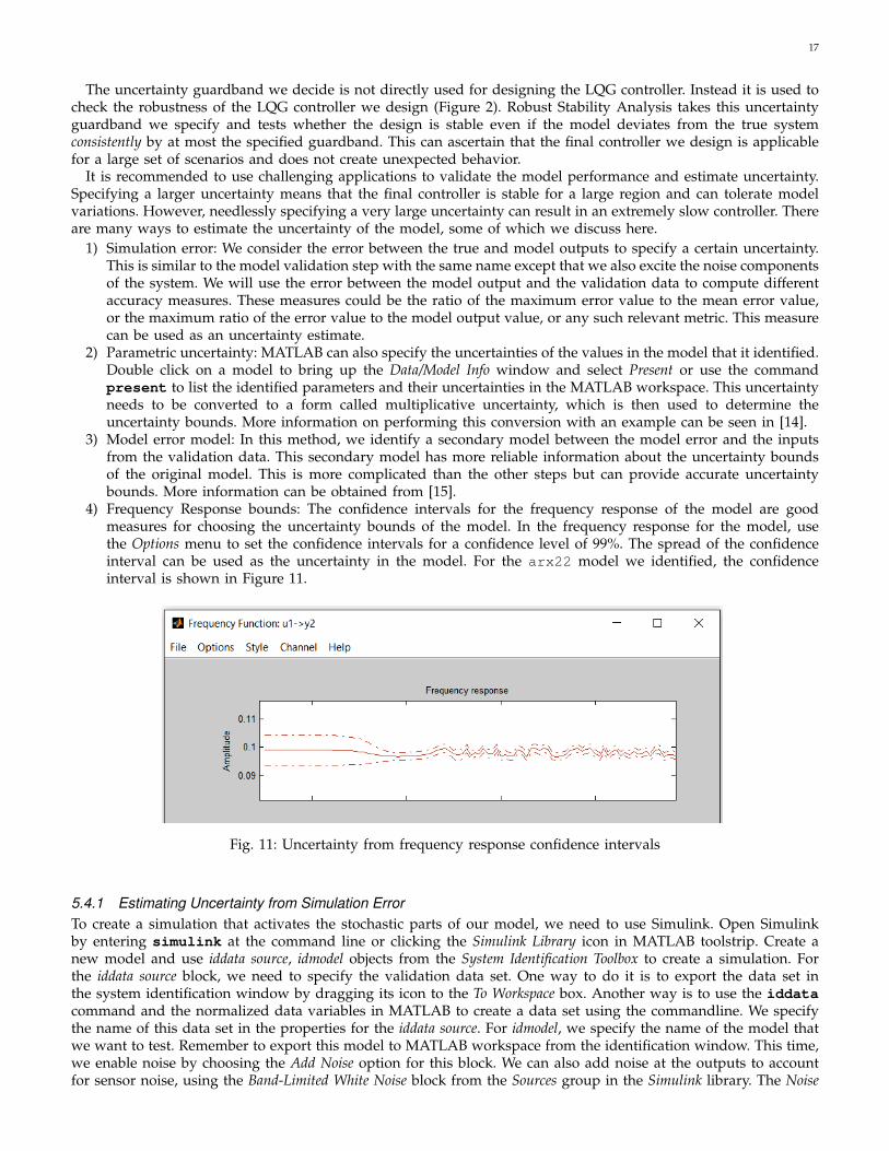
4) Frequency Response bounds: The confidence intervals for the frequency response of the model are goodmeasures for choosing the uncertainty bounds of the model. In the frequency response for the model, usethe Options menu to set the confidence intervals for a confidence level of 99%. The spread of the confidenceinterval can be used as the uncertainty in the model. For the arx22 model we identified, the confidenceinterval is shown in Figure 11.

Fig. 11: Uncertainty from frequency response confidence intervals

5.4.1 Estimating Uncertainty from Simulation ErrorTo create a simulation that activates the stochastic parts of our model, we need to use Simulink. Open Simulinkby entering simulink at the command line or clicking the Simulink Library icon in MATLAB toolstrip. Create anew model and use iddata source, idmodel objects from the System Identification Toolbox to create a simulation. Forthe iddata source block, we need to specify the validation data set. One way to do it is to export the data set inthe system identification window by dragging its icon to the To Workspace box. Another way is to use the iddatacommand and the normalized data variables in MATLAB to create a data set using the commandline. We specifythe name of this data set in the properties for the iddata source. For idmodel, we specify the name of the model thatwe want to test. Remember to export this model to MATLAB workspace from the identification window. This time,we enable noise by choosing the Add Noise option for this block. We can also add noise at the outputs to accountfor sensor noise, using the Band-Limited White Noise block from the Sources group in the Simulink library. The Noise

18

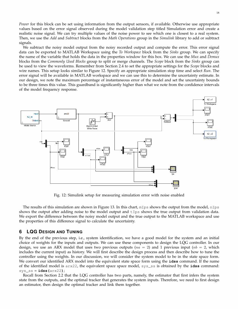
Power for this block can be set using information from the output sensors, if available. Otherwise use appropriatevalues based on the error signal observed during the model validation step titled Simulation error and create arealistic noise signal. We can try multiple values of the noise power to see which one is closest to a real system.Then, we use the Add and Subtract blocks from the Math Operations group in the Simulink library to add or subtractsignals.

We subtract the noisy model output from the noisy recorded output and compute the error. This error signaldata can be exported to MATLAB Workspace using the To Workspace block from the Sinks group. We can specifythe name of the variable that holds the data in the properties window for this box. We can use the Mux and Demuxblocks from the Commonly Used Blocks group to split or merge channels. The Scope block from the Sinks group canbe used to view the waveforms. Remember from Section 2.4 to set the appropriate settings for the Scope blocks andwire names. This setup looks similar to Figure 12. Specify an appropriate simulation stop time and select Run. Theerror signal will be available in MATLAB workspace and we can use this to determine the uncertainty estimate. Inour design, we note the maximum percentage of instantaneous error of the model and set the uncertainty boundsto be three times this value. This guardband is significantly higher than what we note from the confidence intervalsof the model frequency response.

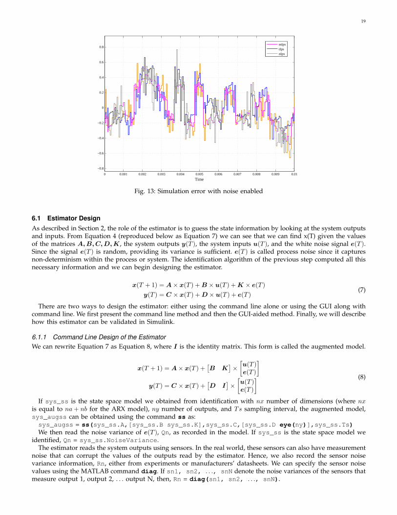
Fig. 12: Simulink setup for measuring simulation error with noise enabled

The results of this simulation are shown in Figure 13. In this chart, mIps shows the output from the model, nIpsshows the output after adding noise to the model output and tIps shows the true output from validation data.We export the difference between the noisy model output and the true output to the MATLAB workspace and usethe properties of this difference signal to calculate the uncertainty.

6 LQG DESIGN AND TUNING

By the end of the previous step, i.e., system identification, we have a good model for the system and an initialchoice of weights for the inputs and outputs. We can use these components to design the LQG controller. In ourdesign, we use an ARX model that uses two previous outputs (na = 2) and 1 previous input (nb = 2, whichincludes the current input) as history. We will first describe the design process and then describe how to tune thecontroller using the weights. In our discussion, we will consider the system model to be in the state space form.We convert our identified ARX model into the equivalent state space form using the idss command. If the nameof the identified model is arx22, the equivalent space space model, sys_ss is obtained by the idss command:sys_ss = idss(arx22);

Recall from Section 2.2 that the LQG controller has two parts, namely, the estimator that first infers the systemstate from the outputs, and the optimal tracker that generates the system inputs. Therefore, we need to first designan estimator, then design the optimal tracker and link them together.

19

0 0.001 0.002 0.003 0.004 0.005 0.006 0.007 0.008 0.009 0.01

−0.8

−0.6

−0.4

−0.2

0

0.2

0.4

0.6

0.8

Time

mIpstIpsnIps

Fig. 13: Simulation error with noise enabled

6.1 Estimator DesignAs described in Section 2, the role of the estimator is to guess the state information by looking at the system outputsand inputs. From Equation 4 (reproduced below as Equation 7) we can see that we can find x(T) given the valuesof the matrices A, B, C, D, K, the system outputs y(T ), the system inputs u(T ), and the white noise signal e(T ).Since the signal e(T ) is random, providing its variance is sufficient. e(T ) is called process noise since it capturesnon-determinism within the process or system. The identification algorithm of the previous step computed all thisnecessary information and we can begin designing the estimator.

x(T + 1) = A× x(T ) + B × u(T ) + K × e(T )y(T ) = C × x(T ) + D × u(T ) + e(T )

(7)

There are two ways to design the estimator: either using the command line alone or using the GUI along withcommand line. We first present the command line method and then the GUI-aided method. Finally, we will describehow this estimator can be validated in Simulink.

6.1.1 Command Line Design of the EstimatorWe can rewrite Equation 7 as Equation 8, where I is the identity matrix. This form is called the augmented model.

x(T + 1) = A× x(T ) +[B K

]×

[u(T )e(T )

]y(T ) = C × x(T ) +

[D I

]×

[u(T )e(T )

] (8)

If sys_ss is the state space model we obtained from identification with nx number of dimensions (where nxis equal to na + nb for the ARX model), ny number of outputs, and Ts sampling interval, the augmented model,sys_augss can be obtained using the command ss as:sys_augss = ss(sys_ss.A,[sys_ss.B sys_ss.K],sys_ss.C,[sys_ss.D eye(ny)],sys_ss.Ts)We then read the noise variance of e(T ), Qn, as recorded in the model. If sys_ss is the state space model we

identified, Qn = sys_ss.NoiseVariance.The estimator reads the system outputs using sensors. In the real world, these sensors can also have measurement

noise that can corrupt the values of the outputs read by the estimator. Hence, we also record the sensor noisevariance information, Rn, either from experiments or manufacturers’ datasheets. We can specify the sensor noisevalues using the MATLAB command diag. If sn1, sn2, . . ., snN denote the noise variances of the sensors thatmeasure output 1, output 2, . . . output N, then, Rn = diag(sn1, sn2, . . ., snN).

20

If there is sensor noise but we do not know any information about it, the GUI method described later can beused to find out this information. If there is no sensor noise, this value is zero (Rn = zeros(ny)). Sometimes, theunderlying algorithms can flag an error when Rn is specified as zero. In such cases use a small non zero value suchas 1e-6 (i.e., Rn = 1e-6*eye(ny)).

We then build the estimator, Kest, using the augmented model and the noise variance values using the kalmancommand. Kest = kalman(sys_augss, Qn, Rn).

Enter the name of the estimator, Kest, in the workspace to view information about the estimator. Note the orderof inputs in the Input groups: field. The Output groups: field lists the order of the output estimates andstate estimates.

We can test the estimator in Simulink even before testing it on the real system. There are two ways to test theestimator. In the first, we use the model to generate clean output, add noise to it and check the output predictedby the estimator as well as the true output. In the second way, we add noise to the validation data directly, andcompare the output predicted by the estimator to the validation output. These two setups are shown in Figures 14and 15 respectively.

Fig. 14: Simulink setup for validating the estimator using model outputs

Fig. 15: Simulink setup for validating the estimator using validation outputs

Use the Iddata Source, Idmodel from the System Identification Toolbox to setup a simulation as before. Use a Band-Limited White Noise block from the Sources group in the Simulink library to add noise to the output signal (eithervalidation output or model output). Specify the noise power to resemble a realistic scenario. Add an LTI Systemblock from the Control System Toolbox. This will function as the estimator. Specify the name of the estimator wedesigned, Kest, in the properties of this block. The input channel to this estimator consists of known inputs and

21

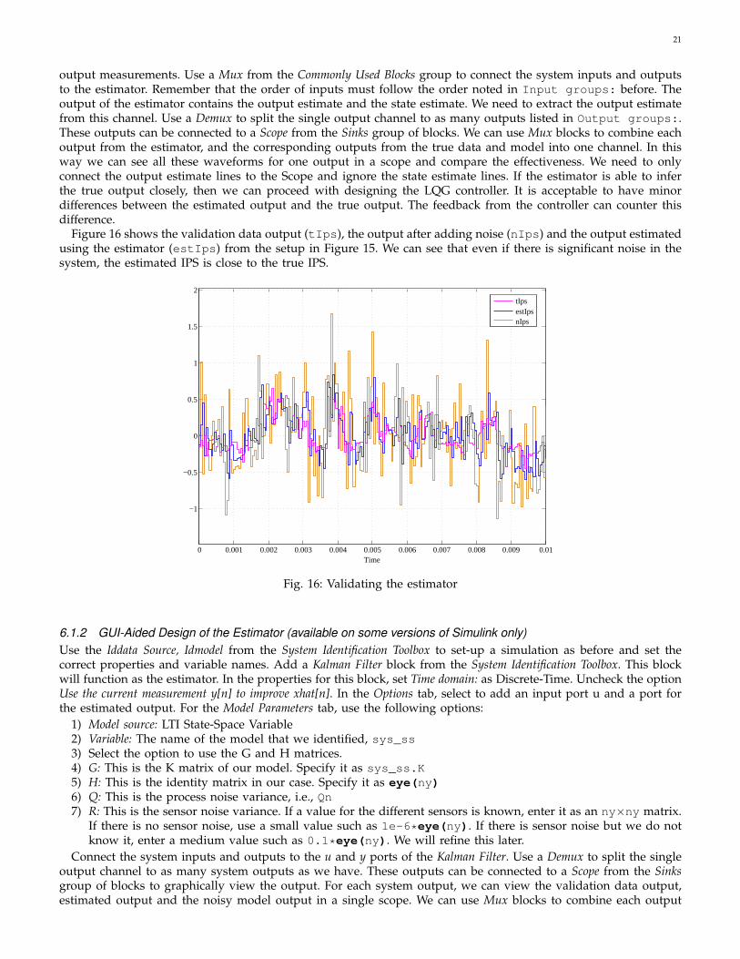
output measurements. Use a Mux from the Commonly Used Blocks group to connect the system inputs and outputsto the estimator. Remember that the order of inputs must follow the order noted in Input groups: before. Theoutput of the estimator contains the output estimate and the state estimate. We need to extract the output estimatefrom this channel. Use a Demux to split the single output channel to as many outputs listed in Output groups:.These outputs can be connected to a Scope from the Sinks group of blocks. We can use Mux blocks to combine eachoutput from the estimator, and the corresponding outputs from the true data and model into one channel. In thisway we can see all these waveforms for one output in a scope and compare the effectiveness. We need to onlyconnect the output estimate lines to the Scope and ignore the state estimate lines. If the estimator is able to inferthe true output closely, then we can proceed with designing the LQG controller. It is acceptable to have minordifferences between the estimated output and the true output. The feedback from the controller can counter thisdifference.

Figure 16 shows the validation data output (tIps), the output after adding noise (nIps) and the output estimatedusing the estimator (estIps) from the setup in Figure 15. We can see that even if there is significant noise in thesystem, the estimated IPS is close to the true IPS.

0 0.001 0.002 0.003 0.004 0.005 0.006 0.007 0.008 0.009 0.01

−1

−0.5

0

0.5

1

1.5

2

Time

tIpsestIpsnIps

Fig. 16: Validating the estimator

6.1.2 GUI-Aided Design of the Estimator (available on some versions of Simulink only)Use the Iddata Source, Idmodel from the System Identification Toolbox to set-up a simulation as before and set thecorrect properties and variable names. Add a Kalman Filter block from the System Identification Toolbox. This blockwill function as the estimator. In the properties for this block, set Time domain: as Discrete-Time. Uncheck the optionUse the current measurement y[n] to improve xhat[n]. In the Options tab, select to add an input port u and a port forthe estimated output. For the Model Parameters tab, use the following options:

1) Model source: LTI State-Space Variable2) Variable: The name of the model that we identified, sys_ss3) Select the option to use the G and H matrices.4) G: This is the K matrix of our model. Specify it as sys_ss.K5) H: This is the identity matrix in our case. Specify it as eye(ny)6) Q: This is the process noise variance, i.e., Qn7) R: This is the sensor noise variance. If a value for the different sensors is known, enter it as an ny×ny matrix.

If there is no sensor noise, use a small value such as 1e-6*eye(ny). If there is sensor noise but we do notknow it, enter a medium value such as 0.1*eye(ny). We will refine this later.

Connect the system inputs and outputs to the u and y ports of the Kalman Filter. Use a Demux to split the singleoutput channel to as many system outputs as we have. These outputs can be connected to a Scope from the Sinksgroup of blocks to graphically view the output. For each system output, we can view the validation data output,estimated output and the noisy model output in a single scope. We can use Mux blocks to combine each output

22

from the estimator, and the corresponding outputs from the true data and model into one channel. To accountfor sensor noise, use a Band-Limited White Noise block from the Sources block and add this to the system output.Connect this noisy output to the Kalman filter instead of connecting the system output directly. Remember to seta realistic Noise Power for the noise. If the estimator is able to infer the true output closely, then we can use thekalman command as before to design the estimator with the Rn values that we specified. Otherwise, we can refinethe value of Rn until we see satisfactory estimator quality, and then use that value for designing the estimator. Itis acceptable to have minor differences between the estimated output and the true output.

6.2 Optimal Tracker and LQG Controller DesignAfter the estimator design, we need to design an optimal tracking controller and link the estimator with the tracker.The tracker uses the state estimate from the estimator along with output tracking errors to generate the systeminputs.

To design the tracking controller, we only need the deterministic part of the model and the weights that wedecided for the inputs and outputs. Use the ss command to specify the state space form of the deterministiccomponents of our model, sys_ss:sys_detss = ss(sys_ss.A,sys_ss.B,sys_ss.C,sys_ss.D,sys_ss.Ts);We need to augment the output weight matrix with what are called state weights for the estimated states that

are supplied by the estimator. In our case, we are interested in output tracking and can set these weights to zeroor a small value. If Q is the diagonal matrix of weights for the outputs, and nx is the number of states (dimension)of the state space model sys_ss, the augmented weights matrix, Qa, is obtained using the following command:Qa = blkdiag(0*eye(nx),Q);Using Qa and the diagonal input weight matrix, R, we can design the optimal tracker, Ktrk, using the lqi

command as follows:Ktrk = lqi(sys_detss, Qa, R);Finally we link the optimal tracker and the estimator to generate the optimal controller, Klqg, using the lqgtrack

command:Klqg = lqgtrack(Kest,Ktrk,‘1dof’);The ‘1dof’ argument in this command is specifying that the input to the controller will be the output tracking

error. If this argument is not specified or if the alternative argument ‘2dof’ is specified, the input to the controllerwill be the output reference values directly.

We can type the name of the LQG controller we designed, Klqg, at the command line to view the four matricesa, b, c, d that constitute the controller. The controller takes the output tracking errors, y(T ), and produces thechanges to be applied to the inputs, u(T ). It uses a state variable x(T ) to store the internal information. Thesevalues are related as shown in Equation 9.

x(T + 1) = a× x(T ) + b× y(T )u(T ) = c× x(T ) + d× y(T )

(9)

When using the controller, we perform these matrix vector multiplications to determine the changes to the systeminputs and the next state.

6.3 LQG TuningBefore deploying the controller, we can test and, if necessary, tune the characteristics of the controller. There aretwo phases in LQG Tuning. The first is to check whether the controller is converging fast enough and whether theripples are acceptable. The second is to ensure robust stability. We can perform the first phase using Simulink, andthis process is described here.

Setup a Simulink model with two LTI System blocks from the Control System Toolbox. One of them will be thesystem model, sys_ss, and the other will be the controller, Klqg. Connect the controller to the system model.Use a Constant block from the Sources group to create the reference values for each output. With multiple outputs,we might need to use a Mux and combine the different reference signals. Connect this reference signal to a Sumblock from the Commonly Used Blocks group. The output from the system model should be connected to the otherinput port of the Sum block. Ensure that the Sum block is performing the operation r(T )−y(T ), where r(T ) is thereference signal and y(T ) is the system output. Connect the output of the Sum block to the controller. Use multipleDemux and Scope blocks to view the different signals. When we run the simulation, we can see the behavior ofthe system and the controller from the input and output waveforms. If we find that the system is taking too longto reach the reference values, we can resynthesize the tracker with a higher weight for outputs relative to inputs

23

Fig. 17: Simulink setup for tuning the LQG controller (normalized signals)

(Section 3). Similarly, if we find that the system is too ripply, we can reduce the weights of the outputs relative tothe inputs. The setup is similar to Figure 17.

Note that in this simulation, the input and output changes are on a normalized scale, since we applied normal-ization to the original data. We can use Gain blocks from the Commonly Used Blocks group and Add, Subtract blocksfrom the Math Operations group to re-scale the values before viewing them. If scaling was applied according toEquation 3, we can rewrite it as Equation 10.

Vnew =Vold

S+ O; where S =

Vmin − Vmin

2, O = −Vmax + Vmin

Vmax − Vmin

Vold = S × (Vnew −O)(10)

If S is the scaling factor, the gain value to be used to re-scale the signals is S. In the Multiplication options for theGain blocks, choose Matrix(K*u). For channels carrying multiple inputs or outputs, specify the gain as a diagonalmatrix with the re-scaling factor for each individual signal along the corresponding diagonal entry.

We can modify the Simulink model to include the other aspects of the system, such as input quantization (inputstake discrete values) and saturation (inputs take finite number of values). The Quantizer and Saturation blocks fromthe Discontinuities group perform these actions. We can re-scale the inputs as mentioned earlier, pass them throughthe Quantizer and Saturation blocks, scale them again using a gain block with 1

S and feed that input to the system.We can test if the performance of the controller is acceptable after imposing these constraints. The Simulink modeldiagram that includes these blocks in addition to the re-scaled signals is similar to Figure 18. In some versionsof Simulink, if the d matrix of the controller (i.e., Klqg) is non-zero, then adding blocks from the Discontinuitiestoolbox may cause an error. In such scenarios, one can only use re-scaling to make sure inputs are within saturationlimits in Simulink. The controller can be tuned on the actual system instead of using Simulink. A work around isto use another temporary controller that has the same a, b, c matrices as Klqg but the d matrix is 0. In this case,we need to check if the temporary controller is also stabilizing the system before simulation, using the loopsenscommand. For example, this could be done through the following code snippet:tmplqgCtl = Klqg;tmplqgCtl.d = zeros(ny,nu);loopsens(sys_ss,tmplqgCtl);

In this code, nu is the number of system inputs (or controller outputs). The loopsens displays a set of entriesof which the Stability field should have the value 1. Then, the system with the temporary controller is stable.Remember to use this temporary controller only for simulation and not for deployment.

Figure 19 shows how the IPS and power of the system moves from an initial value of 0 to the targets that wespecify – 1W for power and 0.5 BIPS for IPS. We could further tune the input and output weights to change thecharacteristics of the controller such as the rate of convergence or transient overshoots. The minor oscillations aftersteady state are due to the quantization in the allowable input values. In scenarios where an intermediate value isneeded to make the outputs reach the references exactly, the controller choice might waver between the two levelsthat contain the intermediate value.

7 ROBUSTNESS ANALYSIS

Robust controller design is a well-studied area in Control Theory. In this area, the system model used in the designof the controller is called the nominal model. Such model is different from the real system. All unaccounted factors,

24

Fig. 18: Simulink setup for tuning the LQG controller (de-normalized signals)

0 0.001 0.002 0.003 0.004 0.005 0.006 0.007 0.008 0.009 0.01

−0.1

0

0.1

0.2

0.3

0.4

0.5

0.6

Time

IPS

ips

(a) IPS

0 0.001 0.002 0.003 0.004 0.005 0.006 0.007 0.008 0.009 0.01

0

0.2

0.4

0.6

0.8

1

1.2

Time

Pow

er

pow

(b) Power

Fig. 19: Testing the LQG controller in Simulink

modeling simplifications, and modeling limitations are what is called model uncertainties. In this case, a systemcan be represented schematically as in Figure 20. The goal of robust controller design is to ensure that the controlleris stable for all the uncertainties whose maximum sustained impact is bounded by a designer-specified margin.

Robust

Controller

Nominal

Model+__

Uncertainty

Target

oy (T) error

y(T) u(T) y(T)

System

Fig. 20: Uncertainty and nominal system model

In Figure 20, the uncertain dynamics are shown to modify the system dynamics in an unknown way. The controllerwe design should work correctly as long as these perturbations are bounded by a certain uncertainty margin. Inour case, these bounds are the uncertainty limits we estimated during System Identification (Section 5.4). The realsystem might deviate from the model or have non-linearities or other effects that might not be modeled, but aslong as they are within the limits, the robust controller will not have a problem in stabilizing the system. Theidea of a robust controller is better understood by re-drawing Figure 20 as Figure 21a. In Figure 21a, we have anaugmented uncertain system that has bounded unknown dynamics shown as ∆, and the controller is interactingwith this augmented system. Wr is the percentage of uncertainty in the system; zr is the disturbance signal.

Another way to look at this structure is shown in Figure 21b. In this figure, we have a closed loop system consistingof the system and the controller. There are unknown dynamics that are interfering with the controller actions. Theidea of robust control is that if the path from zr to wr (i.e., the system without the uncertainty component) does

25

Nominal

Model

y(T)u(T)

System

Robust

Controller

rWrw rz

++

(a)

Nominal

Model

y(T)u(T)

Closed loop

system

Robust

Controller

rWrw rz

++

(b)

Fig. 21: Understanding robust control

not magnify the disturbance signal zr, then whatever the ∆ block might do, the disturbance can never increasesuch that the system destabilizes. The controller design is such that it is prepared enough to withstand Wr fractionof uncertainty, and as long as the disturbance is within this fraction, it can keep the system stable.

Robustness analysis is a very conservative analysis because it assumes that the worst form of uncertainty is actingin the worst manner, from the beginning of the system operation, with a single dedicated purpose to destabilizethe system. While such scenarios can be thought of theoretically, they occur rarely in practice.

The first step to perform robustness analysis is to define the uncertainty limits. Then, we describe the connectionsbetween the blocks as in Figure 21. Finally, we perform the robustness test to check whether our controller canstabilize the uncertain model robustly or not.

7.1 Specifying Uncertainty GuardbandsMATLAB allows specifying an uncertainty limit that is dependent on the rate of change of inputs. For example, insome scenarios, we may have accurate models when the inputs are changing slowly (order of ms), but the accuracymay not be high when the inputs are changing very fast (µ s). In that case, we can specify a lower uncertainty forslow changes and a high uncertainty for fast changes. In our case, we assume that the same uncertainty occurs forall rates of change. We define this uncertainty in each of the outputs using transfer functions (Section 2.5). The gainof the transfer function at each frequency represents the model uncertainty for an output when inputs are changingwith that frequency. In this paper, the fixed uncertainties that we use for IPS and power are 50% and 30% at allrates of input changes. Hence, we use the transfer functions, Wri = 0.5 and Wrp = 0.3 to represent this modeluncertainty. These can be defined using the nd2sys command:Wri = nd2sys([0 1],[0 1],0.5);Wrp = nd2sys([0 1],[0 1],0.3);We combine these two blocks into one uncertainty block using the daug command:Wr = daug(Wri, Wrp);We need to discretize this transfer function since we are dealing with a discrete-time system. We use the samhld

function that takes the sampling interval, Ts, as a parameter:Ts = 5e-5;Wrd = samhld(Wr, Ts);The frequency response of this transfer function, Wr g, can be calculated using the frsp command. This command

also requires the set of frequencies for which we want to calculate the response. This range can be generated usingthe logspace command:frange = logspace(4,10,100);This command generates 100 points between 104 and 1010. These can be changed to suit the frequencies of interest

to the designer. We can then calculate the frequency response as follows:Wr_g = frsp(Wr_f,frange,Ts);To plot this function, we use the vplot command. More options for this command can be found by using help

vplot at the commandline.vplot(‘liv,m’,Wr_g);This shows a plot similar to Figure 22. In the figure, Wri shows the percentage of uncertainty in the first output

(i.e., IPS) and Wrp shows the percentage of uncertainty in the second output (i.e., power).

26

104

105

106

107

108

109

0

0.1

0.2

0.3

0.4

0.5

0.6Multiplicative Uncertainty Weighting Function

Frequency (rad/s)

Mag

nitu

de

W

ri

Wrp

Fig. 22: Frequency response of the transfer functions that represent uncertainty in outputs

7.2 Specifying the Augmented Uncertain SystemSince we will be using the Robust Control Toolbox commands to perform the robustness test, we need to representthe nominal system in the required format, and then describe the augmented system. A state space model withmatrices A,B, C, D needs to be represented in a packed format as shown in Figure 23.

A B

C D

Fig. 23: Packed format of systems to use robust control toolbox commands

The packed format (PM) for the nominal system model sys_ss is obtained through the pck command as follows:PM = pck(sys_ss.A, sys_ss.B, sys_ss.C, sys_ss.D);We also need to represent the controller we designed, Klqg, in the packed format (KlqgM):KlqgM = pck(Klqg.A, Klqg.B, Klqg.C, Klqg.D);We can describe the augmented system of Figure 21 using the sysic set of commands. In this method, we list

the components of the augmented system, then list all its input and output signals, and then specify the connectionsto each block within the augmented system. The output signal names are specified by specifying the names of theblocks that generate the output signals. The ∆ block need not be explicitly specified. We will also add the controllerto the terminals of the uncertain system later. Therefore, we specify all remaining connections except the controllerand ∆ blocks of Figure 21 in this step. This set of connections are shown as the part called PMOL in Figure 24.

In this figure, the controller is given the symbol, K. The system output is multiplied by −1 because the controllertakes in y◦(T )−y(T ), i.e., the system output is subtracted form the reference outputs. The connections are specifiedin MATLAB using the following code fragment:systemnames = ’ PM Wr ’;inputvar = ’[ zr_{2} ; ctl{2}]’; % there are two uncertain output channels and

; % two channels for the controller outputoutputvar = ’[ Wr ; -PM ]’; % minus sign because of feedbackinput_to_PM = ’[ ctl + zr_ ]’;input_to_Wr = ’[ ctl ]’;sysoutname = ’PMOL’;cleanupsysic = ’yes’;sysic;

27

PM

PMOL

Klqg

Wr

++

ctl

zr

-1

Fig. 24: Describing the connections of the open loop system using sysic

The name of the augmented system is PMOL. We will now connect the controller to this augmented systemand build the closed loop system, clpic, using the starp command. If the controller can take ny inputs, then,MATLAB ensures that the last ny signals of outputvar are connected to the controller when this command isused. In our case, the last two outputvar (i.e., the nominal system outputs) are connected to the controller.clpic = starp((PMOL, KlqgM);

7.3 Performing the Robustness TestRobust stability is tested by calculating the frequency response of the closed loop system. The gain of the augmentedsystem should be smaller than 1. That means that our system is robustly stable. We use the frsp command asbefore to obtain the frequency response:clpic_g = frsp(clpic,2*pi*frange,Ts);We select the response between the first two inputs (zr) and the first two outputs (wr) for the augmented system

using the sel command, and the magnitude is plotted using the vplot command:rob_stab = sel(clpic_g,[1 2],[1 2]);vplot(’liv,m’,vnorm(rob_stab));From this plot, we need to ensure that the frequency response is smaller than 1 for all the frequencies of interest.

If not, then we need to either change the weights appropriately (i.e., decrease output weights relative to the inputweights) or change the model to obtain smaller guardbands. Figure 25 shows the robustness of the controller wedesigned. The figure shows, for different frequencies, the absolute value of TFzw — i.e., the transfer function fromzr to wr. Recall that we said that the gain from zr to wr should be less than 1. Therefore, the absolute value ofTFzw should be less than 1.

If we find any issues in robustness, we need to re-visit one or more steps in the LQG design flow. If we aresatisfied with the behavior of the controller and its robustness, we are done and we can deploy the controller inthe real system.

APPENDIX: DESIGNING HEURISTIC ALGORITHMS

In this appendix, we describe in detail the heuristic algorithms outlined in [1]. Note that there are many heuristicalgorithms from prior work that change a single architectural parameter to meet a single output objective. However,it is not straightforward to combine multiple such algorithms to change several architectural parameters to meetseveral output objectives. Such combination may cause the benefits of each individual algorithm to vanish. Due toa lack of coordinated heuristic policies that change multiple parameters to achieve multiple output objectives, webuild our own custom heuristic algorithms. We build two of them.

28

104

105

106

107

108

109

1010

1011

0.4

0.5

0.6

0.7

0.8

0.9

1Robust Stability Analysis of Klqg

Frequency (rad/s)

|TF zw

|

Fig. 25: Robust Stability Analysis of our LQG controller

Heuristic Tracking AlgorithmOur first heuristic algorithm changes two inputs (cache size and processor frequency) to track two output objectives(application instructions per second or IPS, and processor power). We will compare the effectiveness of this heuristictracking algorithm to our control-theoretic MIMO approach. The heuristics algorithm operates in two stages. Thefirst stage ranks the inputs based on the magnitude of their impact on the outputs. The second stage uses thisinformation, along with the output tracking error, to dynamically determine how to change the inputs. This schemeis similar to the heuristic scheme in [16].

In the first stage, we consider the impact of our two inputs on the application IPS. During memory-intensiveapplication phases, the cache size has a higher impact than the frequency on the IPS; during compute-intensivephases, the frequency has a higher impact than the cache size on IPS. We also note that, generally, increases inIPS tend to go together with increases in processor power, and decreases in IPS imply decreases in processorpower. Hence, we periodically measure the ratio of the number of memory instructions over the total number ofinstructions (Mem

µOp ), similarly to [17]. Then, in application phases where MemµOp is high, we log cache size as the more

important input (Inphigh) and frequency as the less important one (Inplow). In phases where MemµOp is low, frequency

is Inphigh and cache size is Inplow. If we had more inputs, we would need to rank-order all of them as in [16].In a given application phase, we define the IPS tracking error (eIPS) as the target IPS value (IPS0) minus the

current IPS value; we define the power tracking error (ePower) as the target power value (Power0) minus the currentpower value. With these definitions, a positive error means that the output value is lower than the target value, andwe need to increase the inputs; a negative error means that the output value is higher than the target value, andwe need to lower the inputs. If the output value is within the tolerance margin around the reference, we considerthe error to be zero.

In the second stage of our heuristic tracking algorithm, we dynamically decide on how to change Inphigh andInplow based on the magnitude and sign of the output tracking errors. Since we have two outputs, we can have ninepossible combinations of the tracking error signs. For example, eIPS may be positive while ePower may be zero. Formost of these scenarios, we can have different magnitudes of error. For example, eIPS may have a large positivemagnitude while ePower may have a small negative magnitude. For each of these cases, our heuristic algorithm has

29

to specify how to change Inphigh and Inplow.Figure 26 is a qualitative description of how our heuristic algorithm changes the inputs in each case. The figure

shows a two dimensional plane with eIPS and ePower as axes. Since minimizing |ePower| is more important thanminimizing |eIPS |, we divide each quadrant into three regions as follows. When |ePower| is high or |eIPS | is veryhigh, we have Region 1; otherwise, when |ePower| is medium or |eIPS | is high, we have Region 2; otherwise, wehave Region 3 (|ePower| is low and |eIPS | is medium or low). Note that the higher importance of ePower over eIPS

causes the shapes in the figure to be elliptical rather than circular.

ePower

eIPS

Inphigh Inplow

Inphigh

Inphigh Inplow

Inphigh Inplow

Inphigh Inplow

Inphigh Inplow

Inphigh Inplow

Inphigh

Inphigh Inplow

Inphigh Inplow

Inphigh

Inplow

|ePower| is high OR |eIPS| is very high

|ePower| is medium OR |eIPS| is high

|ePower| is low AND |eIPS| is medium/low

Fig. 26: Stage two of the heuristic tracking algorithm

In each quadrant and region, the figure shows the changes that our heuristic algorithm triggers on the twoinputs. For example, consider the upper right quadrant. If we are in Region 1, the algorithm tries to reduce theerrors by increasing both Inphigh and Inplow. If we are in Region 2, where the magnitude of the errors is smaller,the algorithm only increases Inphigh. Finally, if we are in Region 3, where the magnitude of the errors is evensmaller, the algorithm increases Inphigh and decreases Inplow. All input changes involve changing the input(s) byone notch only.

Consider now the upper left quadrant. Given that ePower is now negative, the actions in each region are the sameas those performed in the upper right quadrant except that the direction of the input changes is the opposite ofthe upper right quadrant.

Consider now the lower right quadrant. The actions are similar to those in the upper right quadrant. The differenceis that, since eIPS is now negative, when we are in Regions 2 and 3, the algorithm is less agressive in increasing theinputs. Finally, the lower left quadrant is similar to the upper left quadrant with a more aggressive input decreasein Region 3.

Note that the tracking errors for the system are not likely to be nullified in one decision. However, the executionis expected to move from one set of coordinates to another slowly, spiraling toward the central area in Figure 26. Tomake this happen, we tune the thresholds and other parameters in this algorithm using the training set applications.

Heuristic Optimization AlgorithmOur second heuristic algorithm sets our usual two inputs to optimize a combination of outputs such as Energy ×Delay (or E ×Dn in general). For this, we design an interative optimizer that directly searches among the valuesof the inputs to minimize the combination measure.

Since it is not reasonable to sample all possible input combinations to determine the best inputs, we use heuristicsto reduce the search space. Additionally, it is hard to find the best values for all inputs simultaneously becausewe do not know how the application responds to the inputs. Therefore, we find the best values for each inputsequentially, one input at a time.

30

However, it is possible for the sequential search to be sub-optimal. For example, the best cache size for theprogram may change as the number of cycles to access the cache is increased because of processor frequencyincrease. To deal with such scenarios, the optimizer is designed to be iterative. It repeats its input value selectionprocess to see if the best input combinations have changed or not. The functionality of our optimizer is summarizedin Figure 27. It closely follows prior work on changing multiple parameters for common goals [18], [19], [20].

Classify

application

Pick cache

size

MemPKI,

L2 Miss

Rate, EDn

Select subset of

frequencies

Sample each

frequency

Select best

configuration

Reached

maxTries?

Pick best

frequency

YesNo

Fig. 27: Heuristic optimization algorithm

The optimizer selects values of the inputs in order and repeats the selection to find progressively better valuesfor the combination measure. As shown in Figure 27, the algorithm first classifies the execution using: the measurebeing optimized (i.e., E ×Dn), the L2 miss rate, and the Mem

µOP value described before. Based on this classification,it picks an appropriate cache size and a subset of available frequencies that might be best for the application. Eachof the frequency choices is sampled and the frequency that optimizes the objective is finally selected. Since theoptimizer is iterative, the entire process is repeated for a fixed number of times, and the best input configurationis picked.

DiscussionCompared to our control-theoretic MIMO approach, the heuristic tracking and optimization algorithms might appearmore intuitive and less involved. This is highly misleading because of several reasons:

1) There is no clear technique to tune the rules of these heuristic algorithms, unlike the weights of the MIMOcontroller. This tuning effort is significant. In MIMO design, some time is spent to identify the model, but theactual LQG design process is quick.

2) The heuristic rules are tuned by observing a few training applications, and there is no way to make surethat the rules work for applications outside this training set. It is hard to guarantee that the heuristics wouldalways make the correct decisions and, for example, move the execution towards the central point of Figure 26as expected. Moreover, it is not obvious how to add guardbands to the thresholds of these algorithms becauseit is not easy to quantify what can happen when conditions deviate from those expected.

3) The heuristic algorithms are not as flexible as the LQG controller because they do not adapt or learn fromthe execution. The LQG controller uses its intrinsic feedback loop to refine the decision-making using theestimator, adapting to the program execution and yielding better results.

4) This heuristic design methodology is ad-hoc in that it is specific to our choice of inputs and outputs. It isnot clear how to extend this to other scenarios. MIMO controller design is a generic methodology of whichwe show one application for our system. With little change, the same methodology can be used across otherchoices of systems, inputs, and outputs.

A quantitative comparison showing the limitations of heuristic adaptation is found in [1].

REFERENCES[1] R. P. Pothukuchi, A. Ansari, P. Voulgaris, and J. Torrellas, “Using Multiple Input, Multiple Output Formal Control to Maximize Resource

Efficiency in Architectures,” in International Symposium on Computer Architecture, 2016.[2] H.-P. Halvorsen. (2016, January) Introduction to MATLAB. [Online]. Available: http://home.hit.no/∼hansha/documents/matlab/training/

IntroductiontoMATLAB/IntroductiontoMATLAB.pdf[3] ——. (2011, June) Introduction to Simulink. [Online]. Available: http://home.hit.no/∼hansha/documents/matlab/training/

IntroductiontoSimulink/IntroductiontoSimulink.pdf[4] (2003, October) Introduction to MATLAB. [Online]. Available: https://www.mathworks.com/moler/intro.pdf

31

[5] (2003, October) Introduction to MATLAB. [Online]. Available: http://ocw.mit.edu/courses/electrical-engineering-and-computer-science/6-094-introduction-to-matlab-january-iap-2010/lecture-notes/

[6] H.-P. Halvorsen. (2016, May) Hans-Petter Halvorsens Technology Blog. Accessed. [Online]. Available: http://home.hit.no/∼hansha[7] D. Hardt. (2009, November) Understanding Poles and Zeros. [Online]. Available: http://web.mit.edu/2.14/www/Handouts/PoleZero.pdf[8] R. York. (2009, September) Frequency Response and Bode Plots. [Online]. Available: my.ece.ucsb.edu/York/Bobsclass/2B/

FrequencyResponse.pdf[9] L. Ljung, System Identification : Theory for the User, 2nd ed. Upper Saddle River, NJ, USA: Prentice Hall PTR, 1999.[10] Y. Zhu, Multivariable System Identification For Process Control. Elsevier Science, 2001.[11] L. Ljung. (2013, June) System Identification Toolbox User’s Guide. [Online]. Available: http://www.mathworks.com/help/pdf doc/

ident/ident.pdf[12] (2016, April) System Identification Toolbox. [Online]. Available: http://www.mathworks.com/help/ident/index.html[13] (2010, June) Selecting a Model Structure in the System Identification Process. [Online]. Available: http://www.ni.com/white-paper/4028/

en/[14] (2012, October) Uncertainty. [Online]. Available: http://courses.ece.ubc.ca/530/UncertaintyandRobustnessSISO.pdf[15] L. Ljung, “Model Validation and Model Error Modeling,” in Astrom Symposium on Control, August 1999.[16] H. Zhang and H. Hoffmann, “Maximizing Performance Under a Power Cap: A Comparison of Hardware, Software, and Hybrid Techniques,”

in Architecture Support for Programming Languages and Operating Systems, 2016.[17] C. Isci, G. Contreras, and M. Martonosi, “Live, Runtime Phase Monitoring and Prediction on Real Systems with Application to Dynamic

Power Management,” in International Symposium on Microarchitecture, 2006.[18] A. Vega, A. Buyuktosunoglu, H. Hanson, P. Bose, and S. Ramani, “Crank It Up or Dial It Down: Coordinated Multiprocessor Frequency

and Folding Control,” in International Symposium on Microarchitecture, 2013.[19] W. Wang, P. Mishra, and S. Ranka, “Dynamic Cache Reconfiguration and Partitioning for Energy Optimization in Real-time Multi-core

Systems,” in DAC, 2011.[20] H. Jung, P. Rong, and M. Pedram, “Stochastic Modeling of a Thermally-Managed Multi-Core System,” in DAC, 2008.