ss

A good decomposition must be lossless and dependency preserving

1. Lossless-Join Decomposition

Exactly the original information can be recovered by joining

2. Non-Lossless-Join or Lossy Decomposition

Partial or inexact information can be recovered

A. Dependency Preserving

The original dependencies are all found in the decomposition

B. Dependency Non-preserving

Original dependencies are not reflected in the decomposition

The Decomposition of the relational scheme

R={A1, A2, A3, …, An}

is its replacement by a set of relation schemes {R1, R2, R3, …., Rn} such that

R1 join R2 join R3…..Rn = R.

Example

Lossless-Join Decomposition

Given R a relation and F a set of FDs

Decompose R into R1 and R2

Decomposition is lossless if F+ contains

either Intersection(R1, R2) R1 or Intersection(R1, R2) R2

EmpDept ( empno, empname, job, deptno, dname, dloc)

F = { deptno dname deptno dloc empno empname

empno deptno empno job }

Decompose EmpDept into two relations

Emp ( empno, empname, job, deptno )

Dept( deptno, dname, dloc)

Intersection(Emp, Dept) = { deptno } Dept

Decompose EmpDept into two relations

Emp ( empno, empname, job)

Ejob( deptno, dname, dloc, job)

Decomposition is non-lossless-join

Intersection(Emp, Dept) = { job } Emp or Ejob

Answer 3 b)

Closure of a Set of Attributes

1. The set of all attributes that are implied by a given set of attributes S is called

the closure of S

2. A superkey implies all the other attributes of a relvar

Definition of Decomposition

Let r be a relation on relation scheme R and let ri=Ri(r) for

i=1,2,…. then

r r1 join r2 ………..join rn

Does not hold

3. The nonkey attributes of a relvar represent a closure of the superkey, but not

necessarily an irreducible one

4. Any group of attributes for which all the other attributes represent a closure is

a superkey

Algorithm to find closure

CLOSURE [F,R]:= F;

do “forever”;

for each FD X Y in S

do;

if X CLOSURE [F,R]

then CLOSURE[F,R] := closure [F,R] Y;

end

if CLOSURE [F,R] did not change on this iteration

then leave the loop; /* computation complete */

end;

Algorithm to Computing the closure F+ of F under R

Answer. 3 c)

Normalization is a process for assigning attributes to entities. It reduces data

redundancies and helps eliminate the data anomalies.

Normalization is a process of refining table structures into a proper state so that

they can store data as efficiently as possible.

Normalization works through a series of stages called normal forms:

a. First normal form (1NF)

b. Second normal form (2NF)

c. Third normal form (3NF)

d. Fourth normal form (4NF)

The highest level of normalization is not always desirable.

First Normal Form (1 NF)

1NF Definition

– The term first normal form (1NF) describes the tabular format in

which:

» All the key attributes are defined.

» There are no repeating groups in the table.

» All attributes are dependent on the primary key.

• A relation R(A1, A2, ……., An) is said to be in 1 NF if :

Values in the domain of each attribute of the relation are atomic .

Relational model expects relations to be in 1 NF.

• STUDENT(name, fname, roll-no, course,grade)

Every attribute takes on a simple value.Thus it is in 1 NF.

• EMPLOYEE(name, address, child)

child has attributes like child-name,age,sex.It is not atomic and thus is not in 1

NF.

The Second Normal Form, 2NF

Eliminate partial functional dependency by having only full functional dependencies.

A relation is in 2 NF if it is in 1 NF and if each non-prime field is fully

dependent upon each candidate key

Represent the offending partial functional dependency as a separate relation by

decomposition.

Decompose into 2NF

Emp(Eno, Ename, Designation, salary)

Eno Designation

Eno Salary

Eno, Ename Designation

Eno, Ename Salary

PFD of Salary and designation respectively on Eno, Ename

Problem: as many tuples as (alias) Enames of an Eno.

Option 1

E’(Eno, Designation, Salary)

E’’(Eno, Ename)

Option 2

E’(Eno, Salary)

E’’(Eno, Designation)

E’’’(Eno, Ename)

Operationally,

Option 1 is

better.

TThhiirrdd NNoorrmmaall FFoorrmm((33NNFF))

Equivalently,

A relation is in 3 NF if for every functional dependency X A,

one of the following statements is true:

i) it is a trivial FD

• X is a superkey

• A is a prime attribute

Codd’s Definition

A relation is in 3NF if it satisfies 2NF and no nonprime

attribute of R is transitively dependent on the primary key

3NF Decomposition Algorithm

If A B and B C in R then create R1(A,B), R2 (B,C)

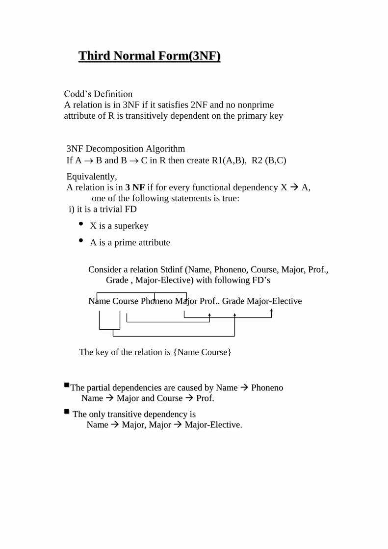
CCoonnssiiddeerr aa rreellaattiioonn SSttddiinnff ((NNaammee,, PPhhoonneennoo,, CCoouurrssee,, MMaajjoorr,, PPrrooff..,,

GGrraaddee ,, MMaajjoorr--EElleeccttiivvee)) wwiitthh ffoolllloowwiinngg FFDD’’ss

NNaammee CCoouurrssee PPhhoonneennoo MMaajjoorr PPrrooff.... GGrraaddee MMaajjoorr--EElleeccttiivvee

TThhee ppaarrttiiaall ddeeppeennddeenncciieess aarree ccaauusseedd bbyy NNaammee PPhhoonneennoo

NNaammee MMaajjoorr aanndd CCoouurrssee PPrrooff..

TThhee oonnllyy ttrraannssiittiivvee ddeeppeennddeennccyy iiss

NNaammee MMaajjoorr,, MMaajjoorr MMaajjoorr--EElleeccttiivvee..

The key of the relation is {Name Course}

2NF Decomposition: R1(Name, Phoneno, Major, Major-Elective)

R2(Course,Prof.)

R3(Name,Course,Grade)

3NF Decomposition: R1-1(Name,Phoneno,Major)

R1-2(Major, Major-Elective)

R2(Course, Prof.)

R3(Name,Course,Grade)

BCNF

CCoonnssiiddeerr aa rreellaattiioonn SSttddiinnff ((NNaammee,, PPhhoonneennoo,, CCoouurrssee,, MMaajjoorr,, PPrrooff..,,

GGrraaddee ,, MMaajjoorr--EElleeccttiivvee)) wwiitthh ffoolllloowwiinngg FFDD’’ss

NNaammee CCoouurrssee PPhhoonneennoo MMaajjoorr PPrrooff.... GGrraaddee MMaajjoorr--EElleeccttiivvee

TThhee ppaarrttiiaall ddeeppeennddeenncciieess aarree ccaauusseedd bbyy NNaammee PPhhoonneennoo

NNaammee MMaajjoorr aanndd CCoouurrssee PPrrooff..

TThhee oonnllyy ttrraannssiittiivvee ddeeppeennddeennccyy iiss

NNaammee MMaajjoorr,, MMaajjoorr MMaajjoorr--EElleeccttiivvee..

The key of the relation is {Name Course}

Need For BCNF arises when X A and A B where B is a subset

of X

Student (Name, Course, Teacher) and

Name Course

Teacher

Name Course Teacher

A C1 T1

B C1 T1

C C2 T2

Note: Name, Course

is the primary key of

Student

A relation is in BCNF if whenever a functional dependency

X A holds then, either

i) X is a super key of R, or

ii) X A is trivial (A is subset of X)

LLoosssslleessss BBCCNNFF DDeeccoommppoossiittiioonn

FFoorr RR((AA,,BB,,CC)) iiff AA,,BB CC aanndd CCBB,, decompose R into R1(C,B) and

R2 (R - B) NNoottee:: DDeeppeennddeennccyy NNoonn--pprreesseerrvviinngg

Difference with 3NF: A cannot be a prime attribute

A relation R is in BCNF if it is in 1NF and for every collection C of

fields, if any field not in C is functionally dependent on C, then C

R

Answer 4

a) A transaction is a unit of program execution that accesses and possibly updates

various data items.

A transaction must see a consistent database.

During transaction execution the database may be inconsistent.

When the transaction is committed, the database must be consistent.

Two main issues to deal with:

Failures of various kinds, such as hardware failures and system crashes

Concurrent execution of multiple transactions

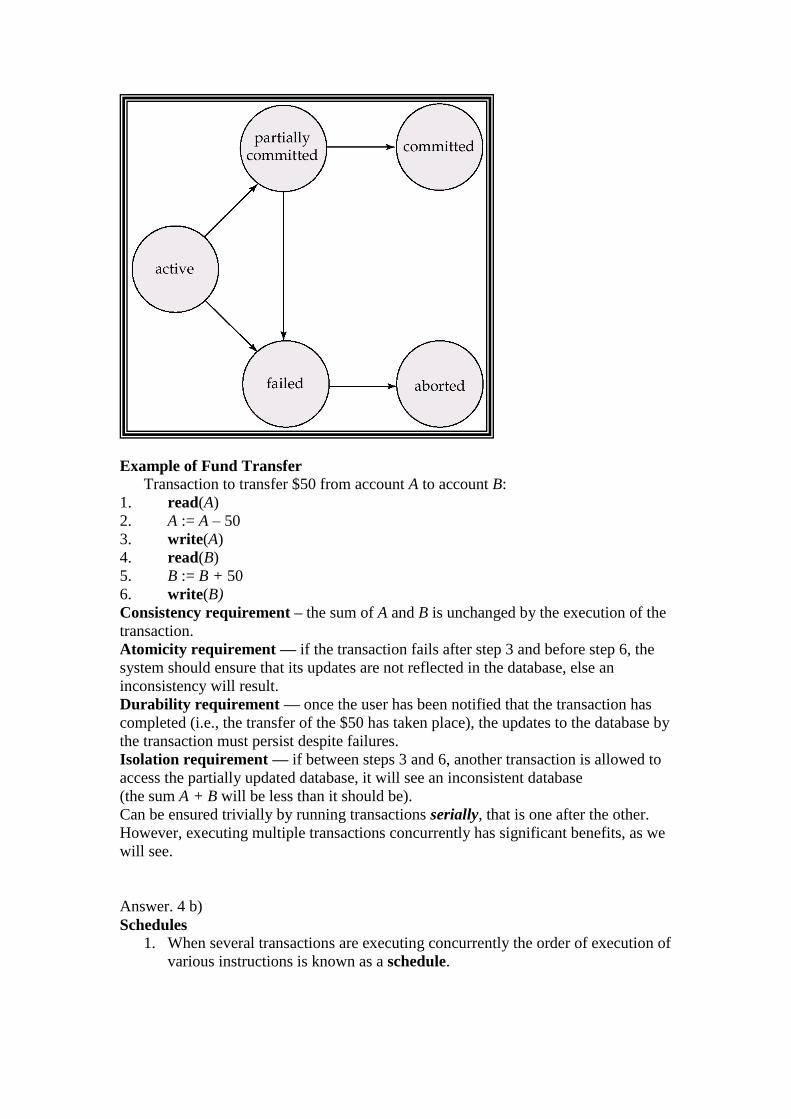
Transaction State

1. Active, the initial state; the transaction stays in this state while it is executing

2. Partially committed, after the final statement has been executed.

3. Failed, after the discovery that normal execution can no longer proceed.

4. Aborted, after the transaction has been rolled back and the database restored

to its state prior to the start of the transaction. Two options after it has been

aborted:

a. restart the transaction – only if no internal logical error

b. kill the transaction

5. Committed, after successful completion.

Example of Fund Transfer

Transaction to transfer $50 from account A to account B:

1. read(A)

2. A := A – 50

3. write(A)

4. read(B)

5. B := B + 50

6. write(B)

Consistency requirement – the sum of A and B is unchanged by the execution of the

transaction.

Atomicity requirement — if the transaction fails after step 3 and before step 6, the

system should ensure that its updates are not reflected in the database, else an

inconsistency will result.

Durability requirement — once the user has been notified that the transaction has

completed (i.e., the transfer of the $50 has taken place), the updates to the database by

the transaction must persist despite failures.

Isolation requirement — if between steps 3 and 6, another transaction is allowed to

access the partially updated database, it will see an inconsistent database

(the sum A + B will be less than it should be).

Can be ensured trivially by running transactions serially, that is one after the other.

However, executing multiple transactions concurrently has significant benefits, as we

will see.

Answer. 4 b)

Schedules

1. When several transactions are executing concurrently the order of execution of

various instructions is known as a schedule.

2. The concept of serializability of schedules is used to identify which schedules

are connect when transaction executions have interleaving of their operations

in the schedules.

3. Types of schdeules

a. Serial schedules

b. Non-serial schedules

c. Conflict schedules

d. View schedules

Serial schedules

1. Two schedules T1 and T2 are called serial schedule if the operations of each

transaction are executed consecutively, without any interleaved operations

from the other transaction.

2. In a serial schedule, entire transaction are performed in serial order T1 and

then T2 OR T2 then T1.

Non-serial Schedule

Two schedules T1 and T2 are called non-serial schedule if the operations of each

transaction are executed non-consecutively with interleaved operations from the

other transaction.

Conflict schedule

The precedence graph contains no cycle is called conflict serializable schedule

View Schedule

1. The precedence graph contains a cycle is called view schedule.

2. If the graph contains no cycle, then the schedule S is conflict serializable.

3. If the graph for S has a cycle, then schedule S is not conflict serializable.

Conflict Serializability

Instructions li and lj of transactions Ti and Tj respectively, conflict if and only if

there exists some item Q accessed by both li and lj, and at least one of these

instructions wrote Q.

1. li = read(Q), lj = read(Q). li and lj don’t conflict.

2. li = read(Q), lj = write(Q). They conflict.

3. li = write(Q), lj = read(Q). They conflict

4. li = write(Q), lj = write(Q). They conflict

Intuitively, a conflict between li and lj forces a (logical) temporal order between

them. If li and lj are consecutive in a schedule and they do not conflict, their

results would remain the same even if they had been interchanged in the schedule.

View Serializability

Let S and S´ be two schedules with the same set of transactions. S and S´ are view

equivalent if the following three conditions are met:

1. For each data item Q, if transaction Ti reads the initial value of Q in

schedule S, then transaction Ti must, in schedule S´, also read the initial value

of Q.

2. For each data item Q if transaction Ti executes read(Q) in schedule S,

and that value was produced by transaction Tj (if any), then transaction Ti

must in schedule S´ also read the value of Q that was produced by transaction

Tj .

3. For each data item Q, the transaction (if any) that performs the final

write(Q) operation in schedule S must perform the final write(Q) operation in

schedule S´.

As can be seen, view equivalence is also based purely on reads and writes

alone.

Recoverability

Need to address the effect of transaction failures on concurrently running transactions.

1. Recoverable schedule — if a transaction Tj reads a data items previously

written by a transaction Ti , the commit operation of Ti appears before the

commit operation of Tj.

2. The following schedule (Schedule 11) is not recoverable if T9 commits

immediately after the read

Schedule 11

3. If T8 should abort, T9 would have read (and possibly shown to the user) an

inconsistent database state. Hence database must ensure that schedules are

recoverable.

Cascading rollback – a single transaction failure leads to a series of transaction

rollbacks. Consider the following schedule where none of the transactions has yet

committed (so the schedule is recoverable)

Schedule 12

If T10 fails, T11 and T12 must also be rolled back.

Can lead to the undoing of a significant amount of work

Cascadeless schedules — cascading rollbacks cannot occur; for each pair of

transactions Ti and Tj such that Tj reads a data item previously written by Ti, the

commit operation of Ti appears before the read operation of Tj.

Every cascadeless schedule is also recoverable

It is desirable to restrict the schedules to those that are cascadeless

Answer 4 C)

Distributed Database:

A distributed database system consists of loosely coupled sites that share no

physical component

Database systems that run on each site are independent of each other

Transactions may access data at one or more sites

Data Replication

A relation or fragment of a relation is replicated if it is stored redundantly in two

or more sites.

Full replication of a relation is the case where the relation is stored at all sites.

Fully redundant databases are those in which every site contains a copy of the

entire database.

Advantages of Replication

Availability: failure of site containing relation r does not result in

unavailability of r is replicas exist.

Parallelism: queries on r may be processed by several nodes in

parallel.

Reduced data transfer: relation r is available locally at each site

containing a replica of r.

Disadvantages of Replication

Increased cost of updates: each replica of relation r must be updated.

Increased complexity of concurrency control: concurrent updates to

distinct replicas may lead to inconsistent data unless special

concurrency control mechanisms are implemented.

One solution: choose one copy as primary copy and apply

concurrency control operations on primary copy

Data Fragmentation

Division of relation r into fragments r1, r2, …, rn which contain sufficient

information to reconstruct relation r.

Horizontal fragmentation: each tuple of r is assigned to one or more

fragments

Vertical fragmentation: the schema for relation r is split into several smaller

schemas

o All schemas must contain a common candidate key (or superkey) to

ensure lossless join property.

o A special attribute, the tuple-id attribute may be added to each schema

to serve as a candidate key.

Example : relation account with following schema

Account = (account_number, branch_name , balance )

Advantages of Fragmentation

Horizontal:

o allows parallel processing on fragments of a relation

o allows a relation to be split so that tuples are located where they are

most frequently accessed

Vertical:

o allows tuples to be split so that each part of the tuple is stored where it

is most frequently accessed

o tuple-id attribute allows efficient joining of vertical fragments

Vertical and horizontal fragmentation can be mixed.

o Fragments may be successively fragmented to an arbitrary depth.

Replication and fragmentation can be combined

o Relation is partitioned into several fragments: system maintains several

identical replicas of each such fragment.

Answer. 5 a)

Lock: A mechanism to control concurrent access to a data item by competing

transactions.

Locking protocol: A set of rules followed by all transactions while requesting and

releasing locks.

Types of Lock

Granularity of locks:

Can be at the field level, record level, or disk block level, or table level.

Less granular locks provides better concurrency, but increases locking

overhead since more lock/unlock operations are needed.

Types of locks:

Read lock or shared lock (lock-S): Data item can be read but not

updated by the locking and other transactions.

Write lock or exclusive lock (lock-X): Data items can be read and

updated by the locking transaction, but not by other transactions.

Concurrency control manager can upgrade read locks to write locks, or

downgrade write locks to read locks, as requested.

All locking operations (read_lock, write_lock) precede the first unlock operation in

the transactions. Two phases:

• expanding phase: new locks on items can be acquired but

none can be released

• shrinking phase: existing locks can be released but no new

ones can be acquired

Graph Based Protocol

1. To acquire a prior knowledge, we impose a partial ordering on the set

D={d1,d2,…..dn} of all data item. If didj, then any transaction accessing

both di and dj must access di before accessing dj.

2. The partial ordering implies that the set D may now be viewed as a directed

acyclic graph called a database graph.

3. For the sake the simplicity, we will restrict our attention to only those graphs

that are rooted trees.

4. Tree protocol is restricted to employ only exclusive locks.

5. In the tree protocol, the only lock instruction allowed is lock-X. Each

transaction Ti can lock a data item at ,most once, and must observe the

following rules:

a. The first lock by Ti may be any data item.

b. Subsequently, a data item Q can be locked by Ti only if the parent of Q

is currently locked by Ti.

c. Data items may be unlocked at any item.

d. A data item that has been locked and unlocked by Ti cannot

subsequently be relocked by Ti.

Graph-based protocol Advantages & Disadvantages over two-phase locking

Advantages

It is deadlock-free so no rollbacks are required.

Unlocking may occur earlier. Earlier unlocking may lead to shorter

waiting times, and to an increase in concurrency.

Disadvantages

Transaction may have to lock data items that it does not access.

Answer 5 b)

Deadlock: when each of two transactions is waiting for the other to release an

item.

Approaches for solution:

read_lock(Y); read_lock(X);

read_item(Y);

unlock(Y); read_item(X);

X:=X+Y; write_lock(X); write_item(X);

unlock(X);

read_lock(X);

read_item(X);

write_lock(Y);

unlock(X); read_item(Y);

Y:=X+Y; write_item(Y); unlock(Y);

not two-phase locking two-phase locking

o deadlock prevention protocol: every transaction must lock all items it

needs in advance

o deadlock detection (if the transaction load is light or

transactions are short and lock only a few items):

Livelock: a transaction cannot proceed for an indefinite period of time while

other transactions in the system continue normally.

o Solution: fair waiting schemes (i.e. first-come-first-served)

There are two principal methods for dealing with deadlock problems:

– Deadlock prevention protocol

– Deadlock detection and recovery process

Deadlock prevention protocol

This protocol ensures the system will ensure that the system will not go into

deadlock state. There are different methods can be used for deadlock prevention:

– The simplest scheme requires that each transaction locks all its data

item before it starts execution.

– Another method for prevention of deadlock is to impose a partial

ordering of all data items and require that a transaction can lock a data

item only in the order specified by partial order.

– Another approach for the prevention of deadlock is to use pre-emption

and transaction rollbacks.

Deadlock Detection and Recovery

If a system does not imply some protocol that ensures deadlock freedom, then a

detection and recovery scheme must be used.

Deadlock Detection

Deadlock can be described previously in terms of a directed graph called a

wait a graph.

This graph consist of a pair G=(V,E) where V is a set of vertices and E is set

of edges.

Each element in the set E of edges is an ordered pair Ti Tj.

If TiTj is in E, then there is a directed edge from transaction Ti+Tj,

implying that transaction Ti, is waiting for ransaction Tj to releases a data item

that it needs.

A deadlock exist in the system if and only if the wait for graph contains a

cycle. Each transaction involved in the cycle is said to be deadlocked.

Deadlock Recovery

When a detection algorithm determines that a deadlock exists, the system must

recover from deadlock.

The most common solution is to rollback one or more transactions to break the

deadlock. There actions need to be taken:

1. Selection of a victim

2. Rollback

3. Starvation

As Tanenbaum shows, when the wait-for graph is computed at a central

location that collects messages from the various systems involved in

transactions, it is easy to find also false, or spurious, or phantom deadlocks

as in the following picture

when Q first releases S and then P requests S, but the messages delivered to

the coordinator that collects the messages arrive in the wrong order. Then

the coordinator believes that a deadlock has arisen and kills unnecessarily P

or Q. Of course, if Q was following a 2-phase locking policy, it would not

release any lock until it had acquired every lock it needed. Thus phantom

deadlocks would not arise if 2-phase locking is followed.

Answer 5 c) i) Time stamping protocol for concurrrency control

Time stamping ids a concurrency protocol in which the fundamental goal is to

order transactions globally in such a way that older transactions get priority in

the event of a conflict.

In this method, if a transaction attempts to read or write a data item, then a

read or write operation is allowed only if the last updated on that data item

was carried out by an older transaction.

Otherwise the transaction, requesting the read or write is restarted and given a

new timestamp. The restarted transaction is assigned a new timestamp to

prevent it from continuously aborting and restarting.

In this method, sequence of transaction is selected in advance by using time

stamping concept.

We associate a unique, fixed non-decreasing numbers called the timestamp to

each transaction in the system. This number can be the system clock value, i.e.

when the transaction enters the system the current value of the clock is

assigned to that transaction as the timestamp value.

We can also use a logical number that is incremented after a new transaction

enters the system.

A transaction with a smaller timestamp value is considered to be an adder

transaction than another transaction with a larger time stamp value.

In other words, if a transaction T1 has been assigned a timestamp S1 and a

new transaction T2 enters the system with a time stamp value S2 then S1<S2

and system will allow the transaction T1 to run first followed by the

transaction T2.

If any conflict is found between transaction using timestamp based system,

one of the conflicting transaction is rolled back.

There are two types of timestamps:

W-time stamp (Q): Denotes the largest time stamp of any transaction that

executed write(Q) successfully.

R-Time stamp (Q): Denotes the largest time stamp of any transaction that

executed read(Q) successfully.

ii) Checkpoints

Storage Structure

Volatile storage:

– does not survive system crashes

– examples: main memory, cache memory

Loss of Volatile Storage- It can be recovered using various methods. e.g., Log-

based recovery, Buffer Management, checkpoints, and shadow paging techniques.

Checkpoints or syncpoints or save points

A checkpoint is a point of synchronization b/w the database and the

transaction log file.

All buffers are force-written to secondary storage at the checkpoint.

Checkpoints are schedules at predetermined interval and involves operations

like writing all log records in main memory to secondary storage.

If the transactions are executed serially, when a failures occurs, we check the

log file to find the transaction that started before the last chcekpoint.