A global search framework for practical three-dimensionalpacking with variable carton orientations

Author

He, Yaohua, Wu, Yong, de Souza, Robert

Published

2012

Journal Title

Computers & Operations Research

DOI

https://doi.org/10.1016/j.cor.2011.12.007

Copyright Statement

© 2011 Elsevier. This is the author-manuscript version of this paper. Reproduced in accordancewith the copyright policy of the publisher. Please refer to the journal's website for access to thedefinitive, published version.

Downloaded from

http://hdl.handle.net/10072/44199

Griffith Research Online

https://research-repository.griffith.edu.au

1

A Global Search Framework for Practical

Three-Dimensional Packing with Variable Carton Orientations

Yaohua He a, c*, Yong Wu

b, Robert de Souza

c

a Dept. of Industrial and Systems Engineering / Office of the Provost (PVO), National University of Singapore, Singapore 117576

b Department of International Business and Asian Studies, Gold Coast Campus, Griffith University, QLD 4222 Australia

c The Logistics Institute - Asia Pacific, National University of Singapore, Singapore 119613

Abstract

This article aims to tackle a practical three-dimensional packing problem, where a number of cartons

of diverse sizes are to be packed into a bin with fixed length and width but open height. Each carton is

allowed to be packed in any one of the six orientations, and the carton edges are parallel to the bin edges.

The allowance of variable carton orientations exponentially increases the solution space and makes the

problem very challenging to solve. This study first elaborately devises the packing procedure which converts

an arbitrary sequence of cartons into a compact packing solution and subsequently develops an improved

genetic algorithm (IGA) to evolve a set of solutions. Moreover, a novel global search framework (GSF),

utilizing the concept of evolutionary gradient, is proposed to further improve the solution quality. Numerical

experiments indicate that IGA provides faster and better results and GSF demonstrates its superior

performance, especially in solving relative large-size and heterogeneous instances. Applying the proposed

algorithms to some benchmarking cases of the three-dimensional strip packing problem also indicates that

the algorithms are robust and effective compared to existing methods in the literature.

Keywords: packing; loading; three-dimensional; genetic algorithm; global search; evolutionary gradient

1. Introduction

Bin packing, or container/pallet loading, is a very common but important task in the manufacturing and

logistics industries. However, even after the problem has been researched for several decades, many of

packing tasks are still accomplished manually, i.e., the workers stow bins or containers according to their

experience and judgement. It is evident from operational observations and the literature that manual packing

may not optimally utilize the valuable bin/container space, and the volume utilization can be significantly

improved with the support of computer-generated solutions. Exact algorithms, due to the complexity and

combinatorial explosive nature, can only solve small-size problems to optimality with the current computing

technology. For most practical applications, heuristics and meta-heuristics are still the best choices to

achieve optimal or near-optimal solutions within reasonable time.

This study solves a practical three-dimensional packing problem by using heuristics and meta-heuristics

with the purpose of obtaining high quality solutions as fast as possible. In the investigated problem, a number

* Corresponding Author: Tel: +65-90438961, Fax: +65-67771434

E-mail: Yaohua.He001@gmail.com (Y. He), yong.wu@griffith.edu.au, wuyong@pmail.ntu.edu.sg (Y. Wu)

2

of cartons of diverse sizes are to be stowed into a paperboard bin with fixed length and width but open height

(subject to physical limit), i.e., the bin height can be trimmed to fit the content of the bin to save transport

cost (e.g., when air transportation is used). Each carton is allowed to be packed in any one of the six

orientations, and the carton edges are parallel to the bin edges (we will call this as variable orientations

hereafter). The cartons need not be stowed in layers or walls, and no so-called guillotine constraint is

imposed to the packing process.

According to the typology of cutting and packing problems introduced by Wäscher et al. (2007), our

investigated problem is a three-dimensional packing problem with one variable dimension, different from the

traditional three-dimensional bin packing problem (3D-BPP) where a selected subset of a number of cartons

are packed into a bin with fixed length, width and height to maximize the volume utilization, or where a

large number of cartons are packed into identical bins with the objective to minimize the number of bins

used. For this problem, the variable bin height poses a greater challenge in providing high-quality solutions

since usually no selection of cartons is allowed, i.e., all cartons need to be packed, and when the bin is not

fully packed the extra height will be trimmed. The flexibility of carton orientations further expands the

solution space significantly and thus increases the difficulty in finding the optimal solutions. Up to now, such

a problem with both variable bin height and variable carton orientations has only been studied by a few

researchers.

It should be noted that the problem under investigation possesses some characteristics of the

three-dimensional strip packing problem (3D-SPP). However, compare with the traditional 3D-SPP in the

literature, it presents two important features: a) the physical bin height (which corresponds to strip length in

3D-SPP) limit is relatively short due to the fact that paperboard bins are used, which limits the maximum

loading height/weight; whereas in 3D-SPP the strip length is usually much longer than both the strip width

and the strip height, thus the term ‘strip’ is used; b) the cartons that are to be packed are ‘generated’ on the

fly in various dimensions, which presents a very heterogeneous packing problem; in contrast in traditional

3D-SPP it is common to see boxes (in small bunches) have the same dimensions. The demand to pack highly

heterogeneous cartons in a relatively small paperboard bin makes layer-building heuristics unsuitable (e.g., in

extreme case, every carton to be packed may belong to a different carton type, this may make layer-building

almost impossible). Although the current problem represents a special case of 3D-SPP, the concept of ‘bin’

will still be used for ease of description in this paper for two reasons: a) paperboard bins are used in practical

packing; and b) there is no significant difference between the maximum (variable) bin height and the fixed

bin length and fixed bin width.

The solution techniques for packing problems can be classified into three types:

Exact methods based on mathematical programming belong to the first type. Chen et al. (1995)

provided a mixed integer linear programming (MILP) model to solve the 3D-BPP with variable orientations.

Due to the strong NP-hardness of the problem, this MILP model only solved a small instance with 6 cartons

to optimality. Martello et al. (2000) and den Boef et al. (2005) presented an exact algorithm for loading a

single bin and discussed the lower bounds for the 3D-BPP. Martello et al. (2007) presented an algorithm to

3

solve moderate instances to optimality for the general 3D-BPP and its robot-packable variant. Fekete et al.

(2007) developed a two-level tree search algorithm for solving higher-dimensional packing problems to

optimality, but their computational results reported were on the optimal solutions for two-dimensional test

problems from the literature. Ceselli and Righini (2008) presented a branch-and-price algorithm for the exact

optimization of the ordered open-end bin-packing problem defined by Yang and Leung (2003), where the

items to be packed are sorted in a given order and the capacity of each bin can be exceeded by the last item

packed into the bin.

Heuristics and approximate algorithms comprise the second type. Lim et al. (2005) conducted a

comprehensive review on the heuristics studied by many researchers, from which it could be seen that most

heuristics were on the wall- or layer-building of the traditional 3D-BPP to pack a selected subset of a number

of cartons into a bin/container pursuing high volume utilization. For example, George and Robinson (1980)

presented a wall-building approach heuristic without restrictions on the carton orientations for identical

containers. Bischoff and Marroitt (1990) evaluated 14 different heuristics based on the George-Robinson

framework. Bischoff et al. (1995) proposed a pallet loading heuristic for non-identical cartons where the

stability of the pallet was considered. Pisinger (2002) offered a heuristic based on the wall-building approach,

where strips and layers were created so that the 3D-BPP could be decomposed into smaller sub-problems.

Baltacioglu et al. (2006) developed a new heuristic algorithm using rules to mimic human intelligence to

solve the 3D-BPP. Faroe et al. (2003) provided a heuristic for packing cartons into a minimum number of

identical containers based on guided local search, however, no variable orientation was allowed. Huang and

He (2009) developed a heuristic algorithm for the traditional 3D-BPP without orientation constraints based

on the concept of caving degree inspired by an old adage “Gold corner, silver side and grass belly” from

Chinese Weiqi (a board game), which achieved very high volume utilization for the benchmark instances

provided by Bischoff and Ratcliff (1995) and later solved by so many researchers, such as Lim et al. (2005),

Bortfeldt and Gehring (1998, 2001) and Zhang et al. (2007).

The third choice is meta-heuristics, such as genetic algorithms, tabu search and simulated annealing, are

widely used. Gehring and his colleagues have published a number of papers on meta-heuristic methods for

3D-BPP. Gehring and Bortfeldt (1997) first presented a genetic algorithm and then (2002) provided a

parallel genetic algorithm for single container loading with stronger heterogeneous cartons. Bortfeldt and

Gehring (1998) first applied tabu search and then (2001) presented a hybrid genetic algorithm for single

container loading, finding that the former was suitable to weakly heterogeneous cases but the latter suitable

to strongly heterogeneous cases. Lodi et al. (2002) provided a tabu search framework by exploiting a

constructive heuristic to evaluate the neighborhood where the carton orientations were fixed. Zhang et al.

(2007) proposed a simulated annealing algorithm combined with a bin-loading heuristic to solve the classic

3D-BPP. Crainic et al. (2008a) introduced a two-level tabu search where the first level aimed to reduce the

number of bins and the second optimized the bin packing of cartons with fixed orientations. Egeblad and

Pisinger (2009) examined 2D/3D knapsack packing problems using simulated annealing. Goncalvez and

Resende (2012) proposed a parallel random-key-based genetic algorithm using layer-building heuristics.

4

Another classification for 3D loading problems by Fanslau and Bortfeldt (2010) divides packing

algorithms into exact and heuristic methods. The latter can be further divided into three groups: conventional

heuristics, meta-heuristics and tree search methods. Bortfeldt and Mack (2007) presented a layer-building

heuristic method for the 3D-SPP, where tree search algorithms were adopted to determine the best layer

depths and to obtain the best strip directions and strip dimensions for a given layer. Their method did not

involve any supplementary loading restrictions, particularly no supporting constraints are imposed.

Regarding the heuristic packing approaches (Pisinger, 2002), wall building, stack building, horizontal layer

building, block building and guillotine cutting were often used.

Allen et al. (2011) proposed a hybrid placement strategy for the 3D-SPP, which is actually a

decomposition method: one bigger sub-set of items are packed via three-dimensional best fit heuristic, the

other smaller sub-set of items are packed through a tabu search algorithm, thus saving the search time.

Through analyzing the existing solution methods, the following observations can be made: (1) Most of

heuristics are based on the wall-building with some modifications, which are in nature greedy techniques that

might stuck at local optimal solutions and away from the global optimality; (2) Exact methods are based on

mathematical programming and graph theory by reducing the original problem to a theoretically solvable

model, which at the moment would be virtually impossible to guarantee the global optimality for practical

3D problems, especially for those with variable orientations; (3) Meta-heuristics are the present best choice,

which can search much larger feasible space than the simple heuristics and converge much faster than the

exact methods, hence make it realistic to obtain optimal or near-optimal solutions within reasonable search

time.

However, in practical applications of the meta-heuristics, the users usually have to tune the algorithm

parameters according to the problem conditions and carry out a number of tests to select the best solution as

the real stowage plan. In general, the users hope to have lower variance of solutions in the tests, which may

imply the algorithm has higher search performance and convergence. But the search ability of an algorithm

depends on the prevailing problem conditions. As long as the solution variance exists, all the better solutions

via the algorithm are still possible. So how to fully utilize the search ability until the average deviation of

solutions turns to be null will be considered in this paper.

This paper further studies the problem proposed in Wu et al. (2010) in which an exact mathematical

model based on Chen et al. (1995) was first developed and a genetic algorithm was subsequently designed

and implemented with a heuristic packing procedure (or decoding routine). In this paper, we first improve

the decoding procedure aiming at tighter packing and higher computational efficiency; and then redesign and

implement a genetic algorithm with well tailored components based on the work of He (2007 and 2009).

Further, we propose a global search framework based on the concept of evolutionary gradient (He and Hui,

2009 and 2010) and devise several scenarios of the framework for simulation experiments. A suitable

scenario is selected for the practical 3D packing problem through numerical experiments.

2. Problem Description

5

The investigated problem originates from a real-world application, for which Wu et al. (2010) provided

an MILP model and a basic GA. The packing objective is to minimize the height H of the paperboard bin

used when packing N cartons so that logistics costs can be saved since the packed bins are transported via air.

As mentioned earlier, the height of bins is subject to physical limit.

2.1 Bins and Cartons

In the practical problem, a rectangular bin with fixed length and width (L×W) is available to pack a

number (N) of rectangular cartons for shipping (see Fig. 1a). The height (H) of the bin can be trimmed to fit

the cartons packed, but cannot exceed the physical limit height, Hmax.

Each carton i has a fixed size of li×wi×hi (centimeter), where li, wi and hi are the length, width and

height of carton i. Without loss of generality, we assume li ≥wi ≥hi (see Fig. 1b). Each carton may be packed

into the bin in any one of the six orientations that keep the carton edges parallel to the bin edges. The cartons

need not be stowed in layers or walls, and no so-called guillotine constraint is imposed to the packing

process.

2.2 Reference Points, Cage Bin and Orientations

The Cartesian coordinate system is used to locate a carton in the bin (see Fig. 1a). Martello et al. (2000)

proposed corner points as candidate locations where a carton could be placed, which needs be calculated by

using a 2D algorithm and bears the shortcoming that some space of the bin is not covered and thus cannot be

exploited. Zhang et al. (2007) presented possible placement points for a carton to be placed, a selected point

of which is just a possible location for a carton, but may not be the final position because of the later parallel

moves for compact packing. Therefore placement points belong to a kind of reference points. Crainic et al.

(2008b) introduced extreme points and corresponding heuristics for 3D-BPP without any further parallel

moving, even though extreme points are generated in the same way as placement points. We adopt the

concept of reference points in this work.

When each carton i is packed into the bin, the carton edges are parallel to the bin edges, as shown in Fig.

1(b). A reference point in the bin is denoted by its coordinates (x, y, z). An empty bin has only one reference

point (0, 0, 0), and every time when the left-front-bottom corner of carton i with li×wi×hi is assigned at (xi, yi,

zi), three new reference points will be generated depending on the carton orientation, such as (xi+li, yi, zi), (xi,

Fig. 1 A bin, a carton and a cage bin

x

y

z

L

H

W

(a) A bin with L×W×H

x

y

z

li

hi

wi

front

bottom

left

(b) A carton i with li×wi×hi

x

y

z

lc

hc

wc

(c) A cage bin with lc×wc×hc

6

yi+wi, zi) and (xi, yi, zi+hi).

The concept of cage bin is utilized in our work. A cage bin is a virtual bin and is defined as the smallest

rectangular box (with dimensions of lc×wc×hc) that is able to encase all the cartons already packed in the bin;

therefore, the cage bin changes as the packing of cartons proceeds. For example, Fig. 1c shows the cage bin

encasing two cartons packed so far in the bin.

Each carton can be placed into the bin in any one of its six orientations. That is to say, although the

original size (li×wi×hi) of carton i is fixed, its orientation in the bin is not pre-fixed. To make the total packing

compact, each carton i can take any one of its six orientations as depicted in Fig. 2, where γi denote the

orientation number, γi∈{1, 2, 3, …, 6}, i =1, 2, 3, …, N.

2.3 An MILP Solvable Example

Mathematically proven global optimal solutions, no matter how difficult to derive, are always desirable

for first of all, providing a benchmark for other methods; and secondly, applying to the actual problem when

the solutions are relatively easy to achieve. Wu et al. (2010) adopted the MILP model presented in Chen et al.

(1995) and coded in GAMS. Though computing resources have advanced significantly in the past two

decades, the mathematical approach still seems to be less practical, as shown by the following example.

Table 1 presents the original sizes of a set of cartons to be packed into a small bin with fixed length and

width L×W = 80×58 cm, the Hmax= 95 cm. This example (called SM00) will be used to illustrate the proposed

solution techniques in this paper.

Table 1. The sizes of the cartons in SM00

Carton i li×wi×hi Carton i li×wi×hi

1 36×36×36 6 40×31×21

2 59×39×20 7 31×31×17

3 54×40×21 8 31×17×16

4 58×37×21 9 26×23×14

5 52×33×20 10 33×21×4

The above example was solved by the commercial solver CPLEX 11.2 based on the GAMS model in

Wu et al. (2010). CPLEX 11.2 finds the solution with the height 68 cm after 1006 seconds, and proves the

optimality at 1144 second. Fig. 3 shows the packing configuration of the optimal solution.

It can be observed from the example that mathematical approach still takes a long time to solve a

relatively small practical instance. An optimistic estimation of the maximum number of cartons the

mathematical model can handle under current computational resources would be below 20, or even 15. In

li

hi

wi

γi = 1 li

wi

hi

γi = 2

hi

wi li

γi = 3

hi wi

li

γi = 4 hi

wi

li

γi = 5

li

hi wi

γi = 6

Fig. 2 Six orientations of carton i

Fig. 3 Optimal packing for SM00

7

Wu et al. (2010), such a maximum number was 12 for CPLEX 11.0 with 2 hours’ running time and in a

number of cases where less than 12 cartons were presented, CPLEX 11.0 failed to find the proven optimal

solutions within the specified running time. Therefore, to provide solutions for practical problems within

reasonable time, alternative approaches must be used.

3. The GA Coding and Decoding Procedures

To solve a problem by GA, the first task is to represent a solution of the problem as a chromosome, P.

This representation is called coding. For combinatorial optimization, there are several representation

methods, among which permutation-based representation (Gen and Cheng, 1997) and random-key (Bean,

1994) are often used. The procedure to change a chromosome P into a phenotype solution with an objective

value f(P) is called decoding.

3.1 Coding of an Arbitrary Solution

A mixed chromosome, which includes both the carton packing order and the carton orientations, is

adopted to represent a packing solution in this research. The mixed chromosome P = (P1, P2) consists of two

parts: P1=(π1, π2, π3, …, πN) is a carton sequence, πi∈{1, 2, 3, …, N}, i =1, 2, 3, …, N; P2 = (γ1, γ2, γ3, …, γN)

is an orientation sequence, γi∈{1, 2, 3, …, 6}, i =1, 2, 3, …, N. Fig. 4 shows a sample chromosome for a

problem with 10 cartons, where each carton πi in P1 is given a corresponding orientation γi in P2.

3.2 Decoding Procedure

The decoding routine converts a chromosome into a feasible packing solution. Cartons in the given

chromosome are processed sequentially, and their coordinates and relative positions are determined at the

same time.

3.2.1 Carton List and Reference Point List

To decode a chromosome, two data lists, a carton list (c-list) and a reference point list (ref-point-list),

are used to store the relevant data. A c-list corresponds to a chromosome. Each element i in the c-list contains

the following information: carton no. πi, orientation no. γi, original size (li×wi×hi), orientational dimensions

(lni×wni×hni) (derived from orientation no. γi and original size), coordinates (xi, yi, zi) (to be determined), and

relative positions (left-carton-no, front-carton-no, bottom-carton-no) (to be determined). Table 2 shows a

sample c-list for the sample chromosome in Fig. 4. The coordinates and relative positions of the cartons are

variables to be determined so that all cartons do not intersect with each other while maintaining a packing

solution as compact as possible. When the coordinates and relative positions of the cartons in the c-list are

determined through the decoding procedure (i.e. the packing procedure), the c-list is changed into a packing

solution.

Fig. 4 A sample mixed chromosome

1 10 6 8 3 5 2 9 7 4 1 1 4 4 5 3 6 4 5 1

Carton sequence P1 Orientation sequence P2

8

Table 2. The sample carton list for the sample chromosome in Fig. 4

Original size New dimensions Coordinates Relative positions

i ππππi γi li wi hi lni wni hni xi yi zi left front bottom

1 1 1 36 36 36 36 36 36

2 10 1 33 21 4 33 21 4

3 6 4 40 31 21 31 21 40

4 8 4 31 17 16 17 16 31

5 3 5 54 40 21 21 54 40

6 5 3 52 33 20 33 52 20

7 2 6 59 39 20 20 39 59

8 9 4 26 23 14 23 14 26

9 7 5 31 31 17 17 31 31

10 4 1 58 37 21 58 37 21

Based on the concept of reference points in §2.2, a ref-point-list is adopted to store the information of

the ref-points generated in the process of packing: coordinates, the type of the point, the temporary indices,

occupied status. As stated earlier, an empty bin has one ref-point (0, 0, 0), and the first carton is assigned to

this point hence marked as “occupied”. And then every time when carton πi with lni×wni×hni is assigned at

(xi, yi, zi), three new reference points, (xi+lni, yi, zi), (xi, yi+wni, zi) and (xi, yi, zi+hni), are generated and added

to the ref-point-list as “not occupied yet”. A feasible ref-point for the current carton to be packed is the one

which ensures that the carton will not intersect with any cartons packed so far or the bin itself. If a ref-point

is selected to assign a carton, this point may not be the final position of the carton because of the later

parallel moves (introduced in §3.2.2), which try to move the carton along the x-, y- and z-axis to make the

packing more compact.

To efficiently conduct the parallel moving, we classify the ref-points into three types: type 1, (xi+lni, yi,

zi); type 2, (xi, yi+wni, zi); and type 3, (xi, yi, zi+hni). Furthermore, the just packed carton πi is recorded as the

adjacent carton of these three points, (xi+lni, yi, zi), (xi, yi+wni, zi) and (xi, yi, zi+hni), which is convenient to

determine the relative positions of the packed cartons. Therefore, each ref-point k in the ref-point list should

include the following information: coordinates (xk, yk, zk), the adjacent carton to this point (adj_carton), type

no. (type 1, 2 or 3), two indices index1 and index2 (for reference point selection) and the assignment flag

(as_flag).

3.2.2 Parallel Moves, Relative Positions and Reference Point Selection

Every time a carton is assigned to a ref-point, parallel moves can be performed for two purposes: one is

to make the packing more compact by moving the carton as close as possible to the left, front and bottom of

the bin; the other is to determine the relative positions of the carton packed.

Parallel moving was also conducted in Wu et al. (2010) where a carton was tried to move along x-, y-

and z-axis in turn (x→y→z) after it was packed on a ref-point. However, fixed-sequence moves along x-, y-

and z-axis might not be the optimal configuration for all cartons. The example in Fig. 5 illustrates the

shortcomings of the simple sequential moves x→y→z. In Fig. 5, four cartons have been packed in the bin,

9

assume ref-points 1, 2 and 3 are selected to assign a carton and then conduct parallel moves. Fig. 5(a) and (c)

shows the situation of the moves x→y→z to the cartons assigned at ref-points 1, 2 and 3; Fig. 5(b) presents

the result of the moves y→x→z to the cartons assigned at ref-points 1 and 2; and Fig. 5(d) displays the case

of the moves x→z→y to the carton assigned at point 3.

From these cases we note that: (1) different sequence of parallel moves leads to different outcome; (2)

one or two moves among the three moves in turn make no difference; (3) a further move may fill an

additional gap; (4) one move may fail to fill any gap, but it can surely tell which carton is touched during the

process.

Table 3. Different moves according to ref-point types

Ref-point type Moves in turn Interpretation

Type 1 y→z→x(→z) With a left carton, no need for x move at first.

Type 2 x→z→y(→z) With a front carton, no need for y move at first.

Type 3 x→y→z (→x) With a bottom carton, no need for z move at first.

(0, 0, Hc) z move only On the top of the cage bin, no need for other moves.

Fig. 6 Illustration of relative positions in packing

Based on the observation, a new parallel moving strategy is proposed as follows. First, we classify the

Fig. 5 Different moves

1 2

x

y

z 3

(a) x→y→z (b) y→x→z (c) x→y→z

x

y

2 1

x

z

3

(d) x→z→y

x

y

2 1

x

z

3

10

ref-points generated by the packed cartons into three types as stated in §3.2.1. We then conduct different

moves to a carton in line with the type of the ref-point selected, as shown in Table 3.

Relative positions are intended to tell which cartons are touched on the left, in front and at the bottom of

a carton (see Fig. 6), which are meaningful to guide the (especially manual) packing process. We denote the

bin itself as carton “0” so that every carton packed in the bin is associated with three cartons to identify its

relative positions: one on the left, one in front and one at the bottom.

For reference point selection, Wu et al. (2010) defined an index which we call index1 in this research.

For ref-point k, let lck , wck, hck denote the length, width and height of the cage bin after the carton πi is placed

at this point, Vi denote the total volume of cartons packed so far including carton πi, index1 is defined as:

ickckck Vhwlindex )(1 2××= , (1)

which is a measure of the cage bin height over the fill rate of the current cage bin. In their work, the ref-point

with the highest packing quality among the feasible ref-points is selected as the packing point for carton πi. In

Fig. 7, the third carton with ln3×wn3×hn3 is being packed, and ref-points 3, 4, 5, 6 and 7 are the feasible

points, of which ref-points 3, 4 and 5 are obviously not so suitable as 6 and 7. Compared with ref-point 7,

ref-point 6 has a higher value of index1 thus is selected to pack the third carton.

However, only using index1 for ref-point selection is not comprehensive enough. In the case that there

are several ref-points for packing carton πi, whose cage bins are the same (i.e. when carton πi is assign to

anyone of these points, it will not exceed the current cage bin), these points have the same value of index1. In

this case, index1 is not able to offer differentiating information for these points, and we need a new index to

effectively select one of these points.

Assume that the coordinates of ref-point k is (xk, yk, zk), carton πi has dimensions of lni×wni×hni, the

ln3

hn3

wn3

x

y

z

lc

hc

wc

3

5

4

6

7

6

7

x

y

z

lc

hc

wc

3

5

4

6

7

Fig. 7 Pack a carton by using index1

Fig. 8 Pack a carton by using index2

ln3

hn3

wn3

x

y

z

lc

hc

wc

3

5

4

6

7

x

y

z

lc

hc

wc

3

5

4

6

7

7

6

11

current cage bin before packing carton πi has dimensions of lc×wc×hc. Given that (xk+ lni) ≤ lc, (yk+ wni) ≤ wc,

(zk+ hni) ≤ hc. A spare volume is defined as dynamic residual space with dimensions of ls×ws×hs, where ls=

(lc− xk), ws= (wc− yk) and hs= (hc− zk). The index2 is defined as:

index2= (ls×ws×2

sh )/(lni×wni×hni) , (3)

which is a measure of the spare-height over the filled rate of the spare volume. In our work, the ref-point

with the lowest index2 among the feasible ref-points is selected as the packing point for carton πi. Fig. 8

shows an example to select a ref-points using index2.

When packing a carton, we first choose a spare volume with lowest index2 to assign it; if no such a

spare volume, then we select a ref-point with the highest packing quality index1; if no ref-point is feasible to

put the current carton, we then put it at (0, 0, Hc), where Hc is the height of the current cage bin.

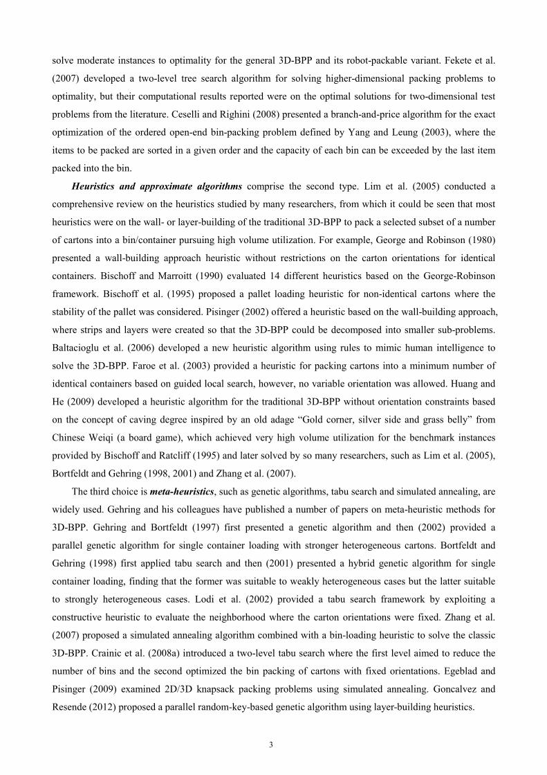
3.2.3 Detailed Decoding Procedure

Fig. 9 presents the detailed flowchart of the decoding procedure. To measure the quality of a packing

solution, volume utilization (Bischoff and Ratcliff, 1995) is quite often used by the researchers, which is

defines as:

%100])([1 ×××= HWLVF total (4)

where Vtotal is the total volume of the cartons, (L×W×H) is the volume of the bin used. We also note that Loh

and Nee (1992) used “packing density”, which is defined as:

%100)]([2 ×××= HWLVF cctotal (5)

where (Lc×Wc×H) is the volume of the final cage bin, the smallest rectangular box enveloping all the cartons

packed in the bin.

12

In this work, both F1 and F2 are used to measure the quality of a packing. F1 is equivalent to H, but F1 is

more distinctly to reveal the utilization rate of net space of the bin. Evidently, F2 reflects the real tightness of

the packing, hence should be used as one of the criteria to evaluate the performance the solution methods,

regardless of the argument that F2 overestimates the usual volume utilization (Bischoff and Ratcliff, 1995).

Table 4 presents the packing solution for the sample chromosome in Fig. 4, with the coordinates and

relative positions available.

i = 1

Get a chromosome Pj = (Pj1, Pj2), Pj1= (π1, π2, π3, …,

πN), Pj2 = (γ1, γ2, γ3, …, γN);

Change Pj into the carton list (c-list), each carton πi

obtaining a new dimension lni×wni×hni according to γi;

Put the original point (0, 0, 0) into the ref-point list, K=1;

Initial dimensions of the cage bin: lc=0, wc=0, hc=0.

k = 1, nf = 0

Fig. 9 The decoding procedure

nf = 0 ? N Y

N (xk+lni) ≤ L &

(yk+wni) ≤ W &

(zk+hni) ≤ H ?

Y

Check if carton

πi intersect with the other

packed cartons?

Mark point k (xk, yk, zk) as a feasible

reference point, nf +1, calculate the

index1 or index2 of this point.

N

Y

k + 1

k > K ? N

Y

Pack carton πi

upon the current

cage bin.

Based on index1 or index2,

choose the best point among

the nf points to pack carton πi.

Delete the occupied point

from the ref-point-list, K-1.

Try to parallel move carton πi in x, y and z

directions to make the packing more compact,

recording its final coordinates (xi, yi, zi) and its

left, front and bottom cartons in the c-list.

Add three new refrence points to the ref-point-

list, K+3. Update the dimension lc, wc and hc of

the cage bin.

i + 1

i > N ?

Output the packing with

its height H and filled

rates F1 and F2.

N Y

13

Table 4. The packing solution for the sample chromosome in Fig. 4

Original size New dimensions Coordinates Relative positions

i ππππi γi li wi hi lni wni hni xi yi zi left front bottom

1 1 1 36 36 36 36 36 36 0 0 0 0 0 0

2 10 1 33 21 4 33 21 4 0 0 36 0 0 1

3 6 4 40 31 21 31 21 40 0 36 0 0 1 0

4 8 4 31 17 16 17 16 31 31 36 0 6 1 0

5 3 5 54 40 21 21 54 40 0 0 40 0 0 10

6 5 3 52 33 20 33 52 20 21 0 40 3 0 10

7 2 6 59 39 20 20 39 59 54 0 0 5 0 0

8 9 4 26 23 14 23 14 26 48 39 0 8 2 0

9 7 5 31 31 17 17 31 31 36 0 0 1 0 0

10 4 1 58 37 21 58 37 21 21 0 60 3 0 5

L = 80, W = 58, H = 81, F1 = 74.33%; Lc = 79, Wc = 57, F2 = 76.60%

3.3 Sorting Heuristics and Random Search

Sorting the cartons according to certain rules has demonstrated some advantages in providing better

starting solutions for meta-heuristics. In fact, with the decoding procedure, we can conduct packing

simulation experiments to test the sorting heuristics of ordering the cartons. For instance, we can compare

the packing of the carton sequence in decreasing volume order and with various orientations. We also can

randomly search a large number of random solutions (chromosomes) within very short computational time

and select the best one for real packing. From the subsequent numerical experiments, we can see that the

random search combined with a sorting heuristic demonstrates better performance in solving large-size

packing problems than MILP model.

4. The Improved GA (IGA)

4.1 Tailored Components of IGA

4.1.1 Generation

At the beginning of the GA, an initial generation of chromosomes are often randomly generated. In IGA,

a new mechanism for producing the initial generation is designed considering both “first fit decreasing” and

diversity: (1) Six chromosomes with the same carton sequence in decreasing volume order, and each with an

orientation sequence of the same orientation γj, γj = 1, 2, 3, …, 6. That means, for each chromosome, the

cartons are packed in decreasing volume order and in the same orientation. Six orientations are exactly

covered by the six chromosomes. (2) The remainder chromosomes are produced randomly as usual.

Let popsize denote the number of individuals in the initial generation, which is a critical parameter to

control the solution quality, and is given according to problem size. At every iteration of GA, a new

generation is re-produced through crossover, mutation and selection, and popsize is usually kept constant.

4.1.2 Selection

Selection is the process to select most of the better individuals in each generation for crossover, part of

the generation (usually worse individuals) for mutation. Common selection methods include the

14

roulette-wheel selection (Goldberg, 1989) and the tournament method (Goldberg and Deb, 1991). The

tournament method is adopted in IGA due to the fact that in the tournament method the objective value of a

chromosome can be directly used as the selection criterion and thus time-saving.

In selection, the crossover and mutation rates are two crucial performance parameters that influence the

convergence speed of the GA. Assume the number of the chromosomes that are selected to crossover is xsize;

the number of the chromosomes that are selected to mutate is msize. The ratio Cr = xsize/popsize is called

crossover rate, often Cr∈[0.5, 0.9]; and the ratio Mr= msize/popsize called mutation rate, often Mr∈[0.1,

0.5]. In general, if Mr increases, GA will converge slowly, thus has more chances to approach better solutions;

but if Mr is too large, GA tends to behave like a random search.

4.1.3 Crossover

Crossover is the process during which two parents generate two offspring, such that the children inherit

a set of building blocks from each parent. Genetic operators are related to representation schemes. Poon and

Carter (1995) presented a survey of crossover operators for ordering applications. Regarding the

permutation-based representation, the following crossover operators have been widely used: partially

matched crossover (PMX) intending to keep the absolute positions of elements and linear order crossover

(LOX) intending to respect relative positions. In IGA, PMX is basically adopted for the carton sequences;

but for the orientation sequences, concomitant PMX is performed, so that the orientation of a carton is kept

unchanged, as shown in Fig. 10. The orientation change for a carton is implemented through the following

mutation operator.

4.1.4 Mutation

Mutation is the process to change some genes in a chromosome and produce a new chromosome. There

are also a number of methods to mutate (Gen and Cheng, 1997), such as reversion, swap and insertion.

He (2007 and 2009) has conducted a comparative study on reversion and swap mutations in solving

symmetrical and asymmetrical combinatorial problems, such as the traveling salesman problem (TSP) and

the zero-wait scheduling problems (ZWSP). According to our experience, it is evident that the swap mutation

is favorable to the problems with asymmetrical feature, especially in solving the large-size instances. The

3D-BPP is of highly asymmetrical feature, hence the swap mutation is found to be advantageous.

The mutation in this work has two functions: one is to change the order of the cartons to be packed; the

Two parents: 6 2 5 4 8 3 9 1 7 10 3 1 4 5 3 6 2 1 3 6

3 1 6 8 7 5 4 10 9 2 2 3 5 6 5 2 4 2 2 3

Fig. 10 Illustration of the process of concomitant PMX

6 2 3 8 7 5 4 1 9 10 3 1 6 6 5 2 4 1 2 6

5 1 6 4 8 3 9 10 7 2 2 3 4 5 3 6 2 2 5 3

Two offspring:

15

other is to assign new orientations for a carton. Following reversion or swap, random change of orientations

is conducted, making it possible for each carton to be packed in different orientations, and allowing the

algorithm to select the right orientation for a carton. Fig. 11 illustrates the mutation procedures. Considering

the following random change of orientations, the reversion or swap can be only carried out to the carton

sequence.

4.1.5 Termination Condition

Termination condition for IGA is that the algorithm stops when the objective value difference between

the worst chromosome and the best one in the current generation is equal to or less than a small value, like

0.1 or 0.01, which is dependent on the precision of the objective values.

4.2 Procedure of IGA

With GA components customized, the GA procedure is laid out as follows:

Step 1. Initial generation and evaluation: Produce an initial generation comprising popsize

chromosomes, and evaluate all the chromosomes using the decoding procedure.

Step 2. Selection: Select xsize better chromosomes in each generation to crossover, and msize worse

chromosomes to mutate.

Step 3. Crossover and Mutation: Conduct concomitant PMX to the xsize better chromosomes

generating xsize new chromosomes. Conduct mutation to the msize worse chromosomes generating msize

new chromosomes.

Step 4. Evaluation and new generation: The offspring (xsize+msize new chromosomes) from

crossover and mutation are decoded. Sort the parents and the offspring according to their objective values,

and select the former popsize best chromosomes as the new generation.

Step 5. Test the termination condition: If the termination condition is met, then go to Step 6; else go

Fig. 11 Illustration of the process of mutation

(a) Reversion and random change of orientations

8 2 1 4 6 9 3 5 7 10 1 5 6 5 2 3 1 6 2 3

8 2 1 3 9 6 4 5 7 10 1 5 6 1 3 2 5 6 2 3

8 2 1 3 9 6 4 5 7 10 1 2 6 1 4 2 5 3 2 3

5 1 6 3 8 4 9 2 7 10 5 3 4 2 3 6 2 6 4 1

5 1 2 3 8 4 9 6 7 10 5 3 6 2 3 6 2 4 4 1

5 1 2 3 8 4 9 6 7 10 4 3 6 2 1 2 2 4 5 1

(b) Swap and random change of orientations

16

to Step 2 for a new iteration.

Step 6. Output the results: Output the best chromosome and its corresponding packing solution.

4.3 Solution of SM00 by IGA

IGA, inclusive of the decoding procedure is

implemented in C language. Table 5 presents the

results of 10 runs of IGA for SM00, where the

parameter settings are popsize=200, xsize=160,

msize=40, with swap mutation used, and t denote the

iterations in each test l.

To evaluate the performance of meta-heuristics,

a number of computational tests are carried out. Each

test is one run of the algorithm with one final

solution. The relative deviation (denoted by RDl)

from the best solution of the tests is used to evaluate

each test, which is defined as:

%100])([ ×−= bestbestll HHHRD , (6)

where Hl is the objective value of the solution in test l, Hbest is the best of the tests. A lower average relative

deviation is generally expected.

5. The Global Search Framework for IGA

Besides the improvements on the genetic algorithm, the global search framework (GSF, He and Hui,

2010) is adopted to achieve better solutions for the large-size and highly heterogeneous packing problems. In

this framework, both evolved solutions and dynamic statistic information (the so-called evolutionary gradient)

are harnessed to guide the global search.

As well known, single meta-heuristic is problem dependent, its robustness is limited, and premature

convergence is another main drawback, especially for cases of large-scale problems. Hybridization,

parallelization and other search frameworks are the main effective measures to enhance the robustness and to

overcome the drawback of premature convergence. The proposed framework aims to address two issues: the

first goal is to solve larger problems within reasonable computational time; the second is to make the

algorithm more robust and less calibration effort. In fact, this framework has realized some parallel ideas in

the sequential environment.

It is well known that every run of the exact model for the same problem obtains the same solution; but

different runs of a meta-heuristic algorithm may obtain different solutions. That is why we often run the

meta-heuristic algorithm several times for the same problem and select the best solution for use. However, in

practical application, the user is more willing to run the packing program for only one time and then obtain

the expected packing solution.

Table 5. The results of 10 tests of IGA for SM00

Test l t CPU time (s) Hl RDl

1 29 0.187 72 1.408

2 23 0.109 76 7.042

3 28 0.110 74 4.225

4 28 0.109 75 5.634

5 18 0.078 77 8.451

6 23 0.094 74 4.225

7 25 0.094 76 7.042

8 35 0.140 71 0.000

9 30 0.125 76 7.042

10 26 0.094 76 7.042

Average 26.5 0.114 5.211

17

The distinction between the solutions from a number of computational tests is the impetus for us to

pursue much better solutions. In other words, the existing distinction implies that much better solutions are

possible if more computational tests are conducted. At the moment of seeing the distinction between the

solutions, what we should consider is how to effectively conduct the subsequent computational tests and

when to stop computing. Regarding these two questions, we proposed the concept of evolutionary gradient

and then devised a global search framework (He and Hui, 2010). In this framework, when the evolutionary

gradient vanishes, the algorithm stops. In this work, five scenarios of GSF are devised and tested, and the

best scenario is selected for the practical 3D packing problem.

5.1 Evolutionary Gradient

As well known, the concept of gradient is adopted in numerical methods, where the gradient is regarded

as the criterion to determine the termination of the algorithm – if the gradient turns to be zero, the optimum

or local optimum is deemed to have been found. Similarly, in evolutionary algorithms, the distinction

between the solutions obtained so far from computational tests can be treated as the criterion to determine the

termination of the algorithms, thus the concept of evolutionary gradient is proposed.

When a number of computational tests are carried out to evaluate the given algorithm, the relative

deviation (RD) of each test can be calculated with respect to the current best solution:

%100])[((%) ×−= bestcurrentbestcurrentvalueobjectiveRD . (7)

Let NL denote the number of computational tests of the single IGA. The mean relative deviation is defined as

evolutionary gradient, denoted by Edev:

∑=

=LN

l

l

L

dev RDN

E1

1, (8)

where RDl is the relative deviation of test l calculated by Eq. 7. In fact, Edev can be regarded as an important

sign which indicates whether it is necessary to conduct more computational tests for better solutions. If the

NL tests obtain solutions with the same objective value, then Edev = 0, which implies that it is not necessary to

carry out more tests; otherwise, Edev > 0, which indicates the probability of better solutions through

additional computational tests. The initial NL depends on the problem size. For large-size problems, we

usually witness Edev > 0, and additional runs are expected to provide better solutions. The additional NL can

be determined by the subsequent Eq. 9.

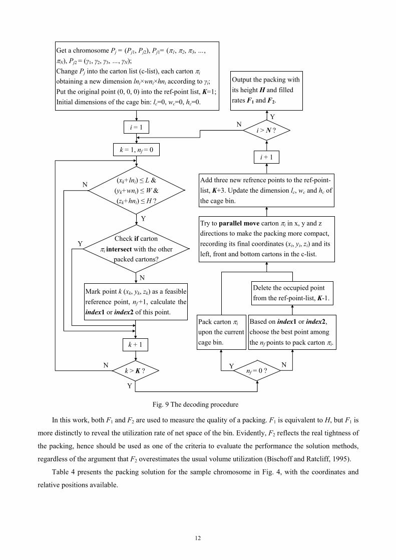
5.2 The Global Search Framework

Based on the concept of evolutionary gradient, three phases of computational tests are organized. In

phase 1, which is called rough search, NL tests of IGA are carried out to see whether the evolutionary

gradient exists (Edev > 0). If yes, go on with phase 2 which consists of one or more refining searches, each

refining search involves NL=f(Edev) tests of IGA, until the evolutionary gradient turns to be zero (Edev = 0).

Despite the zero evolutionary gradient approached at the end of phase 2, phase 3 can follow with further

ambition to find more refined solutions. In phase 3, if no new solution is found, only one refining search is to

18

be executed; otherwise, with new solution(s) obtained, several refining searches are to be conducted until the

new evolutionary gradient becomes zero. The rough search and refining searches can be considered as local

searches, while the whole organization of the three phases is called the global search framework. Each rough

search or refining search is seen as a global iteration, denoted by g; and a single IGA test as a local iteration,

denoted by l.

The procedure of the GSF is shown in Fig. 12(a). The rough search, as shown in Fig. 12(b), comprises

NL tests of IGA, each of which starts with an initial generation including the six heuristic chromosomes and

(popsize-6) random chromosomes, where the six heuristic chromosomes can be treated as excellent “breed”

or “seeds” to expedite the evolution. Each refining search, as shown in Fig. 12(c), comprises NL=f(Edev) tests

of IGA, each test starts with an initial generation including advanced chromosomes from last global iteration

and random chromosomes. NL = f(Edev) can be determined by Eq. 9,

f(Edev) =

−≥

+ ;,

11

,

LLLU

LLdev

devLL

LU

NN

NEif

EN

elseN (9)

where NLL and NLU are respectively the lower and upper bounds of the number of IGA tests. NL increases with

the decreasing of Edev, but has an upper bound. NL may also be set as a constant parameter in the search

process. In this work, NL is set as a constant number.

It should be emphasized that, in addition to GAs, other hybrid solution methods can also be

incorporated into the GSF. Using such a framework, much better solutions can be obtained in succession,

Fig. 12 Flow chart of the global search framework

(a) Global search framework

Rough search

Output the

best solution

g = 1

Calculate Edev(g) g + 1

Edev = 0 ?

Y

N Refining I or II

g + 1,

Calculate Edev(g)

Stop ?

Y

N Refining I

Edev = 0 ? Y N

(c) Refining search

NL=f(Edev)

IGA with advanced or

heuristic seeds

l = 1

l < NL? l + 1

N

Y

IGA with

heuristic seeds l = 1

l < NL?

l + 1

N

Y

(b) Rough search

19

until the evolutionary gradient vanishes.

5.3 Scenarios of GSF Considering Evolution Speed

The “refining I” and “refining II” in Fig. 12 are two kinds of refining searches with different breed of

selection strategies. For refining I, only the best solution found in iteration g is put into the initial generation

of each test in iteration g+1; but for refining II, all the NL evolved solutions obtained in iteration g are put

into the initial generation of each test in iteration g+1. For refining II, considering NL advanced seeds

introduced into a new evolutionary environment, it seems that the six heuristic seeds are not necessary to the

coming global iterations, and that NL can be reduced to a relative smaller number, both of which can expedite

evolution or solution speed. With these considerations, the scenarios presented in Table 6 are laid out for

simulation experiments to determine which one is the best. Subsequent numerical experiments demonstrate

that, in refining II, indeed NL can be reduced to a relative smaller number, but the six heuristic seeds are still

vital to the coming global iterations.

Table 6. Scenarios of GSF for simulation experiments

Scenario Option of phases 1, 2 or 3, refining I or II NL Heuristic seeds or not Performance

GGA1 Phase 1+2 (refining I): slow and nice solution 30 Yes ***

GGA2 Phase 1+2 (refining II): fast 10 No **

GGA3 Phase 1+2 (refining II): fast 20 No ***

GGA4 Phase 1+2 (refining II): fast and nice solution 20 Yes ****

GGA5 Phase 1+2 (refining II)+3 (refining I) 20 Yes *****

Furthermore, one may doubt the necessary existence of phase 3 in GGA5. For easy instances phases 1

and 2 are sufficient to obtain satisfactory solutions, indeed phase 3 additionally leads to another refining

search wasting some CPU time. However, for hard instances phase 3 gives rise to more chances to find much

better solutions. As known from the computational experiences in exact methods, even if the MILP model

has found the best solution to an instance, nevertheless, a long time is still needed to prove the optimality.

Compared with such a long time, the time for an additional refining search in phase 3 is very short.

5.4 Solutions of SM00 by GSF under Diverse Scenarios

Table 7 presents solutions of SM00 obtained under the various scenarios. GGA1 finds the best over a

longer time because of the bigger NL and only one advanced seed for further evolution. GGA2 has a short

time due to the smaller NL and NL advanced seeds for further evolution, but with a dissatisfactory solution.

The difference of GGA3 from GGA2 is only that NL is doubled, thus the solution is improved. In GGA2 and

GGA3, with NL advanced seeds for the coming global iterations, the evolution speed has indeed been

expedited. The difference of GGA4 from GGA3 is that, six heuristic seeds together with NL advanced seeds

are used for the coming global iterations, consequently further enhancing the evolution speed. GGA5 with

the merits of both GGA4 (fast speed) and GGA1 (ability for better solution) has found the best solution in

shorter time.

20

Table 7. Solutions of SM00 by GSF under diverse scenarios

Scenario NL G CPU time CT (s) H

GGA1 30 1+2=3 9.70 70

GGA2 10 1+2=3 2.91 72

GGA3 20 1+2=3 5.31 71

GGA4 20 1+2=3 4.95 71

GGA5 20 1+2+1=4 7.20 70

6. Computational Experiments

In this section, we apply the proposed methods to the cases solved in Wu et al. (2010), and expand the

experiments to some larger and more heterogeneous new cases. Moreover, GGA5 is tested with the

benchmark instances BR01~10 (Bischoff and Ratcliff, 1995).

6.1 Problem Data

In Wu et al. (2010), 10 packing cases of small bins (L×W×Hmax=80×58×95 for SM04 and SM05, and

L×W×Hmax=78×57×95 for other small cases) and 27 cases of big bins (L×W×Hmax=116.5×97×95) were

collected from a company where the workers manually pack cartons in the bin based on a rule of thumb and

their own packing experience. In these cases, there exist 13 types of cartons, each case involves no more than

9 types of cartons, and the number of cartons to be packed into a bin is no more than 40 (N ≤ 40). We denote

the original GA in Wu et al. (2010) as OGA.

The new cases in this work include 6 packing cases of small bins (L×W×Hmax=80×58×95) and 12 cases

of big bins (L×W×Hmax=116.5×97×95). In contrast to the old small-bin cases which contain 3 ~ 5 carton

types, the new small-bin packing involves 8~11 carton types; and each new big-bin case involves 7~13

carton types instead of 2~9 carton types for the old big-bin cases. For the new cases, up to 40 cartons are

loaded into a small bin, and up to 80 cartons are packed into a big bin.

To evaluate the performance of the methods for more heterogeneous instances, two particular big-bin

packing cases, BM40 and BM41, are tested. In BM40 and BM41, 20 cartons to be packed involve 20 carton

types, i.e., each carton belongs to a different carton type.

6.2 Algorithm Parameter Setting

The IGA and the global search framework are coded in C language and compiled with Microsoft Visual

VC++ 8.0. All the numerical experiments are conducted on a computer with an Intel T7500 2.20GHz Duo

CPU and 1.96GB RAM.

Parameter setting is an important issue which impacts the performance. In the GA, the setting of the

population size (denoted by popsize) in a generation depends on the problem size. The crossover rate (Cr)

and mutation rate (Mr) are two crucial factors that influence solution quality and convergence speed. In the

GSF, the number (NL) of IGA tests within a global iteration is also an important parameter to determine the

solution time and quality.

In OGA, Mr is given differently according to the mutation methods, reversion (Rvs) or swap (Swp), and

21

a fixed number of iterations (denoted by iter.) is set for each OGA test. Specifically, in OGA with Rvs

mutation, (popsize, Cr, Mr, iter.) = (120, 0.9, 0.5, 200) for small-bin cases (SM), and (200, 0.9, 0.5, 500) for

big-bin cases (BM); in OGA with swap mutation, (popsize, Cr, Mr, iter.) = (120, 0.9, 0.9, 200) for SM, and

(200, 0.9, 0.9, 500) for BM. A notable setting of Mr is that it was set up to 0.9! The best solution by OGA is

selected from 20 computational tests.

In IGA, Mr has been tuned from 0.1 to 0.5, with decreasing convergence speed, but not improving the

solution quality so much, thus Mr is given as 0.2. Due to the termination condition of until-no-improvement

adopted in IGA, the computation of the algorithm stops at the iteration of “no improvement”. So in IGA,

(popsize, Cr, Mr) = (200, 0.8, 0.2) for SM, and (400, 0.8, 0.2) for BM. The best solution by IGA is also

selected from 20 computational tests.

In the different scenarios of GSF, (popsize, Cr, Mr) = (200, 0.7, 0.3) for SM, and (400, 0.7, 0.3) for BM,

with a little change of Cr and Mr to allow the algorithms to search more combinations of carton orientations.

NL is set as 30 for GGA1, 10 for GGA2, 20 for GGA3, GGA4 and GGA5.

We also list the search results by the MILP, the manual packing (when possible) and a controlled

random search. The MILP model is limited by a running time of 7200 seconds (two hours). In the random

search (Rdm) combined with sorting heuristics based on the decoding procedure, 500 feasible solutions are

searched for SM, 1000 for BM, including the six heuristic solutions.

6.3 Results and Analysis

With the parameter setting, numerical experiments have been performed. The comparative study is

carried out from three aspects: the packing height (H), filled rates (F1 and F2) and computational time (CT).

Tables 8 and 9 show the best solutions (H) of the cases obtained via a range of methods or scenarios. The

best solution for an instance by OGA or IGA is selected from 20 computational tests, so the computational

time for OGA or IGA is the total running time of the 20 tests. The other methods, including the random

search, MILP and the scenarios of GSF, obtain the best or optimal solution for an instance at the end of their

execution. Tables A-1 to A-5 in Appendix A provide the corresponding filling rates and computational times

of these methods.

6.3.1 Comparison of Packing Height

From Tables 8 and 9, the following observations can be noted:

(1) Random search vs. manual packing. For the old cases, the manual packing heights are presented

in Table 8. Compared with the manual packing, the random search has found better solutions for 22 cases

among the 37 cases. Moreover, from filled-rate comparison (see Table A-1), it is noted that the random

search gets a higher average F1 than the manual packing. The random search is completed within one second

for the old cases, or within 3 seconds for new cases (see Tables A-4 and A-5). For the moderate size

instances (BM13~27), the random search approaches almost the same average F1 as the manual packing.

Hence, for the new cases where the manual packing data are not available, the results by the random search

are treated as the ones by the manual packing.

22

(2) Reversion mutation vs. swap mutation: Both in OGA and IGA, the two mutation methods have

compared, and corresponding results are presented in Tables 8 and 9 from which it is verified again that

swap mutation is more favorable to the solution quality of the algorithms.

(3) IGA(swp) vs. OGA(swp). IGA(swp) performs better than OGA(swp) both in solution quality and

speed. For 31 cases among the 55 cases, IGA(swp) finds better solutions than OGA(swp). Only for BM24,

IGA(swp) obtains a worse solution than OGA(swp).

(4) Different scenarios of GSF: Five scenarios of GSF as shown in Table 6 are also tested with all the

cases to reveal their performance in solving diverse instances. The experiment results show that GGA1 and

GGA4 have complementary merits: GGA1, further refining searches (local search actually) with one evolved

solution consecutively, can find good solutions but with longer search time; GGA4, further refining searches

with a number of evolved solutions consecutively, can obtain good solutions with higher speed. GGA5, first

conducting refining searches with a number of evolved solutions and then with one evolved solution, has the

merits of both GGA4 and GGA1, thus has found new solutions for most of the cases. For SM04, SM06 and

SM10, GGA5 finds the same proven optimal solutions as MILP model, but the other GA-based methods

have not found these solutions.

(7) GGA5 vs. GAs. For most of the instances, the GGA5 has achieved better solutions than OGA (see

Tables 8 and 9, better solutions by GGA5 vs. OGA are marked with #), but the computational times are much

shorter (see Tables A-4 and A-5). Only the solution (H = 97) for SM15 by GGA5 exceeds Hmax, leaving this

instance as a challenge for coming work. Furthermore, compared to IGA, GGA5 has achieved better

solutions for almost all of the new cases (see Table 8, better solutions by GGA5 vs. IGA are marked with $),

which demonstrates that the GSF actually helps improve the solution quality, especially in solving the large-size

cases.

23

Table 8. The best solutions (heights) of the old cases by different methods MILP

OGA IGA GSF

N Manual Rdm MILP& Rvs Swp Rvs Swp GGA1 GGA2 GGA3 GGA4 GGA5

SM01 8 91 92 80* 80 80 80 80 80 80 80 80 80

SM02 8 56 40 37* 37 37 37 37 37 37 37 37 37

SM03 9 69 53 47* 47 47 47 47 47 47 47 47 47

SM04 9 91 103 82 83 83 83 83 82 83 83 83 82#

SM05 10 56 61 52* 52 52 52 52 52 52 52 52 52

SM06 12 53 48 38* 40 40 40 40 40 40 40 40 38#

SM07 17 70 62 62 62 62 62 62 62 62 62 62 62

SM08 17 91 77 71 68 69 64 62 62 64 62 62 62#

SM09 19 71 62 62 52 52 51 51 51 51 51 51 50#

SM10 21 85 78 62 64 63 64 63 62 63 62 62 62#

BM01 5 91 84.1 84.1* 84.1 84.1 84.1 84.1 84.1 84.1 84.1 84.1 84.1

BM02 11 91 99 83.1 84.1 84.1 84.1 84.1 84.1 84.1 84.1 84.1 84.1

BM03 12 45 47 32* 32 32 32 32 32 32 32 32 32

BM04 13 91 98 77.4 83.4 83.4 83.4 77.4 77.4 79 77.4 77.4 77.4#

BM05 15 91 90 79 80 79 80 79 78 79 79 78 78#$

BM06 16 67 47 40 40 40 40 40 40 40 40 40 40

BM07 21 48 40 40 38 40 38 38 37 37 37 37 37#$

BM08 22 59 54 53 53 51 53 51 48 51 50 48 48#$

BM09 23 94 80 82 71 72 72 71 71 71 71 71 71#

BM10 23 91 62 63.1 61 61 61 61 61 61 61 61 61

BM11 25 91 80.1 78 73.4 77.4 73.4 73.4 73.4 73.4 73.4 73.4 73.4#

BM12 26 94 66 68 61 61 61 61 61 61 61 61 61

BM13 27 83 85 78 73 71 69 69 68 70 69 68 68#$

BM14 28 95 94 88.4 79 78.4 78.4 78.4 78.4 80 78.4 78.4 78.4

BM15 29 91 94 87 77 75 75 74 74 74 73 73 73#$

BM16 29 63 54 52 48 48 47 47 47 47 47 47 47#

BM17 29 91 101 88.4 82 80 79 78.4 78.4 79 80 80 78.4#

BM18 30 70 70 73.4 67 63.1 63 63 63 63 63 63 63#

BM19 30 94 78.4 79 63.4 63.1 63.4 63.1 63 63 63 63 63#$

BM20 30 94 94 87 80 79 79 79 78 80 78 78 78#

BM21 30 95 94 87 82 78.4 78.4 78.4 78.4 78.4 78.4 78.4 78.4

BM22 31 91 85 87 78 78 78 78 77 78 78 77 77#$

BM23 33 95 94 93.4 78 78.4 78 77.4 77.4 77.4 77.4 77 77#$

BM24 35 91 94 89 84.1 80 81 82 79 85 79 85 79#$

BM25 36 94 87 79 76 76 75 73 75 77 71 71 71#$

BM26 38 91 101 97 85 82 80 80 80 80 80 80 80#

BM27 40 91 100 109 85 85 84 85 84 84 85 84 84#$ & Solved by CPLEX 11.2;

* Proven optimal solution;

# New solution compared to OGA;

$ New solution compared to IGA.

24

Table 9. The best solutions (heights) of the new cases by different methods

OGA IGA GSF

N Rdm MILP& Rvs Swp Rvs Swp GGA1 GGA2 GGA3 GGA4 GGA5

SM00 10 80 68* 72 72 72 71 70 72 71 71 70#$

SM11 11 96 80 84 88 83 83 80 83 80 83 80#$

SM12 20 110 90 89 89 89 89 89 90 89 89 87#$

SM13 20 113 104 98 98 98 95 95 98 97 96 94#$

SM14 31 109 105 91 91 90 90 90 90 89 89 89#$

SM15 40 126 118 106 103 100 100 98 100 100 100 97#$

BM28 13 77.4 61 64 64 63.1 63.1 61 63.1 61 61 61#$

BM29 30 106 100 90 89 91 89 89.4 90 89.4 87.4 87.4#$

BM30 35 96 99 89 85 86 85 85 84 83 83 83#$

BM31 40 87 98 78 78 78 76 76 78 78 76 75#$

BM32 45 99 102 97 89 90 88 88 89 89 89 88#

BM33 50 88 95 76 73 72 71 71 71 71 71 70#$

BM34 55 108 116 99 96 94 94 93 94 91 91 90#$

BM35 60 86 95 81 78 74 74 73 74 74 74 73#$

BM36 65 91 104 87 83 83 82 80 82 81 81 79#$

BM37 70 105 112 91 89 88 88 86 88 87 88 86#$

BM38 75 96 107 91 90 88 88 86 88 87 86 86#$

BM39 80 107 121 102 95 93 93 90 92 90 90 90#$

BM40 20 107.4 96 90 92 91 91 90 90 90 90 90#$

BM41 20 103.1 87 86 85.4 85 85 84.1 85.4 85 85.4 84.1#$ & Solved by CPLEX 11.2;

* Proven optimal solution;

# New solution compared to OGA;

$ New solution compared to IGA.

6.3.2 Comparison of Filled Rates F1 and F2

Tables A-1~3 show the filled rates comparison of the methods. As defined in §3.2.3, F1 is calculated

with respect to the net volume of the bin used, while F2 is calculated with respect to the volume of the final

cage bin, which reflects the actual degree of the packing tightness.

With the packing height H available and given L×W of the bin, and the total volume of the packed

cartons, F1 can be calculated using Eq. 4. But to calculate F2 with Eq. 5, Lc×Wc of the cage bin has to be

given. For manual packing with only the height H, rather than the detailed solution with coordinates (x, y, z),

Lc×Wc is impossible, hence F2 is not given for manual packing. For the solutions by MILP and OGA, a

conversion program is designed to change the solutions into new format with F1, F2 and relative position. For

the MILP model, it is found that most of them have the equal F1 and F2. This phenomenon is plausible from

the constraints and the Big-M used in the MILP model. The results by the random search are to be compared

with those by manual packing and MILP, thus without F2 presented.

The cases studied can be categorized into five groups as listed in Table 10, where the old cases are

divided into two groups, and the new cases into three groups.

25

Table 10. Groups of the cases studied

Group Cartons N Bin Type Results Old or New Cases

1 N ≤ 26 small or big-bin Tables 8, A-1, A-4 old

2 27 ≤ N ≤ 40 big-bin Tables 8, A-1, A-4 old

3 10≤N≤40 small-bin and

BM28, BM40, BM41 Tables 9, A-2, A-5 new

4 30≤N≤80 big-bin Tables 9, A-2, A-5 new

5 10≤N≤20

Heterogeneous small or big-bin Tables 9, A-3, A-5 new

The old cases in Table A-1 can be classified into two groups, group 1 (N ≤ 26) with a small

number of cartons to be packed, group 2 (27≤ N ≤40) with a moderate number of cartons.

In group 1 (N ≤ 26), a lower average F1 (65.68% for small-bin packing and 65.71% for big-bin

packing) by the manual operation for both small-bin packing and big-bin packing; as a contrast, the

random search achieves a higher average F1 (72.05% and 74.25%). In group 1, MILP model can

obtain much higher average F1 (81.99% and 81.06%) than the random search. The average F1 by OGA

(82.88% and 82.61%) and IGA (83.99% and 83.95%) increases a bit. The average F1 by GGA5

(84.84% and 84.64%) increases about 2% against OGA. Fig. 13 shows the situation of the average F1

for group 1, where it can be seen that MILP, OGA, IGA and GGA5 increase F1 by 15%~ 19% with

respect to the manual packing.

In group 2 (27≤ N ≤40), the packing by the manual operation, the random search and MILP

model has similar lower average F1 (74.31%, 74.48% and 77.73% respectively); but OGA, IGA and

GGA5 increase by 14%~16% with respect to the manual packing. For these moderate-size instances,

our random search obtains almost the same average F1 as the manual packing. That is why the packing

solutions by the random search for the new cases can be regarded as the real manual packing solutions.

It should be noticed is that GGA5 achieves up to an average F1 of 90%. Fig. 14 shows the situation of

the average F1 for group 2. It is obvious that GA-based methods take great advantage over the others.

Fig. 13 Average F1 for small-size old cases (group 1) Fig. 14 Average F1 for moderate-size old cases (group 2)

ManualManualManualManual

RdmRdmRdmRdm

MILPMILPMILPMILP

GGA5GGA5GGA5GGA5

IGAIGAIGAIGA

OGAOGAOGAOGA

65656565

70707070

75757575

80808080

85858585

Manual Rdm MILP OGA IGA GGA5

Average F1(%

)

Small-bin packingSmall-bin packingSmall-bin packingSmall-bin packing

Big-bin packingBig-bin packingBig-bin packingBig-bin packing

ManualManualManualManual RdmRdmRdmRdm

GGA5GGA5GGA5GGA5IGAIGAIGAIGA

OGAOGAOGAOGA

MILPMILPMILPMILP

70707070

75757575

80808080

85858585

90909090

Manual Rdm MILP OGA IGA GGA5

Average F1(%

)

26

Fig. 15 Average F1 for small-size new cases (group 3) Fig. 16 Average F1 for large-size new cases (group 4)

The new cases in Table A-2 can also be classified into two groups: the small-bin packing cases

(10≤N≤40) and the big-bin cases (BM28, BM40 and BM41) with more heterogeneous cartons

(13≤N≤20) are put into group 3 (small-size instances in Table A-2), the big-bin packing cases

(BM29~39) with a large number of cartons are put into group 4 (30≤N≤80 in Table A-2, big-bin

packing).

In group 3, the situation of the average F1 is similar to group 1, it is also can be seen that MILP,

OGA, IGA and GGA5 achieve higher average F1 (83%~90%, see Fig. 15).

The situation of group 4 varies: the MILP model’s performance declines severely. For this group

of large-size instances, OGA, IGA and GGA5 demonstrate distinct advantage over the other

techniques, as shown in Fig. 16.

Table A-3 provides statistic results of the heterogeneous

cases in which each carton belongs to a different carton type.

These cases are put into group 5 (with 10≤N≤20 different

cartons). For this group, MILP shows its dominance with

higher average F1 over OGA and IGA. However, GGA5 is

still the best! Fig. 17 shows the situation of the average F1

for group 5.

From group 1 to group 5, IGA obtains higher average

F1 than OGA, and GGA5 higher than IGA logically and rationally. Another observation worth

noticing is that, when OGA and IGA obtain the same packing height (H) for a packing case, thus the

same value of F1, but IGA achieves higher value of F2 than OGA (see the cases SM01, 07 and 10,

BM02, 06, 08, 10, 12, 14, 19~22, 27, 29 and 30, totally 16 cases). That means IGA pack cartons much

tighter than OGA owing to the improved decoding procedure, especially because of index2 and new

parallel moving strategy adopted.

RdmRdmRdmRdm

MILPMILPMILPMILP

OGAOGAOGAOGA

GGA5GGA5GGA5GGA5

IGAIGAIGAIGA

70707070

75757575

80808080

85858585

90909090

Rdm MILP OGA IGA GGA5

Average F1(%

)

Small-bin packingSmall-bin packingSmall-bin packingSmall-bin packing

Big-bin packingBig-bin packingBig-bin packingBig-bin packingRdmRdmRdmRdm

MILPMILPMILPMILP

GGA5GGA5GGA5GGA5

IGAIGAIGAIGA

OGAOGAOGAOGA

70707070

75757575

80808080

85858585

90909090

Rdm MILP OGA IGA GGA5

Average F1(%

)

RdmRdmRdmRdm

MILPMILPMILPMILP

GGA5GGA5GGA5GGA5

IGAIGAIGAIGA

OGAOGAOGAOGA

70707070

75757575

80808080

85858585

90909090

Rdm MILP OGA IGA GGA5

Average F1(%

)

Fig. 17 Average F1 for heterogeneous group 5

27

6.3.3 Comparison of Computational Time

Computational time is an important factor to evaluate an algorithm. Tables A-4 and A-5 present

the computational times (CT) of five methods in solving the old and new instances, and the time is in

seconds. From these two tables, we can see the following facts:

(1) The random search based on the decoding procedure can be finished within very short time

(CTR < 3s). So the decoding procedure can be used for packing simulation experiments conveniently.

(2) For most cases, MILP model reach the limited running time, 2 hours (7200s). Taking the

volume utilization into account, MILP model can only find satisfactory solutions for the small-size

instances in groups 1, 3 and 5 within the limited time.

(3) The solution speed of IGA is about 14 times faster than that of OGA. From the comparison of

filled rates, IGA achieves higher filled rates (F1 and F2) than OGA.

(4) The solution speed of GGA5 is about 4 times faster than that of OGA. What is more, GGA5

improves the average F1 by approximate 2~4% with respect to OGA. When OGA is applied to the

large-size instances BM37, 38 and 39, the solution times are 8437 seconds (2 hours and 20 minutes),

11189 seconds (about 3 hours), 14601 seconds (about 4 hours) respectively, all over 2 hours. But for

these three cases, GGA5 has completed the search within 2016 seconds (about 33 minutes).

(5) The average number of global iterations g in GGA5 is about 4 (3.84 for the old cases, 4.45 for

the new cases). For the cases BM08, BM24 and SM15, the global iterations g of GGA5 are 6, 9 and 7

respectively. These data reveal the fact that the global iterations of GGA5 are indeed essentially

necessary to achieve the high quality solutions.

6.3.4 Comprehensive Comparison

From the comparison and analysis of the packing height (H), filled rates (F1 and F2) and

computational time (CT), the following comprehensive recognitions can be drawn out:

(1) The random search has an equal or even higher average F1 than the manual packing, with very

short search time (less than 3 seconds). This means that the decoding procedure is effective in

simulating a packing solution.

(2) MILP model can only obtain satisfactory solutions for the small-size instances (N≤26) within

acceptable time (e.g. 2 hours); but for moderate-size or large-size instances, the exact model, which is

limited by the current computing resources, such as computational time, memory and CPU speed,

shows its apparent inferior position in contrast to the GA-based methods.

(3) OGA is indeed effective and efficient in solving the original small- and moderate-size

instances, but has still left a larger space for further improvement. For the new cases including more

heterogeneous cases, OGA shows its drawbacks in terms of solution speed and quality. As a contrast,

IGA witnesses improvement not only on solution speed but also on solution quality.

(4) The novel GSF (GGA5) has obtained the best solutions for most of the old and new cases

28

among the methods tested, within acceptable time (less than 33 minutes), hence is the best method

tested in our work.

It should also be mentioned that in Wu et al. (2010), the achieved bin height for each test case was

fed into the container loading algorithm provided by Martello et al. (2007) for runs of two hours. In

most cases, the Martello et al. (2007) code was not able to provide a solution to load all the cartons

within the given height limit. Since the results provided in this paper are better than those of Wu et al.

(2010), it can be reasonably concluded that it would be even more difficult for the algorithm described

in the Martello et al. (2007) to provide feasible results under the same settings in Wu et al. (2010).

6.4 Tests on 3D-SPP Benchmark Instances

6.4.1 Result Comparison

As explained earlier, the problem proposed in this paper is similar to the 3D-SPP but has some

distinct features. For heuristics algorithms, it is common to exploit the problem features to ensure

effectiveness and efficiency. Although the proposed algorithms did not take 3D-SPP into consideration

at the design phase, one of the algorithms, GGA5, is applied to testify its effectiveness on some of the

strip packing instances from Bischoff and Ratcliff (1995) as an additional way for benchmarking. We

have to mention that the use of genetic algorithms actually has some challenges when the number of

cartons to be packed increases and therefore the tests on the 3D-SPP benchmarking instances can be

viewed as a ‘stretch’ for the current algorithms. We first apply the GGA5 to the selected 3D-SPP cases

without imposing the orientation constraints (marked as ‘w/o orient. con.’) and subsequently consider

the orientation constraints (marked as ‘with orient. con.’) in both generating chromosomes and

mutating according to the specified orientation constraints, where the GA parameters remain the same,

(popsize, Cr, Mr) = (400, 0.7, 0.3). We then compare the results with those presented in Bortfeldt and

Mack (2007) and Allen et al. (2011) where some of the state of the art results are available. We also

notice that a working paper by Bortfeldt and Jungmann (2010) has seemingly improved the results

significantly. Table 11 shows the volume utilization (F1) for all these methods.

For GGA5, most of the cases where the orientation constraints are not imposed generate slightly

better results than those with orientation constraints imposed, except for BR03 and BR10. Look across

GGA5 with orientation constraints, Bortfoldt and Mark (2007) and Allen et al. (2011), the volume

utilizations achieved by GGA5 for BR01~03 and BR05 are higher than those obtained by Bortfeldt

and Mack (2007) and Allen et al. (2011). We also get close results for the rest cases. In terms of overall

average volume utilization, ours is also higher than that of Bortfeldt and Mack (2007) and Allen et al.

(2011). Computational time wise, ours is longer than that of Bortfeldt and Mack (2007) and Allen et al.

(2011) due to operations involved in the genetic algorithms. The results from Bortfeldt and Jungmann

(2010), where the algorithm tries to solve a series of container loading problems iteratively (in reduced

length), seem to be the best among all methods presented in Table 11.

29

Table 11. Results for the test cases BR01~10 from Bischoff and Ratcliff (1995)

GGA5 F1 (%) Types N

w/o orient. con. with orient. con.

B&M (2007)

F1 (%)

Allen et al. (2011)

F1 (%)

B&J (2010)

F1 (%)

BR01 3 139.4 91.70 91.52 87.3 90.0 94.2

BR02 5 140.1 91.85 90.84 88.6 89.6 94.8

BR03 8 135.4 90.53 90.53 89.4 89.9 94.7

BR04 10 132.2 90.31 89.49 90.1 88.8 94.2

BR05 12 127.8 89.91 89.57 89.3 88.5 93.9

BR06 15 133.8 89.75 89.47 89.7 88.6 93.5

BR07 20 129.2 88.59 88.23 89.2 88.7 92.6

BR08 30 138.0 87.44 87.32 87.9 88.3 91.8

BR09 40 127.5 86.54 86.19 87.3 87.9 91.5

BR10 50 129.2 86.30 86.41 87.6 87.9 91.3

Average 19.3 133.3 89.29 88.96 88.64 88.82 93.2

6.4.2 Difference Analysis

In terms of measuring difficulty of packing problems, Smith-Miles and Lopes (2012) review

some common combinatorial optimization problems. One particular factor proposed for bin packing in

that paper is the average carton volume against the bin volume as one of the measurements for

difficulty. Fig. 18 presents the carton volume against the bin volume for each carton in cases of SM14,

BM31, BM39, BR06-008 and BR10-009. It can be observed that in terms of number of cartons for

packing, SM13 and BM34 (and most other cases investigated in this paper) represent a category of

problem with relatively small number of cartons but significantly differ in terms of carton sizes and

number of cartons available per carton type. On the contrary, BR06-008 and BR10-009 represent

typical strip packing problems, where more cartons are to be packed and each carton type usually

includes quite a number of cartons; moreover, the size difference between types is relatively lower.

These features were effectively utilized by the algorithms proposed in Bortfeldt and Mack (2007) and

Allen et al. (2011), and other algorithms with effective layer-packing and strip building.

Fig. 19 further indicates the difference between our investigated cases and those of traditional

3D-SPP, where the maximum, minimum and average carton volumes against the ‘bin’ (container)

volume are presented. It can be observed that the maximum cartons in some selected cases from this

paper have a volume that is more than 20% of the ‘bin’ itself; most of the maximum cartons are more

than 10% of the ‘bin’ volume, while none of the cases selected from BR01 to BR10 has a carton

volume more than 3% of the overall container volume.

30

0%

2%

4%

6%

8%

10%

12%

1 6 11 16 21 26 31 36 41 46 51 56 61 66 71 76 81 86 91 96 101 106

SM14

BM31

BM39

BR06-008

BR10-009

Fig. 18 Carton vs. bin volume comparison for SM14, BM31, BM39, BR06-008 and BR10-009

0%

5%

10%

15%

20%

25%

30%

BM04 SM06 BM16 BM13 BM39 BM24 SM14 SM11 BM31 BM30 BM28 BM29 BM41

Min

Max

Avg

0%

1%

2%

3%

4%

5%

BR01-009

BR02-001

BR03-001

BR04-001

BR05-001

BR06-008

BR07-007

BR08-007

BR09-009

BR10-009

Min

Max

Avg

(a) Cases from this paper (b) Cases from BR01 to BR10

Fig. 19 Maximum, minimum and average volume against ‘bin’ volume

7. Conclusion

This study, with the aim to solve the challenging real-world 3D packing problem with variable

carton orientations, has made meticulous improvement to the packing (decoding) procedure, devised a

particular genetic algorithm with customized selection, crossover and mutation operators, and adopted

a novel global search framework based on the concept of evolutionary gradient. The numerical

experiments indicate that the selected scenario of the global search framework is able to solve the

investigated packing problem effectively and efficiently. The novelty and contribution of this work can

be summarized as follows:

(1) A novel index (index2) is defined for the selection of reference points in locating a carton in

the bin, which is the crucial reason that makes the packing more compact.

(2) A new parallel moving strategy is proposed to reduce possible gaps and to avoid apparently

31

invalid moves thus save computational time and provide faster and more compact packing.

(3) The relative positions which indicate the cartons that are touched on the left, in front and at

the bottom of a particular carton can be reported via the improved decoding procedure. This, to our

knowledge, is the first attempt to presenting relative positions, which provides to be very convenient

and handy to guide manual packing in practice.

(4) Appropriate genetic components have been selected and well combined together with

simultaneous consideration of solution speed and precision.

(5) The concept of evolutionary gradient has been proposed considering the usual existing

diversity of the solutions obtained by meta-heuristics, e.g. the genetic algorithm. The global search

framework has subsequently been devised in order to make full use of the solution ability of the

selected genetic algorithm.

(6) Several scenarios of the GSF have been constructed and examined with the purpose to

improve the solution speed. A suitable scenario (GGA5) has then been selected and tested with a wide

range of packing cases, including larger-size and more heterogeneous instances. For most of the

instances, the GGA5 has achieved better solutions than OGA, and the computational times are much

shorter.

With the above novelty, the GSF is able to achieve packing solutions with average volume

utilization up to 85~90% within half an hour; for some cases, the volume utilization reaches

92~95%. In contrast, the manual packing only has average volume utilization less than 75%, with

very few exceptional cases reaching 80~82%. The average increment of volume utilization by GGA5

can be more than 15% against the current practical operations.

To sum up, the GSF can provide high-fill-rate packing solutions with information of the relative

positions, orientations and coordinates of the cartons. Furthermore, with the ability to handle arbitrary

orientations and heterogeneous cartons, the proposed method can be easily tailored and applied to

other types of bin packing problems.

The GSF can be easily transformed into a synchronous parallel version, because the

synchronization and communication, which are the difficult issues in parallel computing, are already

available. The further interesting work is to design an asynchronous parallel version of this

framework.

Acknowledgement

The authors would like to acknowledge Emerson Singapore Distribution Center for providing the

operational packing data, and give our special thanks to Mr. Jack Wong and Mr. Andy Chang.

The authors would also like to thank the anonymous reviewers for their constructive and pertinent

comments, which have significantly improved the paper into its current form.

32

References

Allen, S. D., Burke, E. K. and Kendall, G. 2011. A hybrid placement strategy for the three-

dimensional strip packing problem. European Journal of Operational Research, 209, 219–227.

Baltacioglu, E., Moore, J. T., Hill Jr., R. R. 2006. The distributor’s three dimensional pallet-packing

problem: a human intelligence-based heuristic approach. International Journal of Operational

Research 1, 249–266.

Bean, J. 1994. Genetic algorithms and random keys for sequencing and optimization. ORSA Journal

on Computing 6, 154–60.

Bortfeldt, A. and Jungmann, S., 2010. A tree search algorithm for solving the multi-dimensional strip

packing problem with guillotine cutting constraint. Working paper. Accessed on 01 October 2011,

URL: ftp://ftp.fernuni-hagen.de/pub/fachb/wiwi/winf/forschng/publi/DBFakWiWi458.pdf

Bortfeldt, A. and Mack, D., 2007. A heuristic for the three-dimensional strip packing problem.

European Journal of Operational Research, 183, 1267–1279.

Bischoff, E. E., Janetz, F., Ratcliff, M. S. W. 1995. Loading pallets with non-identical items.

European Journal of Operational Research 84, 681–692.

Bischoff, E. E., Marriott, M. D. 1990. A comparative evaluation of heuristics for container loading.

European Journal of Operational Research 44, 267–276.

Bischoff, E. E., Ratcliff, M. S. W. 1995. Issues in the development of approaches to container loading.

OMEGA—International Journal of Management Science 23, 377–90.

Bortfeldt, A. , Gehring, H. 1998. Applying tabu search to container loading problems. In: Operations

research proceedings. Berlin: Springer Press, 533–538.

Bortfeldt, A., Gehring, H. 2001. A hybrid generic algorithm for the container loading problem.

European Journal of Operational Research 131, 143–161.

Ceselli, A., Righini, G. 2008. An optimization algorithm for the ordered open-end bin-packing

problem. Operations Research 36, 425–436.

Chen, C. S., S. M. Lee, Q. S. Shen. 1995. An analytical model for the container loading problem.

European Journal of Operational Research 80, 68–76.

Crainic, T. G., Perboli, G., Tadei, R. 2008a. TS2PACK: A two-level tabu search for the three-

dimensional bin packing problem. European Journal of Operational Research. In press.

Crainic, T. G., Perboli, G., Tadei, R. 2008b. Extreme point-based heuristics for three- dimensional bin

packing. INFORMS Journal on Computing 20, 368–384

den Boef, E., J. Korst, S. Martello, D. Pisinger, D. Vigo. 2005. Erratum to “The three-dimensional bin

packing problem”: Robot-packable and orthogonal variants of packing problems. Operations

Research 53, 735–736.

Dosa, G. 2007. The tight bound of first fit decreasing bin-packing algorithm is FFD(I)

≤11/9OPT(I)+6/9. In: Combinatorics, Algorithms, Probabilistic and Experimental Methodologies,

volume 4614 of LNCS, pages 1–11. Springer, Berlin.

Egeblad, J., Pisinger, D. 2009. Heuristic approaches for the two- and three- dimensional knapsack

packing problem. Computers & Operations Research 36, 1026–1049.

Fanslau, T. and Bortfeldt, A. 2010. A tree search algorithm for solving the container loading problem.

INFORMS Journal on Computing, 22, 222–235.

Faroe, O., Pisinger, D., Zachariasen, M. 2003. Guided local search for three- dimensional bin-packing

33

problem. INFORMS Journal on Computing 15, 267–283.

Fekete, S. P., Schepers, J., van der Veen, J. C. 2007. An exact algorithm for higher- dimensional

orthogonal packing. Operations Research 55, 569–587.

Gehring, H., Bortfeldt, A. 1997. A genetic algorithm for solving the container loading problem.

International Transactions in Operational Research 4, 401–418.

Gehring, H., Bortfeldt, A. 2002. A parallel genetic algorithm for solving the container loading problem.

International Transactions in Operational Research 9, 497–511.

Gen, M., Cheng, R. 1997.Genetic Algorithms and Engineering Optimization. New York: Wiley.

George, J. A., Robinson, D. F. 1980. A heuristic for packing boxes into a container. Computers and

Operations Research, 7 147–156.

Goldberg, D. E. 1989. Genetic Algorithms in Search, Optimization and Machine Learning. Reading,

MA: Addison-Wesley.

Goldberg, D. E., Deb, K. 1991. A comparative analysis of selection schemes used in genetic

algorithms. In: Rawlins, G., (Eds), Foundations of Genetic Algorithms, Morgan Kaufmann.

Goncalvez, J. F. and Resende, M. C. 2012. A parallel multi-population biased random-key genetic

algorithm for a container loading problem. Computers & Operations Research, 39, 179–190.

He, Y. 2007. Research on Meta-Heuristic Methods for Large-Scale Complex Scheduling in Process

Industry. Ph.D Dissertation, Hong Kong University of Science and Technology.

He, Y., C. W. Hui. 2008. A rule-based genetic algorithm for the scheduling of single-stage

multi-product batch plants with parallel units. Computers and Chemical Engineering 32,

3067–3083.

He, Y., Hui, C. W. 2009. Meta-Heuristics for Large-Scale Process Scheduling. VDM Verlag,

Saarbrücken, Germany.

He, Y., Hui, C. W. 2010. A novel search framework for multi-stage process scheduling with tight due

dates. AIChE Journal 56, 2103–2121.

Huang, W., He, K. 2009. A new heuristic algorithm for cuboids packing with no orientation

constraints. Computers & Operations Research 36, 425–432.

Lim, A., Rodrigues, B., Yang, Y. 2005. 3-D Container Packing Heuristics. Applied Intelligence 22,

125–134.

Lodi, A., Martello, S., Vigo, D. 2002. Heuristic algorithms for the three-dimensional bin packing

problem. European Journal of Operational Research 141, 410–420.

Loh, T. H., Nee, A. Y. C. 1992. A packing algorithm for hexahedral boxes. In: Proceedings of the

Conference of Industrial Automation, Singapore, 115–126.

Martello, S., Pisinger, D., Vigo, D., 2000. The three-dimensional bin packing problem. Operations

Research 48 (2), 256–267.

Martello, S., Pisinger, D., Vigo, D., den Boef, E., Korst, J. 2007. Algorithm 864: General and

robot-packable variants of the three-dimensional bin packing problem. ACM Transactions on

Mathematical Software 33, 1–12.

Pisinger, D. 2002. Heuristics for the container loading problem. European Journal of Operational

Research 141, 382–392.

Poon, P. W., Carter, J. N. 1995. Genetic algorithm crossover operators for ordering applications.

Computers & Operations Research 22, 135–47.

34

Smith-Miles, K. and Lopes, L. 2012. Measuring instance difficulty for combinatorial optimization

problems. Computers & Operations Research, 39, 875–889.

Wäscher, G., Hauber, H. and Schumann, H. 2007. An improved typology of cutting and packing

problems. European Journal of Operational Research, 183, 1109–1130.

Wu, Y., Li, W., Goh, M., de Souza, R. 2010. Three dimensional bin packing problem with variable bin

height. European Journal of Operational Research 202, 347-355.

Yang, J., Leung, J. Y. T. 2003. The ordered open-end bin-packing problem. Operations Research 51,

759–770.

Zhang, D., Wei, L., Chen, Q., Chen, H. 2007. A combinatorial heuristic algorithm for the

three-dimensional packing problem (in Chinese, with English abstract). Journal of Software 18,

2083–2089.

35

Appendix A: Solution Results by Different Methods

Table A-1. Comparison of filled rates of the old cases by different methods

Manual Rdm MILP OGA(Swp) IGA(Swp) GGA5

N H F1(%) H F1(%) H F1(%) H F1(%) F2(%) H F1(%) F2(%) H F1(%) F2(%)

SM01 8 91 69.13 92 68.38 80 78.64 80 78.64 83.00 80 78.64 87.49 80 78.64 87.49

SM02 8 56 54.66 40 76.52 37 82.73 37 82.73 82.73 37 82.73 82.73 37 82.73 82.73

SM03 9 69 57.25 53 74.54 47 84.05 47 84.05 84.05 47 84.05 84.05 47 84.05 84.05

SM04 9 91 78.33 103 69.20 82 86.93 83 85.88 85.88 83 85.88 85.88 82 86.93 86.93

SM05 10 56 80.91 61 74.28 52 87.13 52 87.13 90.53 52 87.13 90.53 52 87.13 90.53

SM06 12 53 62.42 48 68.93 38 87.06 40 82.71 84.19 40 82.71 84.19 38 87.06 87.06

SM07 17 70 64.24 62 72.53 62 72.53 62 72.53 80.32 62 72.53 88.84 62 72.53 88.84

SM08 17 91 63.74 77 75.33 71 81.70 69 84.06 85.56 62 93.55 93.55 62 93.55 93.55

SM09 19 71 60.73 62 69.55 62 69.55 52 82.92 82.92 51 84.55 84.55 50 86.24 86.24

SM10 21 85 65.34 78 71.20 62 89.57 63 88.15 89.30 63 88.15 91.36 62 89.57 89.57

Avg01~10 65.68 72.05 81.99 82.88 84.85 83.99 87.32 84.84 87.70

Increase 6.37 16.31 17.21 18.32 19.17

BM01 5 91 68.61 84.1 74.24 84.1 74.24 84.1 74.24 80.15 84.1 74.24 80.15 84.1 74.24 80.15

BM02 11 91 77.92 99 71.63 83.1 85.33 84.1 84.32 85.65 84.1 84.32 88.78 84.1 84.32 89.56

BM03 12 45 63.47 47 60.77 32 89.25 32 89.25 92.50 32 89.25 92.50 32 89.25 92.50

BM04 13 91 72.92 98 67.71 77.4 85.73 83.4 79.57 83.71 77.4 85.73 87.92 77.4 85.73 87.92

BM05 15 91 72.23 90 73.03 79 83.20 79 83.20 89.53 79 83.20 89.53 78 84.27 89.74

BM06 16 67 48.62 47 69.31 40 81.44 40 81.44 81.79 40 81.44 82.65 40 81.44 83.52

BM07 21 48 63.56 40 76.27 40 76.27 40 76.27 78.76 38 80.29 86.95 37 82.46 84.55

BM08 22 59 70.44 54 76.97 53 78.42 51 81.49 83.28 51 81.49 85.03 48 86.59 86.96

BM09 23 94 66.64 80 78.30 82 76.39 72 87.00 88.29 71 88.23 90.31 71 88.23 90.31

BM10 23 91 58.11 62 85.29 63.1 83.80 61 86.68 86.76 61 86.68 87.89 61 86.68 88.73

BM11 25 91 72.08 80.1 81.89 78 84.10 77.4 84.75 85.78 73.4 89.37 92.54 73.4 89.37 92.54

BM12 26 94 53.93 66 76.80 68 74.54 61 83.10 84.33 61 83.10 85.21 61 83.10 85.96

Avg01~12 65.71 74.35 81.06 82.61 85.04 83.95 87.46 84.64 87.70

Increase 8.64 15.35 16.90 18.23 18.93

BM13 27 83 73.88 85 72.14 78 78.62 71 86.37 87.50 69 88.87 89.26 68 90.18 91.51

BM14 28 95 74.42 94 75.22 88.4 79.98 78.4 90.18 90.49 78.4 90.18 91.06 78.4 90.18 91.06

BM15 29 91 71.86 94 65.97 87 75.17 75 87.20 88.33 74 88.37 88.76 73 89.58 90.91

BM16 29 63 65.29 54 76.17 52 79.10 48 85.69 86.81 47 87.51 89.43 47 87.51 89.43

BM17 29 91 79.13 101 71.30 88.4 81.46 80 90.01 91.03 78.4 91.85 93.12 78.4 91.85 93.16

BM18 30 70 80.17 70 80.17 73.4 76.45 63.1 88.93 89.01 63 89.07 89.94 63 89.07 89.94

BM19 30 94 60.11 78.4 72.07 79 71.52 63.1 89.54 90.18 63.1 89.54 90.49 63 89.69 90.07

BM20 30 94 74.56 94 74.56 87 80.56 79 88.71 89.10 79 88.71 90.81 78 89.85 91.18

BM21 30 95 73.95 94 74.74 87 80.75 78.4 89.61 90.48 78.4 89.61 90.93 78.4 89.61 92.20

BM22 31 91 73.93 85 79.15 87 77.33 78 86.26 86.63 78 86.26 88.15 77 87.38 90.38

BM23 33 95 74.14 94 74.93 93.4 75.41 78.4 89.84 90.15 77.4 91.00 91.39 77 91.47 92.66

BM24 35 91 81.83 94 79.22 89 83.67 80 93.08 93.40 82 90.81 91.69 79 94.26 95.18

BM25 36 94 68.72 87 74.25 79 81.76 76 84.99 85.36 73 88.48 88.87 71 90.98 92.32

BM26 38 91 80.81 101 72.81 97 75.81 82 89.68 90.07 80 91.92 93.12 80 91.92 93.12

BM27 40 91 81.81 100 74.44 109 68.30 85 87.58 87.96 85 87.58 88.87 84 88.62 89.93

Avg13~27 74.31 74.48 77.73 88.51 89.10 89.32 90.39 90.14 91.54

Increase 0.17 3.42 14.20 15.01 15.84

36

Table A-2. Comparison of filled rates of the new cases by different methods

Rdm MILP OGA(Swp) IGA(Swp) GGA5

N H F1(%) H F1(%) H F1(%) F2(%) H F1(%) F2(%) H F1(%) F2(%)

SM00 10 80 75.26 68 88.54 72 83.63 85.09 71 84.8 85.88 70 86.01 86.01

SM11 11 96 74.6 80 89.52 88 81.38 82.41 83 86.28 86.28 80 89.52 89.52

SM12 20 110 70.35 90 85.98 89 86.95 86.95 89 86.95 86.95 87 88.94 88.94

SM13 20 113 74.5 104 80.94 98 85.9 87.41 95 88.61 88.61 94 89.55 89.55

SM14 31 109 72.9 105 75.68 91 87.32 87.32 90 88.29 88.29 89 89.28 89.28

SM15 40 126 73.19 118 76.23 103 87.33 87.33 100 89.95 89.95 97 92.73 92.73

Average 73.47 82.82 85.42 86.09 87.48 87.66 89.34 89.34

Increase 9.35 11.95 14.01 15.87

BM29 30 106 74.47 100 78.94 89 88.70 89.08 89 88.70 89.91 87.4 90.32 91.56

BM30 35 96 76.92 99 74.59 85 86.87 87.25 85 86.87 88.01 83 88.97 89.35

BM31 40 87 77.20 98 68.53 78 86.11 86.48 76 88.37 89.68 75 89.55 89.94

BM32 45 99 77.29 102 75.02 89 85.98 86.35 88 86.96 87.33 88 86.96 87.33

BM33 50 88 70.71 95 65.50 73 85.24 85.60 71 87.64 88.02 70 88.89 89.27

BM34 55 108 75.90 116 70.66 96 85.38 85.75 94 87.20 87.58 90 91.07 91.47

BM35 60 86 76.45 95 69.21 78 84.29 84.65 74 88.95 90.16 73 90.06 91.39

BM36 65 91 78.27 104 68.49 83 85.82 86.19 82 86.87 88.00 79 90.16 90.55

BM37 70 105 73.00 112 68.43 89 86.12 86.49 88 87.10 87.47 86 89.12 89.51

BM38 75 96 79.62 107 71.44 90 84.93 85.30 88 86.86 88.15 86 88.88 89.27

BM39 80 107 77.03 121 68.12 95 86.76 87.13 93 88.63 89.93 90 91.58 91.97

Avg29~39 76.08 70.81 86.02 86.39 87.65 88.57 89.60 90.15

Increase -5.27 9.94 11.57 13.52

BM28 13 77.4 67.36 61 85.47 64 81.46 81.74 63.1 82.63 84.28 61 85.47 88.31

BM40 20 107.4 73.84 96 82.61 92 86.20 86.50 91 87.15 88.28 90 88.12 88.42

BM41 20 103.1 70.50 87 83.54 85.4 85.11 85.18 85 85.51 86.41 84.1 86.42 88.01

Average 70.57 83.87 84.26 84.47 85.10 86.32 86.67 88.25

Increase 13.31 13.69 14.53 16.10

Table A-3. Comparison of filled rates of the heterogeneous cases by different methods

Rdm MILP OGA(Swp) IGA(Swp) GGA5

N H F1(%) H F1(%) H F1(%) F2(%) H F1(%) F2(%) H F1(%) F2(%)

SM00 10 80 75.26 68 88.54 72 83.63 85.09 71 84.8 85.88 70 86.01 86.01

SM11 11 96 74.60 80 89.52 88 81.38 82.41 83 86.28 86.28 80 89.52 89.52

BM28 13 77.4 67.36 61 85.47 64 81.46 81.74 63.1 82.63 84.28 61 85.47 88.31

BM40 20 107.4 73.84 96 82.61 92 86.20 86.50 91 87.15 88.28 90 88.12 88.42

BM41 20 103.1 70.50 87 83.50 85.4 85.11 85.18 85 85.51 86.41 84.1 86.42 88.01

Average 72.31 85.93 83.56 84.18 85.27 86.23 87.11 88.05

Increase 13.62 11.24 12.96 14.80

37

Table A-4. Comparison of computational times of the old cases by different methods

Rdm MILP OGA(Swp) IGA(Swp) GGA5 Comparison

N H CTR H CTM H CTO H CTI H CTG g CTO⁄CTI CTO⁄CTG

SM01 8 92 0.031 80* 153 80 11.12 80 1.25 80 5.16 4 8.90 2.16

SM02 8 40 0.031 37* 547 37 14.80 37 1.56 37 3.81 3 9.49 3.88

SM03 9 53 0.031 47* 1 47 15.84 47 1.39 47 3.44 3 11.40 4.60

SM04 9 103 0.032 82 7200 83 31.85 83 1.84 82 6.06 3 17.31 5.26

SM05 10 61 0.046 52* 734 52 16.36 52 2.74 52 6.23 3 5.97 2.63

SM06 12 48 0.047 38* 285 40 29.56 40 3.02 38 17.27 4 9.79 1.71

SM07 17 62 0.063 62 7200 62 56.48 62 3.86 62 9.11 3 14.63 6.20

SM08 17 77 0.063 71 7200 69 49.32 62 7.27 62 20.27 3 6.78 2.43

SM09 19 62 0.125 62 7200 52 79.12 51 4.95 50 38.83 4 15.98 2.04

SM10 21 78 0.078 62 7200 63 77.88 63 14.41 62 51.03 5 5.40 1.53

BM01 5 84.1 0.031 84.1* 3 84.1 24.04 84.1 1.02 84.1 2.73 3 23.57 8.81

BM02 11 99 0.062 83.1 7200 84.1 96.88 84.1 5.42 84.1 14.44 3 17.87 6.71

BM03 12 47 0.109 32* 368 32 141.76 32 5.09 32 17.63 3 27.85 8.04

BM04 13 98 0.078 77.4 7200 83.4 108.00 77.4 10.39 77.4 37.27 3 10.39 2.90

BM05 15 90 0.094 79 7200 79 130.20 79 18.81 78 60.75 4 6.92 2.14

BM06 16 47 0.109 40 7200 40 253.40 40 9.36 40 45.38 4 27.07 5.58

BM07 21 40 0.328 40 7200 40 472.36 38 18.13 37 72.16 4 26.05 6.55

BM08 22 54 0.734 53 7200 51 493.72 51 16.39 48 115.55 6 30.12 4.27

BM09 23 80 0.188 82 7200 72 408.52 71 17.83 71 101.69 3 22.91 4.02

BM10 23 62 0.188 63.1 7200 61 475.36 61 26.20 61 85.69 3 18.14 5.55

BM11 25 80.1 0.218 78 7200 77.4 488.52 73.4 28.33 73.4 89.28 3 17.24 5.47

BM12 26 66 0.234 68 7200 61 648.08 61 33.25 61 89.73 3 19.49 7.22

BM13 27 85 0.250 78 7200 71 567.60 69 39.00 68 118.69 3 14.55 4.78

BM14 28 94 0.265 88.4 7200 78.4 544.92 78.4 56.30 78.4 200.02 5 9.68 2.72

BM15 29 94 0.359 87 7200 75 660.53 74 44.72 73 193.80 5 14.77 3.41

BM16 29 54 0.360 52 7200 48 992.68 47 60.52 47 174.53 3 16.40 5.69

BM17 29 101 0.265 88.4 7200 80 610.40 78.4 59.19 78.4 241.58 5 10.31 2.53

BM18 30 70 0.297 73.4 7200 63.1 816.08 63 54.17 63 130.94 3 15.07 6.23

BM19 30 78.4 0.297 79 7200 63.1 800.32 63.1 66.28 63 195.64 4 12.07 4.09

BM20 30 94 0.297 87 7200 79 657.93 79 50.89 78 206.34 5 12.93 3.19

BM21 30 94 0.328 87 7200 78.4 661.87 78.4 50.13 78.4 141.19 3 13.20 4.69

BM22 31 85 0.313 87 7200 78 684.30 78 62.66 77 182.74 4 10.92 3.74

BM23 33 94 0.359 93.4 7200 78.4 769.54 77.4 90.92 77 259.89 4 8.46 2.96

BM24 35 94 0.375 89 7200 80 895.13 82 57.88 79 492.23 9 15.47 1.82

BM25 36 87 0.422 79 7200 76 1071.30 73 89.08 71 551.45 5 12.03 1.94

BM26 38 101 0.453 97 7200 82 1015.65 80 106.28 80 245.70 3 9.56 4.13

BM27 40 100 0.500 109 7200 85 1185.35 85 97.69 84 334.41 4 12.13 3.54

Average 3.84 14.62 4.19

38

Table A-5. Comparison of computational times of the new cases by different methods

Rdm MILP OGA(Swp) IGA(Swp) GGA5 Comparison

N H CTR H CTM H CTO H CTI H CTG g CTO⁄CTI CTO⁄CTG

SM00 10 80 0.031 68* 1144 72 22.19 71 2.47 70 7.20 4 8.98 3.08

SM11 11 96 0.031 80 7200 88 18.50 83 2.69 80 9.31 5 6.88 1.99

SM12 20 110 0.062 90 7200 89 96.79 89 11.79 87 30.38 4 8.21 3.19

SM13 20 113 0.063 104 7200 98 141.32 95 8.99 94 25.55 4 15.72 5.53

SM14 31 109 0.188 105 7200 91 264.47 90 22.06 89 111.38 4 11.99 2.37

SM15 40 126 0.235 118 7200 103 742.48 100 49.42 97 225.91 7 15.02 3.29

BM28 13 77.4 0.093 61 7200 64 126.49 63.1 9.45 61 43.13 5 13.39 2.93

BM29 30 106 0.328 100 7200 89 1199.79 89 57.66 87.4 237.34 5 20.81 5.06

BM30 35 96 0.391 99 7200 85 856.47 85 72.56 83 285.92 5 11.80 3.00

BM31 40 87 0.500 98 7200 78 1278.47 76 101.77 75 424.41 5 12.56 3.01

BM32 45 99 0.625 102 7200 89 2602.36 88 151.75 88 600.91 4 17.15 4.33

BM33 50 88 0.797 95 7200 73 2607.48 71 215.23 70 1016.83 5 12.11 2.56

BM34 55 108 0.984 116 7200 96 4717.27 94 235.84 90 802.78 4 20.00 5.88

BM35 60 86 1.297 95 7200 78 4326.64 74 318.31 73 1057.34 4 13.59 4.09

BM36 65 91 1.500 104 7200 83 4689.35 82 409.11 79 1380.56 3 11.46 3.40

BM37 70 105 1.797 112 7200 89 8436.69 88 605.63 86 1868.84 5 13.93 4.51

BM38 75 96 2.140 107 7200 90 11188.73 88 600.88 86 2014.80 4 18.62 5.55

BM39 80 107 2.500 121 7200 95 14601.00 93 741.09 90 2015.97 4 19.70 7.24

BM40 20 107.4 0.141 96 7200 92 488.04 91 23.08 90 62.31 4 21.15 7.83

BM41 20 103.1 0.140 87 7200 85.4 248.97 85 22.52 84.1 97.41 4 11.06 2.56

Average 4.45 14.21 4.07