WP/15/50

A Global Projection Model for Euro Area

Large Economies

Zoltan Jakab, Pavel Lukyantsau, Shengzu Wang

2

© 2015 International Monetary Fund WP/

IMF Working Paper

European Department and Research Department

A Global Projection Model for Euro Area Large Economies

Prepared by Zoltan Jakab, Pavel Lukyantsau and Shengzu Wang

Authorized for distribution by Kenneth Kang and Douglas Laxton

March 2015

Abstract

The GPM project is designed to improve the toolkit for studying both own-country and cross-

country linkages. This paper creates a special version of GPM that includes the four largest

Euro Area (EA) countries. The EA countries are more vulnerable to domestic and external

demand shocks because adjustments in the real exchange rate between EA countries occur

more gradually through inflation differentials. Spillovers from tight credit conditions in each

EA country are limited by direct trade channels and small confidence spillovers, but we also

consider scenarios where banks in all EU countries tighten credit conditions simultaneously.

JEL Classification Numbers: C53, F41, O52

Keywords: Global projection model; Euro area; Forecasting

Author’s E-Mail Address: ZJakab@imf.org; PLukyantsau@imf.org; Swang2@imf.org

This Working Paper should not be reported as representing the views of the IMF.

The views expressed in this Working Paper are those of the author(s) and do not necessarily

represent those of the IMF or IMF policy. Working Papers describe research in progress by the

author(s) and are published to elicit comments and to further debate.

3

Contents Page

Abstract ......................................................................................................................................2 I. Introduction ............................................................................................................................4 II. Model Overview ....................................................................................................................5

A. Core Structure of GPM6 .......................................................................................................5 B. Introducing Large EA Countries into the EA4 GPM ............................................................7 III. Model Properties, Parameterization and Simulation results ................................................9

A. Parameterization and Model Fit ............................................................................................9 B. Simulation results ................................................................................................................11 IV. Forecast performance .........................................................................................................18

V. Conclusions .........................................................................................................................19 Appendix I. Out-of-sample forecast performance (RMSEs) ...................................................22

Appendix II: Additional simulation results..............................................................................23 Appendix III. : Euro area forecasts from the EA4 GPM .........................................................28 Appendix IV: Modified Notation in Country Blocks of the EA4 GPM ..................................29 Appendix V. Calibration of Spillover Coefficients .................................................................30

Figures

1. IMF GPM6 coverage and weights by regions .......................................................................4

2. Nonlinear Effects of Output Gap on Core Inflation...............................................................8

3. A negative demand shock in Germany ................................................................................12

4. A common negative demand shock in the euro area ...........................................................13

5. A euro area-wide interest rate shock ..................................................................................14

6. A bank lending tightening shock in Germany .....................................................................15

7. A common bank lending tightening shock ..........................................................................16

8. Counterfactual exercise of looser bank lending standards after 2007Q4 ............................16

9. Counterfactual exercise of looser bank lending standards after 2011Q3…………………..17

Tables

1. Calibrated and estimated country-level parameters .............................................................10

2. Spillover coefficients across countries and regions .............................................................11

3a. Selected Euro Area Countries: Growth Forecasts, 2014–16 ..............................................18

3b. Selected Euro Area Countries: Inflation (Headline), 2014–16 ..........................................18

4

I. INTRODUCTION1

The IMF’s Global Projection Model (GPM) is a general equilibrium model that

incorporates a number of country or regional reduced-form macro model blocks that

are interconnected through a number of economic and financial linkages. It allows

users to produce a coherent outlook for the world economy, and to conduct policy

analysis in a comprehensive manner.

This paper extends the existing six-region GPM framework (GPM6) by introducing

additional blocks for four large euro area (EA) economies, namely Germany, France, Italy,

and Spain. The current EA block (15.1 percent of world GDP) is therefore decomposed into

five blocks, with remaining EA members grouped as the rest of EA. This is motivated by

the significant weights of large EA member states, and by their impact on the EA economy

and its policies. This represents an effort to introduce a “bottom-up” aspect of forecasting

that complements the existing GPM framework, which produces a forecast for the euro area

as a whole (the “top-down” approach”).

Figure 1. IMF GPM6 coverage and weights by regions

Similar to other variants of GPM used by the IMF, the modeling strategy applied here is to

take advantage of and balance the use of two common classes of macro models: fully

structural dynamic stochastic general equilibrium (DSGE) models that are theoretically

sound (but that in some cases lack empirical consistency), and multivariate time-series

models that usually fit the data better. In this context, the modified GPM (EA4 GPM)

1 The authors thank to Douglas Laxton, Petya Koeva Brooks, Kenneth Kang, Michael Kumhof, James John, as

well as seminar participants from European and Research departments of the IMF, for their helpful comments and suggestions. Xiaobo Shao provided excellent research assistance. All remaining errors are the authors’ own.

5

inherits the core macro structure of GPM6, including the New-Keynesian Phillips Curve, IS

Curve and monetary policy reaction function, which ensures theoretical consistency and

desirable model properties. It also features a system of simultaneous equations for trade and

financial linkages using estimated parameters from VAR or other time-series models, with

an effort to improve the consistency of the forecast by embracing more country level

information.

The current paper differs from other work on the euro area using the GPM framework in

the following ways. First, the paper breaks down the existing EA block into five separate

blocks representing Germany, France, Italy and Spain. This allows country- specific shocks

(e.g. demand shocks in Germany) to generate spillovers and feedbacks within the euro

area, which can be used for alternative scenarios and risk assessments.2 Second, changes

have been made to monetary policies to take account of the currency union, and of non-

linearities like the zero lower bound on nominal interest rates and a flattened Philips Curve.

The rest of the paper is organized as follows: Section II provides a brief introduction of the

original GPM, and of changes made in the modified EA4 GPM. Section III discusses model

properties including parameterization and impulse-response functions. Section IV presents a

summary of out-of-sample forecasts for the euro area underpinning the IMF WEO update of

July 2014. Section V concludes. The Appendices present additional impulse-responses and

detailed model notation.

II. MODEL OVERVIEW

This section starts with an overview of GPM6 and its key equations,3 followed by a

discussion of how to introduce large EA economies into the model. Our focus is on the

equations for aggregate demand, monetary policy, and inflation/exchange rate, given that

these are the equations that will need to be adapted to capture the feature of EA economies.

A. Core Structure of GPM6

GPM6 contains a set of behavioral equations for each of its six regional blocks, representing

the structure of the economy. These equations describe the evolution of output, inflation,

interest rates, exchange rates, and commodity prices. Most variables are specified in terms of

deviations from their steady-state equilibrium values, in some cases supplemented by leads

and lags for the dynamic adjustment process. There is also some notable distinction between

the G3 economies (US, EA, and Japan) and other economies in the model. For example,

output in G3 economies can be affected by changes in domestic financial conditions, while

2 For modeling purpose, shocks from outside of the euro area are imported from GPM6 and taken as given to

ensure solvability and convergence. 3 See Carabenciov and others (2013) and Blagrave and others (2013) for a detailed description of GPM6 and its

variants.

6

this channel is absent in non-G3 economies (though foreign financial shocks do affect non-

G3 growth). The key macroeconomic variables are modeled through the following equations.

First, aggregate demand is represented by the New Keynesian IS curve. In this setup, the

output gap in each G3 economy is assumed to be affected by the real interest rate gap

(defined as deviations of the lagged real interest rate from its steady state value

), the real effective exchange rate gap (defined as deviations of the moving average

real effective exchange rate from its moving average equilibrium value

, where an increase in the real exchange rate represents a depreciation),

foreign demand ( , financial conditions ( known as “bank lending tightening”, or BLT),

commodity prices , two disturbance terms (

and

), as well as leads and lags of

output:

(1)

Next, the inflation process is assumed to follow a typical New Keynesian Phillips

Curve. More specifically, core inflation is affected by the lagged output gap, the real

effective exchange rate gap as in equation (1), and a disturbance term .4 In addition,

backward- and forward-looking inflation terms are introduced to better capture inflation

dynamics, with capturing the underlying expectations-formation mechanism of core

inflation:

(2)

The monetary policy framework is one of inflation targeting. Specifically, the monetary

authority uses the nominal short-term interest rate to ensure that inflation reverts to its target

rate over time. Hence the monetary policy reaction function is specified using an inflation-

forecast-based rule with an interest-rate smoothing component:

(3)

where is the short-term nominal interest rate, is the equilibrium short-term real

interest rate, is expected one-year-ahead inflation, is the inflation target, and

is a disturbance term.5

Regarding the exchange rate, it is assumed that the real interest rate parity links real

exchange rate movements to domestic and foreign real interest rate differentials. For all

4 Spillovers from foreign demand occur via foreign output gaps, and shocks to foreign

terms. This structure

of headline inflation including food prices can be found in Carabenciov and others (2013). 5 For a discussion of Inflation-Forecast-Based (IFB) rules, see Laxton, Rose, and Tetlow (1993) and Amano,

Coletti, and Macklem (1998). In addition, when the policy rate hits the zero-lower-bound, the responses of inflation to output and policy rates may become non-linear, see discussion in next section.

7

countries in GPM6, the expected change in the real exchange rate is derived from the forward

solution of the model, which also ensures that real interest rate differentials are consistent

with expected real exchange rate changes (details for the real exchange rate of the euro area

are discussed in the next section). This hybrid approach in modeling real exchange rate

expectations allows us to better capture the dynamics of empirical exchange rates

adjustments. The real interest parity condition is presented as:

(4)

where is the real bilateral exchange rate against the US dollar (expressed as domestic

currency per unit of foreign currency), is a blend of the model-consistent expectation

of and a lag, where , and

is a disturbance term.6

B. Introducing Large EA Countries into the EA4 GPM

This section describes the modeling changes in the EA4 GPM. Four large EA countries are

split out from the EA block of GPM6. These are Germany (GR), France (FR), Italy (IT), and

Spain (SP), and the remaining ones are grouped as the rest of the EA (EX). Each country

block has a similar economic structure, with the core equations specified in the previous

section, though country-specific parameters apply (see the next section and Appendix Table

1 for parameter values).7 The remainder of this section presents the key features of the new

model relative to the benchmark GPM6.

One of the major changes to the EA block is that more granularities are introduced into the

model, so that the four economies above can behave differently if necessary. For example,

country-level BLT is used to represent the lending conditions of each economy, and account

for heterogeneity in financial markets:

(5)

where is the country level bank lending tightening (an increase of the index means

tightening), is the one-year ahead model-consistent expectation of the country-specific

output gap, and is a disturbance term.

6 Equation (4) is a version of (real) uncovered interest parity (or UIP). The real interest rate difference between

any country i and the US is equal to the difference between the log of the real exchange rate of currency i relative to the US dollar and its expected value in the following quarter plus the difference in the equilibrium real interest rates. The difference in the equilibrium real interest rates is equivalent to the equilibrium risk premium. Thus, if the real interest rate in country i is greater than that in the US, this would be a reflection of one of two possibilities or a combination of the two—either the currency i real exchange rate is expected to depreciate over the coming period (Z

e is higher than Zt), or the equilibrium real interest rates in the two

countries differ because of a risk premium on yields of country i assets denominated in its currency. 7 The modified model still represents the whole euro area as one single block, as in the benchmark model

(GPM6). For forecasting purpose, shocks from the rest of world are treated as exogenous, and the rest of EA is treated as a residual derived from the forecast of the EA block and its four large economies.

8

Aggregate demand and inflation are modeled as in Eq. (1) and (2) of GPM6, respectively,

with the exception that short-term effects of shocks to output, real effective exchange rates

and commodity prices are also made country-specific, with spillovers to others in the EA.8

As EA is a currency union, the modeling of monetary policy for the overall EA block in the

EA4 GPM is similar to Eq. (3). However, additional spillovers from country level shocks to

inflation and BLT are assumed to affect EA inflation and its expectations. Monetary policy

therefore reacts to inflation and output dynamics at the EA level–the ECB targets euro area

inflation and output gap– but it also allows heterogeneous credit conditions in individual

economies. In addition, other common shocks like world demand and commodity prices, and

also area wide liquidity shocks and capital requirement changes, generate area-wide shocks.

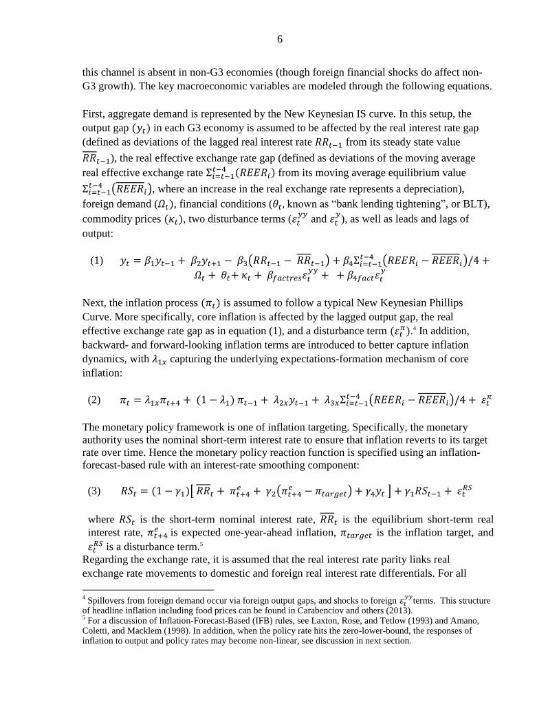
in equations (2) and in (A2) represent the effect of lagged output gap on

.

The EA4 GPM also features important nonlinearities such as the zero lower bound (ZLB)

on nominal interest rates, as well as the convex shape of the Phillips Curve discussed in

several other studies (e.g. IMF 2012).9 The idea is to better capture the current debate on

output gaps and the inflation/deflation spiral in the EA. The nonlinear Phillips curve is steep

or close to vertical when the output gap is largely positive. However, it flattens out when in

the case of a significant slack in the economy. In turn, this form of Phillips curve avoids

protracted deflationary spirals but it also enables having strong inflationary pressures when

the economy is above its productive capacities. The functional form is very similar to the

one used in Laxton et al (1995), Debelle et al (1997) and Laxton et al (1999). Without loss

8 See Appendix IV for the country-specific aggregate demand and inflation equations. In addition, gasoline and

consumer food prices are modeled in the same way as in GPM6. 9 The model also contains an option to non-linearize λ1 and λ3. The latter might be useful in some simulations to

enhance the flexibility of prices or price (real exchange rate) convergence within the union (for example in order to avoid large cyclicality in price dynamics).

9

of generality, the rest of the EA is modeled as a residual, in that its dynamics is calculated

after the model is solved for the EA block and the four large economies.

III. MODEL PROPERTIES, PARAMETERIZATION AND SIMULATION RESULTS

A. Parameterization and Model Fit

The calibration /estimation methodology for the parameters of the EA4 GPM is performed

to ensure that the model properties are sensible and broadly consistent with priors for the

EA economy and with historical data, thereby facilitating the interpretation of forecasts and

policy implications. This approach of calibration and Bayesian estimation falls between

fully micro-founded estimated DSGE models and pure time series models. Similar to

GPM6, a large proportion of the parameters are calibrated to account for county level

heterogeneity (Table 1).

As some of our important quarterly data series (in particular the Bank Lending Survey

data) used in the model start from the year 2003, the degrees of freedom in our estimation

are seriously limited. Only six parameters per large EA country were estimated (24 in total

while parameters of the rest of world are taken from GPM6) using Bayesian methods.

These are the elasticities with respect to real interest rates and real exchange rates in the

aggregate demand equation ( and ), the coefficients on the output gap ( ) and on the

real exchange rate ( ) in the Phillips-curve equation, and the short-term adjustment terms

in the gas and food price equations. The priors were chosen as the corresponding EA

parameters in GPM6. The estimation results (Table 1), reveal important differences

between country-level and EA-wide parameters. Parameters were generally not

significantly different from the priors; data were not too informative for identifying these

parameters. Germany’s and France’s output were estimated to be the most, while Italy and

Spain to be the least sensitive to real interest rate movements ( ). This might show that in

the latter two countries credit conditions were more affected by non-price related terms

than in the former two economies. Interestingly, the Phillips curves for core inflation in all

countries but France are estimated to be steeper ( ) than in the eurozone as a whole. This

can be the result of the fact that the rest of the countries in the eurozone are more open

economies, and in turn would have flatter Phillips curves. Unfortunately, the short sample

size did not allow us to test for possible structural changes in the parameters at the global

financial crisis.

A useful feature of the EA4 GPM is that it allows for intra-EA spillovers. The channels of

spillovers linking EA economies to the rest of EA and the world are specified through

spillover coefficients, which are calculated from the elasticities of trade and commodity

prices with respect to output in GPM6 10 (Table 2). Interestingly, for a given shock, the

biggest spillover to Germany comes from the rest of the world (RC6, including UK and

China) besides the rest of EA, implying strong economic linkages between Germany and

non-EA economies. In contrast, France, Italy, and Spain are more exposed to shocks

10

Appendix IV of Carabenciov and others (2013) provides detailed description on the calculation of the spillover coefficients.

10

generated within the Eurozone, and they all pass on significant spillovers to the rest of EA

(but less than Germany).

Table 1: Calibrated and estimated country-level parameters

Source: IMF staff estimations.

* The parameter was defined as a parameter for the Rest of the EA country group.

Source: IMF staff calculations

GR FR IT SP Eurozone

Distr mean se calibrated

beta3 gamma 0.10 0.20 0.13 0.10 0.07 0.06 0.10

beta4 gamma 0.07 0.20 0.08 0.11 0.05 0.09 0.07

lambda2x gamma 0.24 0.20 0.35 0.23 0.40 0.38 0.24

lambda3x gamma 0.15 0.20 0.12 0.12 0.13 0.10 0.15

iota_gas1 beta 0.14 0.10 0.27 0.17 0.32 0.24 0.14

iota_cfood1 beta 0.31 1.00 0.23 0.38 0.49 0.28 0.31

Calibrated parameters:

alpha1 … … … 0.72 0.72 0.72 0.72 0.72

alpha2 … … … 0.10 0.10 0.10 0.10 0.10

alpha3* … … … 0.10 0.10 0.10 0.10 0.10

alpha4* … … … 0.20 0.20 0.20 0.20 0.20

beta1 … … … 0.76 0.76 0.76 0.76 0.76

beta2 … … … 0.04 0.04 0.04 0.04 0.04

beta5 … … … -0.01 -0.01 -0.01 -0.01 -0.01

beta6 … … … 0.00 0.00 0.00 0.00 0.00

beta_fact … … … 0.55 0.55 0.55 0.55 0.55

beta_fact_res … … … 2.00 2.00 2.00 2.00 2.00

chi … … … … … … … 1.00

delta … … … … … … … 0.10

dot_lz_bar_ss_EU … … … … … … … 0.00

gamma1 … … … … … … … 0.69

gamma2 … … … … … … … 1.31

gamma4 … … … … … … … 0.20

iota_cfood2 … … … 0.03 0.03 0.03 0.03 0.03

iota_food3 … … … … … … … 0.10

iota_gas2 … … … 0.34 0.34 0.34 0.34 0.34

iota_oil3 … … … … … … … 0.10

kappa1* … … … 20.08 20.08 20.08 20.08 20.08

kappa2* … … … 0.00 0.00 0.00 0.00 0.00

lambda1x … … … 0.70 0.70 0.70 0.70 0.70

lambda4x … … … 0.05 0.05 0.05 0.05 0.05

phi … … … … … … … 0.83

tau … … … 0.20 0.20 0.20 0.20 0.20

theta … … … 0.30 0.30 0.30 0.30 0.30

Prior

Posterior mode

Estimated parameters:

11

Table 2: Spillover coefficients across countries and regions*

* The direct impacts of foreign demand shocks are the spillover coefficients multiplied by (calibrated at 2). For

more details see Appendix V. Source: IMF staff calculations.

B. Simulation results

When constructing a model for forecasting and policy analysis, one important consideration

is the response of the model to various shocks. This section presents the dynamic responses

to several types of shocks through impulse response functions and simulations, and describes

the major mechanisms that are at work in the model. The shocks analyzed can be grouped

into three types: (1) negative demand shocks emanating from either one (or all) major EA

country, or from outside the EA; (2) shocks leading to a deviation of the interest rate from the

monetary reaction function; (3) financial (BLT) shocks.11

Figure 3 shows that a negative one percentage point country specific demand shock

emanating from Germany feeds into lower demand in other economies immediately. As a

result, core inflation drops and the ECB lowers interest rates, accompanied by a gradual

depreciation of the euro. In turn, the depreciation of the currency makes the response of

headline inflation more muted (though in the scenario headline inflation declines more

quickly due to decline of oil price in the first few quarters).12

11

Only impulse responses around the non-stochastic steady state are presented in this section. Appendix II presents additional simulations starting from non-steady states with a case when policy rate is at the ZLB and the output gap is negative. 12

The reason is that the drop in crude oil prices due to lower global demand is partly offset by the depreciation of the euro, so that domestic gasoline and food prices do not fall as much as core inflation does.

from: GR FR IT SP Rest of EA US JA EA6 LA6 RC6

to:

GR … 0.04 0.03 0.02 0.09 0.03 0.01 0.03 0.01 0.09

FR 0.04 … 0.02 0.02 0.04 0.02 0.00 0.01 0.00 0.04

IT 0.03 0.03 … 0.02 0.03 0.02 0.00 0.01 0.00 0.04

SP 0.02 0.03 0.02 … 0.04 0.01 0.00 0.01 0.01 0.04

Rest of EA 0.12 0.06 0.03 0.02 … 0.04 0.01 0.02 0.00 0.10

EA 0.31 0.24 0.19 0.12 0.26 0.03 0.01 0.02 0.01 0.08

12

Figure 3: A negative demand shock in Germany

However, what happens in the source country of the shock, Germany, and in the other EA

countries is markedly different, largely due to a fixed nominal exchange rate. In a currency

union, the only way in which relative prices can adjust is through inflation (and ultimately

through real unit labor cost), but not through bilateral exchange rates. Therefore, a negative

demand shock in Germany would tend to depreciate the German real exchange rate, which

implies that inflation in Germany needs to fall faster than in other countries. As the ECB

only targets area-wide inflation and output, the cut in its policy rate would be less than

warranted if the Bundesbank were to react independently. As a result, German real interest

rates increase more than in other countries.

Figure 3 also shows that, as the shock starts to fade, the picture is reversed. German real

interest rates converge back to their steady state faster than in other countries, which adds an

additional boost to the German economy. As a result, both headline and core inflation in

Germany increase beyond their original steady state before finally converging back to their

steady state. Therefore, in the case of country specific demand shocks originating in member

countries of a currency union, price volatility and cyclicality in the source country is

amplified due to the absence of an exchange rate channel.

13

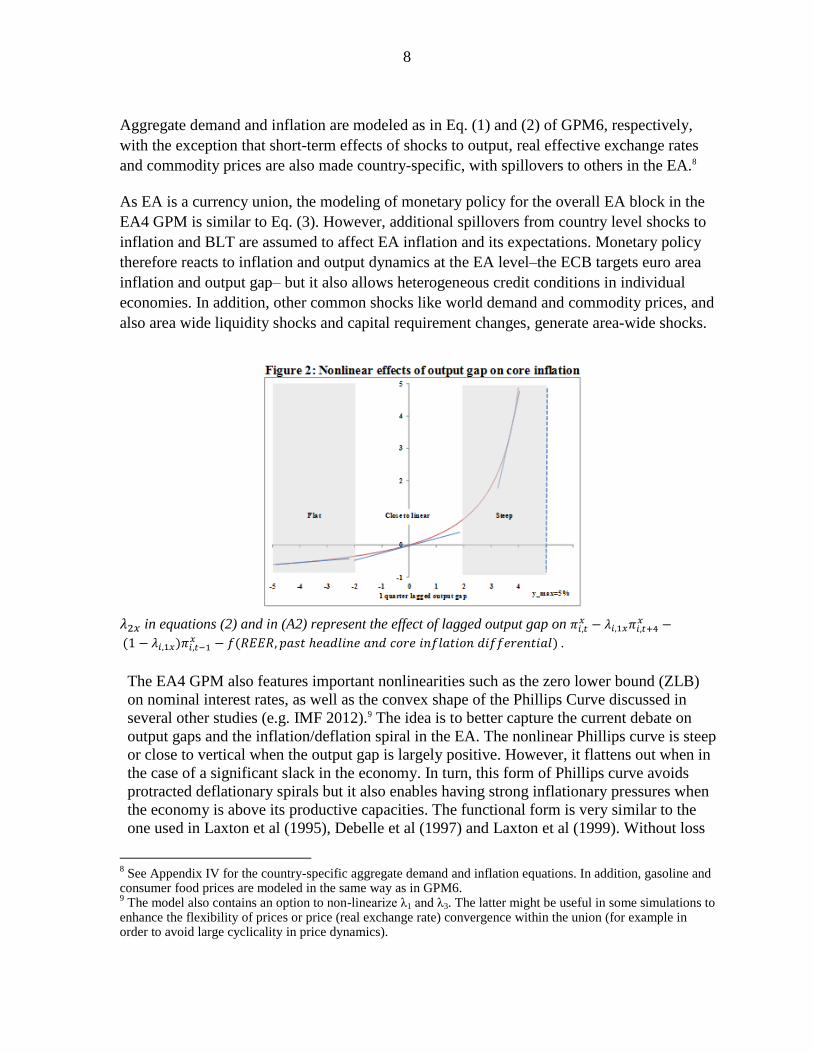
Figure 4: A common negative demand shock in the euro area

Figure 4 illustrates the role of the bilateral exchange rate when a common area-wide negative

demand shock hits the EA. In this case all countries are affected by the same negative

demand shock, and thus no significant bilateral real exchange rate adjustment is required

across euro area countries. In this case the cyclicality in prices disappears, the monetary

authority decreases area wide nominal interest rates, and real interest rates drop in all

countries. Although some differences occur between countries in the extent of price reactions

(and in turn in bilateral real exchange rates), these differences are smaller than with country

specific demand shocks. The initial drop in inflation gradually fades away in all countries.

14

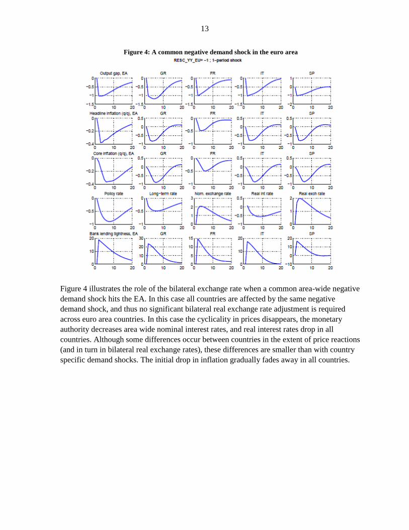
Figure 5: A euro area-wide interest rate shock

Figure 5 studies the effects of an exogenous departure from the interest rate reaction

function, specifically a transitory drop in the EA interest rate. The responses are as expected,

with the output gap rising in all countries as the real interest rate is temporarily reduced and

the real exchange rate is temporarily more depreciated than in steady state.

There are, however, country level differences. The boost to output is most significant for

Germany, but somewhat lower in Italy and Spain. There are two reasons: (1) Germany and

France have the largest estimated sensitivity of output to real interest rate changes; (2)

Despite Germany’s low estimated sensitivity of output to real exchange movements, its

output response is amplified by the spill-back from the rest of the world, given Germany’s

stronger connection with non-EA economies described in Section II.A. The same holds for

the response of core inflation, with Germany’s inflation most responsive to a monetary policy

shock.

15

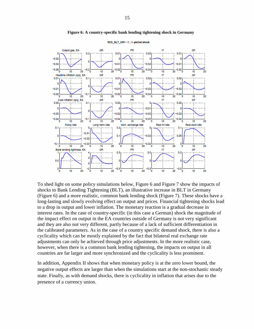
Figure 6: A country-specific bank lending tightening shock in Germany

To shed light on some policy simulations below, Figure 6 and Figure 7 show the impacts of

shocks to Bank Lending Tightening (BLT), an illustrative increase in BLT in Germany

(Figure 6) and a more realistic, common bank lending shock (Figure 7). These shocks have a

long-lasting and slowly evolving effect on output and prices. Financial tightening shocks lead

to a drop in output and lower inflation. The monetary reaction is a gradual decrease in

interest rates. In the case of country-specific (in this case a German) shock the magnitude of

the impact effect on output in the EA countries outside of Germany is not very significant

and they are also not very different, partly because of a lack of sufficient differentiation in

the calibrated parameters. As in the case of a country specific demand shock, there is also a

cyclicality which can be mostly explained by the fact that bilateral real exchange rate

adjustments can only be achieved through price adjustments. In the more realistic case,

however, when there is a common bank lending tightening, the impacts on output in all

countries are far larger and more synchronized and the cyclicality is less prominent.

In addition, Appendix II shows that when monetary policy is at the zero lower bound, the

negative output effects are larger than when the simulations start at the non-stochastic steady

state. Finally, as with demand shocks, there is cyclicality in inflation that arises due to the

presence of a currency union.

16

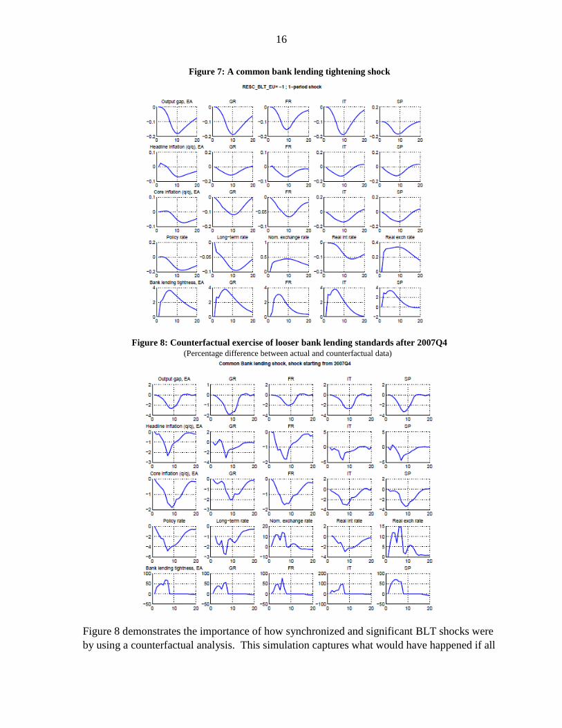
Figure 7: A common bank lending tightening shock

Figure 8: Counterfactual exercise of looser bank lending standards after 2007Q4

(Percentage difference between actual and counterfactual data)

Figure 8 demonstrates the importance of how synchronized and significant BLT shocks were

by using a counterfactual analysis. This simulation captures what would have happened if all

17

other estimated shocks had happened but not the BLT shocks such that the BLT level have

stayed constant at the level observed before the Great Financial Crisis. This simulation

highlights that a significant part (around 2 percent) of the euro area’s output drop during the

first wave of the Financial Crisis (2008-2009) can be attributed to tightening in credit

conditions. This negative ‘financial’ shock was more or less evenly distributed across

countries with the exception of Spain, which suffered disproportionately from the financial

shock. Inflation would have also been higher for a prolonged period of four about years.

Finally, Figure 9 shows that, on the other hand, the second financial shock in late 2011 and

early 2012 had a more diverse and more muted impact on the euro area as a whole and on

individual countries, in particular13 German and Spanish output were hardly affected by the

shock, while the output of France and Italy would have been reacting more strongly. Inflation

would also have been significantly higher (by about 0.5 percent) for two to three years after

the shock.

Figure 9: Counterfactual exercise of looser bank lending standards after 2011Q3

(Percentage difference between actual and counterfactual data)

13

The second counterfactual simulation shows what would have happened if BLT shocks were such that BLT remained flat after 2011Q3. In the case of Spain, the muted response of output in the second financial shock comes from a much negative loss in output during the first shock.

18

IV. FORECAST PERFORMANCE

One can measure the pure out-of-sample forecast performance properties of the model by the

Root Mean Squared Errors (RMSE). We compare the RMSE of EA4 GPM with GPM6 on

the EA block, and find that the model fit is similar. As there is no benchmark RMSE for the

four EA countries in GPM6, we present the RMSE over several in-sample forecast horizons

(one, four, and eight quarters) for the key variables (real GDP growth and inflation) in

Appendix Table A1. Overall, the forecast performance for real GDP growth at the EA level

is close to the one of GPM6, with some marginal improvement over the longer horizon. At

the country level, the model finds it more challenging to forecast Spain and Italy’s growth in

the short run, while at longer horizons the forecast performance improves markedly. On

inflation, the EA4 GPM underperforms GPM6 in the short run, but the difference is

diminishing over time. In sum, the more disaggregated model does not have worse longer-

term forecast performance than the more aggregated model at the eurozone level, while it

enables us to make forecasts at country level. Still, in a practical forecast exercise the

model’s performance can be significantly improved by adding additional information.

Next we turn our attention on how to incorporate additional information to the forecasts. To

do so, we show an illustrative forecasting exercise based on the EA4 GPM that was carried

out in 2014 Q2. The July 2012 WEO projection was partially based on this model run, but

obviously this run only served as one input among many others to the final projection.

For forecasting purposes global economic conditions are imported from GPM6 and treated as

exogenous. As a starting point of the forecast, “nowcasting” methods are used. These

forecasts make use of high frequency indictors such as country level industrial production

and PMIs. This improves the quality of the forecast, by linking it directly to the latest

economic indicators, and by

making it consistent with country-

level developments.

Developments in EA up to 2014

Q1 were mixed. Q1 growth in

Germany and Spain overshot the

April 2014 WEO forecast, while

France, Italy and several other EA

economies including the

Netherlands underperformed.

Inflation dipped to new lows well

below expectations, reflecting in

part continued slack in aggregate

demand across the region. Bank

lending and credit growth in the

EA remained weak, owing to

Table 3A. Selected Euro Area Countries: Growth Forecasts, 2014-16

WEO April 2014

2014 2015 2014 2015

Germany 1.7 1.6 2.1 1.8

France 1.0 1.5 0.7 1.3

Italy 0.6 1.1 0.2 1.3

Spain 0.9 1.0 1.0 1.2

Euro Area 1.2 1.5 1.0 1.6

Table3B. Selected Euro Area Countries: Inflation (Headline), 2014-16

(Percent, period average, yoy)

2014 2015 2014 2015

Germany 1.4 1.4 1.2 1.4

France 1.0 1.2 1.0 1.1

Italy 0.7 1.0 0.6 0.9

Spain 0.3 0.8 0.2 0.7

Euro Area 0.9 1.2 0.6 1.1

Sources: World Economic Outlook database; and staff simulations.

EA4 GPM June 2014

EA4 GPM June 2014WEO April 2014

19

continued deleveraging pressures and fragmentation.

During the same period, there was also some divergence in leading and high frequency

indicators across countries: PMIs in several EA economies softened slightly, orders in

Germany disappointed, but at the same time economic sentiments in EA remained relatively

optimistic. Given continued downward pressure in inflation, the ECB was expected to take a

policy action at its Governing Council meeting in early June, so that a policy rate cut of 10 to

15 basis points was assumed in the forecast. In addition, the fiscal stance of the four large EA

economies and of the EA overall was assumed to remain broadly unchanged from the

previous forecasting round.

Tables 3A and 3B and Appendix Figure 8 show the updated EA4 GPM forecast. Taking into

account all euro area developments, together with updated global economic conditions

imported from GPM6, the forecast suggests a slightly weaker EA outlook in 2014 compared

to the IMF’s April 2014 WEO. 2014 growth rates were revised down markedly in France

(from 1.0 to 0.7 percent) and Italy (from 0.6 to 0.2 percent), while being offset somewhat by

higher growth in Germany and Spain. As a result, the euro area was projected to grow at 1.0

percent in 2014, slightly below the April 2014 WEO forecast of 1.2 percent. Inflation was

expected to edge down further, to 0.6 percent in 2014 compared to 0.9 percent in the April

2014 WEO forecast, before picking up modestly in the following year.

V. CONCLUSIONS

The GPM project is designed to improve the toolkit for studying both own-country and cross-

country linkages. In this paper introduces a special version of GPM that includes the four

largest EA countries. The four economies Germany, France, Italy and Spain account for a

very significant share of euro area output. Breaking the single EA block of GPM6 into five

blocks, namely these four economies and the remaining economies of the EA, is therefore an

important enhancement to the existing framework that captures intra-EA dynamics in much

richer detail, including intra-EA spillovers, and also including the critical role of the single

currency and therefore of a common monetary policy.

As illustrated in the previous sections, the EA countries are more vulnerable to domestic and

external demand shocks because adjustments in the real exchange rate between EA countries

occur more gradually through inflation differentials. Spillovers from tight credit conditions in

each EA country are limited by direct trade channels and small confidence spillovers, but we

also consider scenarios where banks in all EU countries tighten credit conditions

simultaneously. In addition, the inclusion of more country-level information makes the

forecasting framework more robust, and consistent with individual country-level forecasts

carried out at the IMF. The approach taken accommodates differences between countries

through different parameterizations of a small number of equations, including spillover

coefficients.

20

Our preferred parameterization of the model replicates many of the key features of the EA

block in GPM6. For example, impulse response functions show the fundamentally different

behavior of country-level inflation when bilateral nominal exchange rates cannot adjust in the

face of idiosyncratic shocks, due to the presence of a currency union. The resulting cyclical

price effects are likely to be amplified in the case of country-specific shocks, owing to the

assumed reaction function of the European Central Bank, which is based on the aggregate

EA-level price level and EA-level output. Monetary policy in EA4 GPM uses conventional

inflation-forecast-based monetary reaction functions, as in other blocks of the model, while

non-conventional monetary policies, for example targeted LTROs, can be represented as EA-

wide or country-level shocks to bank lending conditions.

Future research in this area will focus on constructing a version of EA4 GPM that

incorporates other ongoing research work on GPM6, including a better integration of high

frequency indicators in the forecast, as well as a further decomposition of the current

emerging Asia and RC6 blocks by splitting out China and other large G20 economies. Given

the increasing economic linkages between the EA and emerging market economies, this

development will allow for a more comprehensive analysis of interactions among these

economies (see Blagrave and others, 2013).

21

References

Amano, R., D. Coletti, and T. Macklem, 1998, “Monetary Rules When Economic Behavior

Changes”, in: Monetary Policy Under Uncertainty: Papers from a Reserve Bank of

New Zealand Workshop, June 29–30, 1998.

Bailliu, J. and P. Blagrave, 2010, “The Transmission of Shocks to the Chinese Economy in a

Global Context: A Model-Based Approach”, Bank of Canada Working Paper, No.

2010–17.

Blagrave, P., P. Elliott, R. Garcia-Saltos, D. Hostland, D. Laxton and F. Zhang, 2013,

“Adding China to the Global Projection Model”, IMF Working Papers, WP/13/256.

Carabenciov, I., C. Freedman, R. Garcia-Saltos, O. Kamenik, D. Laxton, and P. Manchev,

2013, “GPM6—The Global Projection Model with 6 Regions”, IMF Working Papers,

WP/13/87.

Debelle, G. and D. Laxton, 1997, “Is the Phillips Curve Really a Curve? Some Evidence for

Canada, The United Kingdom and the United States,” IMF Staff Papers, Vol. 44, No.

2, June, pp. 249–82.

IMF, 2012, “World Economic Outlook: Coping with High Debt and Sluggish Growth”,

International Monetary Fund, Washington D.C.

IMF, 2014, “World Economic Outlook Update: An Uneven Global Recovery Continues”,

International Monetary Fund, Washington D.C.

Laxton, D., D. Rose and R. Tetlow, 1993, “Monetary Policy, Uncertainty and the

Presumption of Linearity”, Bank of Canada Technical Report, No. 63.

Laxton, D., G. Meredith and D. Rose, 1995, “Asymmetric Effects of Economic Activity on

Inflation: Evidence and Policy Implications,” IMF Staff Papers, Vol. 42, June,

(Washington: International Monetary Fund).

Laxton, D., D. Rose and D. Tambakis, 1999, ” The U.S. Phillips Curve The Case for

Asymmetry,” Journal of Economic Dynamics and Control, Vol. 23, No. 9, pp. 1459–

85.

Matheson, T., 2011, “New Indicators for Tracking Growth in Real Time”, IMF Working

Papers, WP 11/43.

Stock, J. and M. Watson, 1991, “A Probability Model of the Coincident Economic

Indicators”, in: Leading Economic Indicators: New Approaches and Forecasting

Records, edited by K. Lahiri and G. Moore, Cambridge University Press.

22

Appendix I. Out-of-sample forecast performance (RMSEs)

Table A1. Root Mean Squared Errors

1Q ahead 2Q ahead 8Q ahead

EA (GPM6) 2.8 2.7 2.9

EA (EA4 GPM) 2.8 2.7 2.7

Germany 3.6 3.5 3.7

France 3.0 2.7 2.2

Italy 3.9 3.5 3.1

Spain 4.7 3.6 2.7

EA (GPM6) 1.3 1.1 1.2

EA (EA4 GPM) 1.7 1.6 1.4

Germany 1.4 1.4 1.5

France 1.7 1.7 1.5

Italy 2.0 2.1 2.0

Spain 2.3 2.8 3.1

Source: IMF stafff calculations.

Real GDP growth (q/q saar)

Headline inflatin (q/q saar)

23

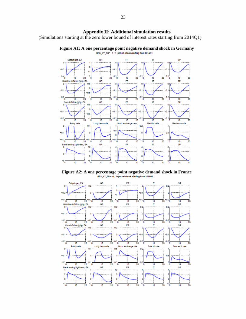
Appendix II: Additional simulation results

(Simulations starting at the zero lower bound of interest rates starting from 2014Q1)

Figure A1: A one percentage point negative demand shock in Germany

Figure A2: A one percentage point negative demand shock in France

24

Figure A3: A one percentage point negative demand shock in Italy

Figure A4: A one percentage point negative demand shock in Spain

25

Figure A5: A one percentage point common negative demand shock in the euro area

Figure A6: A country-specific bank lending tightening shock in Germany

26

Figure A7: A common bank lending tightening shock

Figure A8: A one percentage point negative demand shock in the US

27

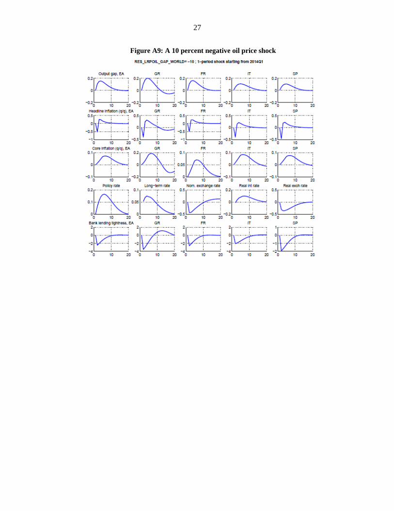
Figure A9: A 10 percent negative oil price shock

28

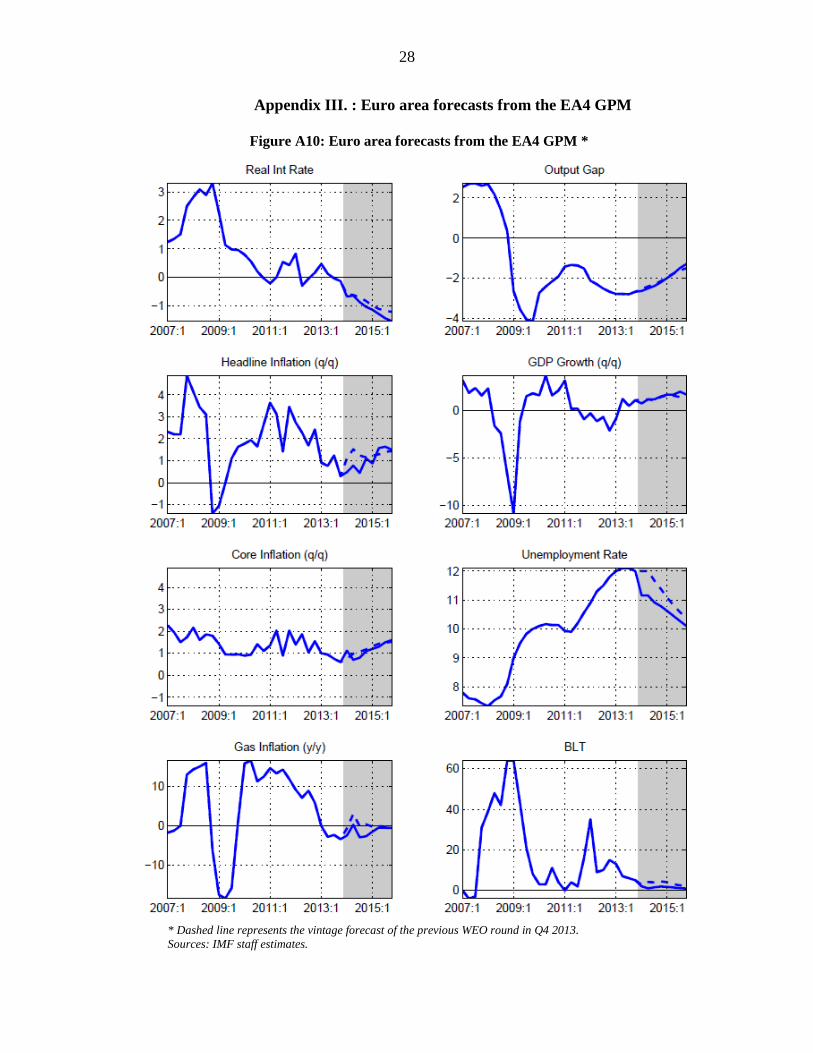
Appendix III. : Euro area forecasts from the EA4 GPM

Figure A10: Euro area forecasts from the EA4 GPM *

* Dashed line represents the vintage forecast of the previous WEO round in Q4 2013.

Sources: IMF staff estimates.

29

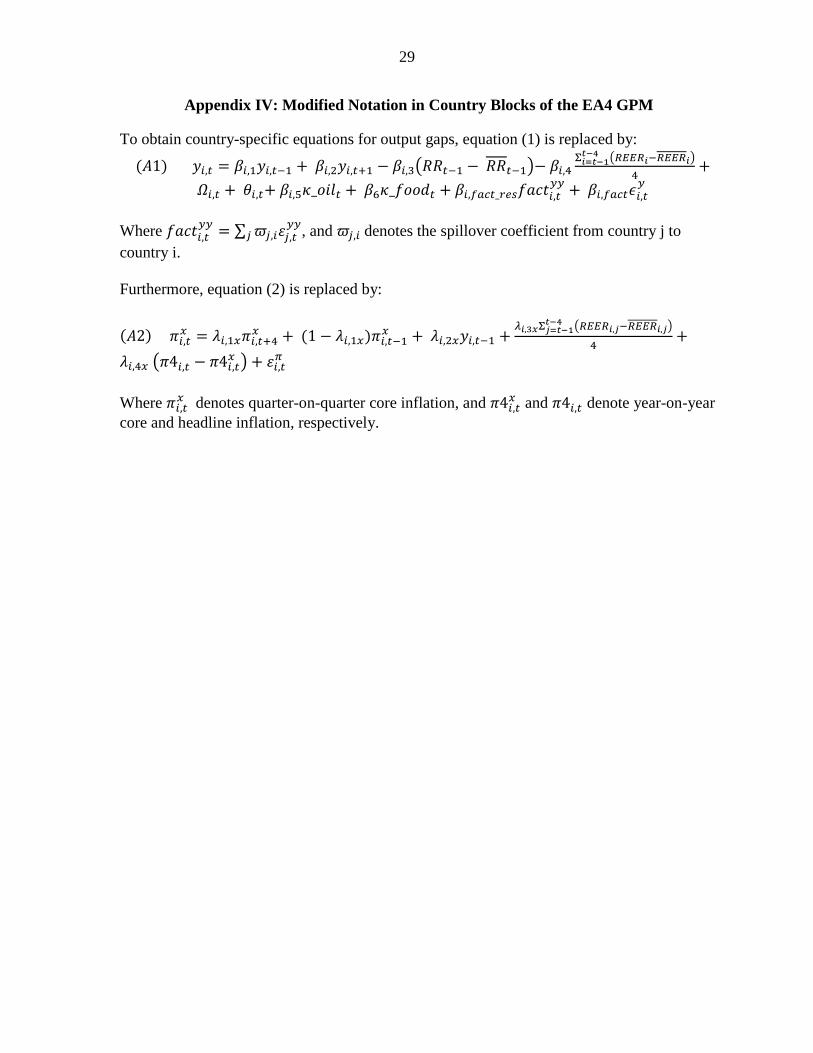
Appendix IV: Modified Notation in Country Blocks of the EA4 GPM

To obtain country-specific equations for output gaps, equation (1) is replaced by:

Where

, and denotes the spillover coefficient from country j to

country i.

Furthermore, equation (2) is replaced by:

Where denotes quarter-on-quarter core inflation, and

and denote year-on-year

core and headline inflation, respectively.

30

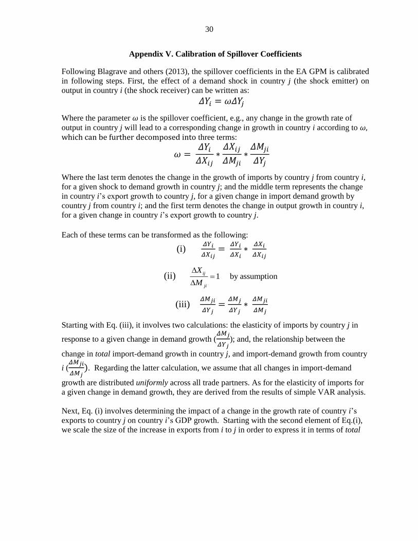
Appendix V. Calibration of Spillover Coefficients

Following Blagrave and others (2013), the spillover coefficients in the EA GPM is calibrated

in following steps. First, the effect of a demand shock in country j (the shock emitter) on

output in country i (the shock receiver) can be written as:

Where the parameter is the spillover coefficient, e.g., any change in the growth rate of

output in country j will lead to a corresponding change in growth in country i according to , which can be further decomposed into three terms:

Where the last term denotes the change in the growth of imports by country j from country i,

for a given shock to demand growth in country j; and the middle term represents the change

in country i’s export growth to country j, for a given change in import demand growth by

country j from country i; and the first term denotes the change in output growth in country i,

for a given change in country i’s export growth to country j.

Each of these terms can be transformed as the following:

(i)

(ii) 1 by assumptionij

ji

X

M

(iii)

Starting with Eq. (iii), it involves two calculations: the elasticity of imports by country j in

response to a given change in demand growth (

); and, the relationship between the

change in total import-demand growth in country j, and import-demand growth from country

i (

. Regarding the latter calculation, we assume that all changes in import-demand

growth are distributed uniformly across all trade partners. As for the elasticity of imports for

a given change in demand growth, they are derived from the results of simple VAR analysis.

Next, Eq. (i) involves determining the impact of a change in the growth rate of country i’s

exports to country j on country i’s GDP growth. Starting with the second element of Eq.(i),

we scale the size of the increase in exports from i to j in order to express it in terms of total

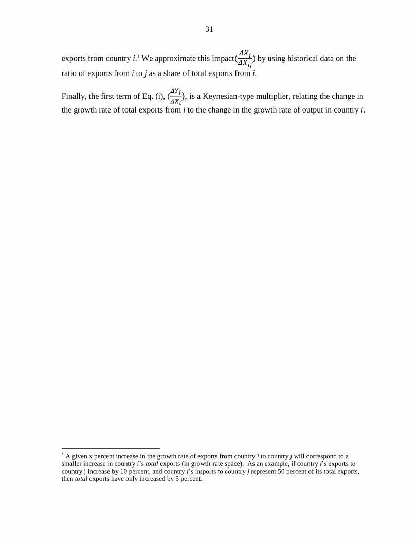
31

exports from country i.1 We approximate this impact

) by using historical data on the

ratio of exports from i to j as a share of total exports from i.

Finally, the first term of Eq. (i), (

), is a Keynesian-type multiplier, relating the change in

the growth rate of total exports from i to the change in the growth rate of output in country i.

1 A given x percent increase in the growth rate of exports from country i to country j will correspond to a

smaller increase in country i’s total exports (in growth-rate space). As an example, if country i’s exports to country j increase by 10 percent, and country i’s imports to country j represent 50 percent of its total exports, then total exports have only increased by 5 percent.