A Glimpse intoDiscrete Differential GeometryKeenan Crane, Max Wardetzky *

Communicated by Joel Hass

Note from Editor: The organizers of the 2018 JointMathematics Meetings Short Course on Discrete Dif-ferential Geometry have kindly agreed to providethis introduction to the subject. See p. XXX for moreinformation on the JMM 2018 Short Course.

The emerging field of discrete differential geometry(DDG) studies discrete analogues of smooth geometricobjects, providing an essential link between analyticaldescriptions and computation. In recent years it has un-earthed a rich variety of new perspectives on appliedproblems in computational anatomy/biology, computa-tional mechanics, industrial design, computational archi-tecture, and digital geometry processing at large. The ba-sic philosophy of discrete differential geometry is thata discrete object like a polyhedron is not merely an ap-proximation of a smooth one, but rather a differential ge-ometric object in its own right. In contrast to traditionalnumerical analysis which focuses on eliminating approx-imation error in the limit of refinement (e.g., by takingsmaller and smaller finite differences), DDG places anemphasis on the so-called “mimetic” viewpoint, wherekey properties of a system are preserved exactly, inde-pendent of how large or small the elements of a meshmight be. Just as algorithms for simulating mechani-cal systems might seek to exactly preserve physical in-variants such as total energy or momentum, structure-preserving models of discrete geometry seek to exactlypreserve global geometric invariants such as total curva-ture. More broadly, DDG focuses on the discretization ofobjects that do not naturally fall under the umbrella oftraditional numerical analysis. This article provides anoverview of some of the themes in DDG.

The Game. Our article is organized around a “game” of-ten played in discrete differential geometry in order tocome up with a discrete analogue of a given smooth ob-ject or theory:

1. Write down several equivalent definitions in thesmooth setting.

2. Apply each smooth definition to an object in the dis-crete setting.

3. Analyze trade-offs among the resulting discrete def-initions, which are invariably inequivalent.

*Keenan Crane is assistant professor of computer science at CarnegieMellon University. His e-mail address is kmcrane@cs.cmu.edu.Max Wardetzky is professor of mathematics at University of Göttin-gen. His e-mail address is wardetzky@math.uni-goettingen.de.

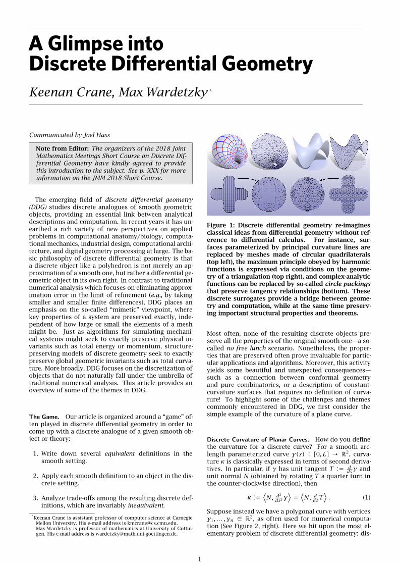
Figure 1: Discrete differential geometry re-imaginesclassical ideas from differential geometry without ref-erence to differential calculus. For instance, sur-faces parameterized by principal curvature lines arereplaced by meshes made of circular quadrilaterals(top left), the maximum principle obeyed by harmonicfunctions is expressed via conditions on the geome-try of a triangulation (top right), and complex-analyticfunctions can be replaced by so-called circle packingsthat preserve tangency relationships (bottom). Thesediscrete surrogates provide a bridge between geome-try and computation, while at the same time preserv-ing important structural properties and theorems.

Most often, none of the resulting discrete objects pre-serve all the properties of the original smooth one—a so-called no free lunch scenario. Nonetheless, the proper-ties that are preserved often prove invaluable for partic-ular applications and algorithms. Moreover, this activityyields some beautiful and unexpected consequences—such as a connection between conformal geometryand pure combinatorics, or a description of constant-curvature surfaces that requires no definition of curva-ture! To highlight some of the challenges and themescommonly encountered in DDG, we first consider thesimple example of the curvature of a plane curve.

Discrete Curvature of Planar Curves. How do you definethe curvature for a discrete curve? For a smooth arc-length parameterized curve 𝛾(𝑠) ∶ [0, 𝐿] → ℝ2, curva-ture 𝜅 is classically expressed in terms of second deriva-tives. In particular, if 𝛾 has unit tangent 𝑇 ∶= 𝑑

𝑑𝑠𝛾 andunit normal 𝑁 (obtained by rotating 𝑇 a quarter turn inthe counter-clockwise direction), then

𝜅 ∶= ⟨𝑁, 𝑑2

𝑑𝑠2 𝛾⟩ = ⟨𝑁, 𝑑𝑑𝑠𝑇⟩ . (1)

Suppose instead we have a polygonal curve with vertices𝛾1,… ,𝛾𝑛 ∈ ℝ2, as often used for numerical computa-tion (See Figure 2, right). Here we hit upon the most el-ementary problem of discrete differential geometry: dis-

1

crete geometric objects are often not sufficiently differ-entiable (in the classical sense) for standard definitionsto apply. For instance, our curvature definition (Equa-tion 1) causes trouble, since at vertices our discrete curveis not twice differentiable, nor does it have well definednormals. The basic approach of DDG is to find alterna-tive characterizations in the smooth setting that can beapplied to discrete geometry in a natural way. With cur-vature, for instance, we can apply the fundamental theo-rem of calculus to Equation 1 to acquire a different state-ment: if 𝜑 is the angle from the horizontal to 𝑇, then

∫𝑏

𝑎𝜅 𝑑𝑠 = 𝜑(𝑏) −𝜑(𝑎) mod 2𝜋.

Put more simply: curvature is the rate at which the tan-gent turns. This characterization can be applied natu-rally to our polygonal curve: along any edge the changein angle is clearly zero. At a vertex it is simply the turn-ing angle 𝜃𝑖 ∶= 𝜑𝑖,𝑖+1 − 𝜑𝑖−1,𝑖 between the directions𝜑𝑖−1,𝑖,𝜑𝑖,𝑖+1 of the two incident edges, yielding our firstnotion of discrete curvature:

𝜅𝐴𝑖 ∶= 𝜃𝑖 ∈ (−𝜋,𝜋). (2)

Are there other characterizations that also lead natu-rally to a discrete formulation? Yes: for instance wecan consider the motion of 𝛾 that most quickly reducesits length. In the smooth case it is well known thatthe change in length with respect to a smooth variation𝜂(𝑠) ∶ [0, 𝐿] → ℝ2 that vanishes at endpoints is given byintegration against curvature:

𝑑𝑑𝜀|𝜀=0

length(𝛾 + 𝜀𝜂) = −∫𝐿

0⟨𝜂(𝑠), 𝜅(𝑠)𝑁(𝑠)⟩ 𝑑𝑠.

Hence, the velocity that most quickly reduces length is𝜅𝑁. For a polygonal curve, we can simply differentiatethe sum of the edge lengths 𝐿 ∶= ∑𝑛−1

𝑖=1 |𝛾𝑖+1 − 𝛾𝑖| withrespect to any vertex position. At a vertex 𝑖 we obtain

𝜕𝛾𝑖𝐿 = 𝛾𝑖 −𝛾𝑖−1|𝛾𝑖 −𝛾𝑖−1|

− 𝛾𝑖+1 −𝛾𝑖|𝛾𝑖+1 −𝛾𝑖|

=∶ 𝑇𝑖−1,𝑖 −𝑇𝑖,𝑖+1, (3)

i.e., just a difference of unit tangent vectors 𝑇𝑖,𝑖+1 alongconsecutive edges. If 𝑁𝑖 ∈ ℝ2 is the unit angle bisectorat vertex 𝑖, this difference can also be expressed as

𝜅𝐵𝑖 𝑁𝑖 ∶= 2 sin(𝜃𝑖/2)𝑁𝑖, (4)

providing a discretization of the curvature normal 𝜅𝑁.A closely-related idea is to consider how the length ofa curve changes if we displace it by a small constantamount in the normal direction. As observed by Steiner,the new length can be expressed as

length(𝛾 + 𝜀𝑁) = length(𝛾) − 𝜀∫𝐿

0𝜅(𝑠) 𝑑𝑠. (5)

Since this formula holds for any small piece of thecurve, it can be used to obtain a notion of curvature ateach point. How dowe define normal offsets in the polyg-onal case? At vertices we again encounter the issue thatwe have no notion of normals. One idea is to break thecurve into individual edges which can then be translatedby 𝜀 along their respective normal directions. We canthen close the gaps between edges in a variety of ways:using (A) a circular arc of radius 𝜀, (B) a straight line, or by(C) extending the edges until they intersect (see Figure 3).If we then calculate the lengths for these new curves, weget

length𝐴 = length(𝛾) − 𝜀∑𝑛−1𝑖=2 𝜃𝑖,

length𝐵 = length(𝛾) − 𝜀∑𝑛−1𝑖=2 2 sin(𝜃𝑖/2),

length𝐶 = length(𝛾) − 𝜀∑𝑛−1𝑖=2 2 tan(𝜃𝑖/2).

Figure 2: A given geometric quantity from the smoothsetting, like curvature 𝜅, may have several reasonabledefinitions in the discrete setting. Discrete differentialgeometry seeks definitions that exactly replicate prop-erties of their smooth counterparts.

Mirroring the observation in the smooth setting, we cannow say that whatever change we observe in the lengthprovides a definition for discrete curvature. The first twoare the same as ones we have seen already: the circu-lar arc yielding the expression from Equation 2, and thestraight line corresponding to Equation 4. The third oneprovides yet another notion of discrete curvature

𝜅𝐶𝑖 ∶= 2 tan(𝜃𝑖/2).

Finally, in the smooth case it is also well known that cur-vature has magnitude equal to the inverse of the radiusof the so-called osculating circle, which agrees with thecurve up to second order. A natural way to define anosculating circle for a polygon is to take the circle pass-ing through a vertex and its two neighbors. From theformula for the radius 𝑅𝑖 of a circumcircle in terms ofthe side lengths of the corresponding triangle, one eas-ily gets a discrete curvature that is different from the onewe saw before:

𝜅𝐷𝑖 ∶= 1/𝑅𝑖 = 2 sin(𝜃𝑖)/𝑤𝑖, (6)

where 𝑤𝑖 ∶= |𝛾𝑖+1 − 𝛾𝑖−1|. Apart from merely beingdifferent expressions, we can notice that 𝜅𝐴, 𝜅𝐵 and 𝜅𝐶

are all invariant under a uniform scaling of the curve,whereas 𝜅𝐷 scales like the smooth curvature 𝜅. This sit-uation demonstrates another common phenomenon indiscrete differential geometry, namely that dependingon which smooth characterization is used as a startingpoint, onemay end up with pointwise or integrated quan-tities in the discrete case.

Figure 3: Different characterizations of curvature inthe smooth setting naturally lead to different notionsof discrete curvature. (Here we abbreviate 𝑇𝑖,𝑖+1 and𝑇𝑖−1,𝑖 by 𝑢 and 𝑣, respectively.)

2

Figure 4: Typically, not all properties of a smooth ob-ject can be preserved exactly at the discrete level. Forcurve-shortening flow, for example, 𝜅𝐴 exactly pre-serves the total curvature, 𝜅𝐵 exactly preserves thecenter of mass, and with 𝜅𝐶 the flow remains station-ary (up to rescaling) for any circular solution. How-ever, no local definition of discrete curvature can pro-vide all three properties simultaneously.

As one might imagine, there are many other possiblestarting points for obtaining a discrete analogue of cur-vature. Eventually, however, all starting points end upleading back to the same definitions, suggesting thatthere may be only so many possibilities. For example,if 𝜙 ∶ ℝ2 → ℝ is the signed distance from a smoothclosed curve 𝛾, then applying the Laplacian Δ yields thecurvature of its level curves; in particular, Δ𝜙|𝜙=0 yieldsthe curvature of 𝛾. Likewise, if we apply the Laplacianto the signed distance function for a discrete curve, werecover 𝜅𝐴 on one side and 𝜅𝐵 on the other. Yet anotherapproach is the theory of normal cycles (as discussed byMorvan), related to the Steiner formula from Equation (5).Here, rather than settle on a single normal𝑁𝑖 at each ver-tex we consider all unit vectors between the unit normalsof the two incident edges, ultimately leading back to thefirst discrete curvature 𝜅𝐴. This theory applies equallywell to both smooth and polygonal curves, again rein-forcing the perspective that the fundamental behavior ofgeometry is neither inherently smooth nor discrete, butcan be well captured in both settings by picking the ap-propriate ansatz. More broadly, the fact that equivalentcharacterizations in the smooth setting lead to differentinequivalent definitions in the discrete setting is not spe-cial to the case of curves, but is one of the central themesin discrete differential geometry.

From here, a natural question arises: which discretecurvature is “best”? A traditional criterion for discrimi-nating among different discrete versions is the questionof convergence: if we consider finer and finer approx-imating polygons, will our discrete curvatures convergeto the classical smooth one? However, convergence doesnot always single out a best version: treated appropri-ately, all four of our discrete curvatures will converge.We must therefore look beyond convergence, toward ex-act preservation of properties and relationships from thesmooth setting. Which properties should we try to pre-serve? The answer of course depends on what we aim touse these curvatures for.

As a toy example, consider the curve-shortening flow(depicted in Figure 4, top left), where a curve evolvesaccording to the velocity that most quickly reduces itslength. As discussed above, this velocity is equal to the

curvature normal 𝜅𝑁. A smooth, simple curve evolvingunder this flow exhibits several basic properties: it hasat all times total curvature 2𝜋, its center of mass re-mains fixed, it tends toward a circle of vanishing radius,and remains embedded for all time, i.e., no self-crossingsarise (Gage-Grayson-Hamilton). Do our discrete curva-tures furnish these same properties? A numerical exper-iment is shown in Figure 4. Here we evolve our polygonby a simple time-discrete flow 𝛾𝑖 ← 𝛾𝑖 + 𝜏𝜅𝑖𝑁𝑖 with afixed time step 𝜏 > 0. For 𝜅𝐷, 𝑁𝑖 is the unit vector alongthe circumradius; otherwise it is the unit angle bisector.Not surprisingly, 𝜅𝐴 preserves total curvature (due tothe fundamental theorem of calculus); 𝜅𝐵 does not drift(consider summing Equation 3 over all vertices); and 𝜅𝐷

has circular polygons as limit points (since all velocitiespoint toward the center of a common circle). However,no discrete curvature satisfies all three properties simul-taneously. Moreover, for a constant time step 𝜏 no suchflow can guarantee that new crossings do not occur. Thissituation illustrates the no free lunch idea: no matterhow hard we try, we cannot find a single discrete objectthat preserves all the properties of its smooth counter-part. Instead, we have to pick and choose the propertiesbest suited to the task at hand.

Suppose that instead of curvature flow, we considertwo other beautiful topics in the geometry of planecurves: the Whitney–Graustein theorem, which classifiesregular homotopy classes of curves by their total curva-ture, and Kirchhoff’s famous analogy between motionsof a spherical pendulum and elastic curves, i.e., curvesthat extremize the bending energy ∫𝐿0 𝜅2 𝑑𝑠 subject toboundary conditions. Among the curvatures discussedabove, only 𝜅𝐴 provides a discrete version of Whitney–Graustein, but does not provide an exact discrete ana-logue of Kirchhoff. Likewise, 𝜅𝐶 preserves the struc-ture of the Kirchhoff analogy, but notWhitney–Graustein.This kind of no free lunch situation is a characteristic fea-ture of DDG. A similar obstacle is encountered in the the-ory of ordinary differential equations, where it is knownthat there are no numerical integrators for Hamiltoniansystems that simultaneously conserve energy, momen-tum, and the symplectic form. From a computationalpoint of view, making judicious choices about whichquantities to preserve for which applications goes hand-in-hand with providing formal guarantees on the reliabil-ity and robustness of algorithms.

We now give a few glimpses into recent topics andtrends in DDG.

Discrete Conformal Geometry A conformal map is,roughly speaking, a map that preserves angles (see Fig-ure 1, bottom left). A good example is Mercator’s pro-jection of the globe: even though area gets stretchedout badly—making Greenland look much bigger thanAustralia!—the directions “north” and “east” remain atright angles, which is very helpful if you’re trying to nav-igate the sea. A beautiful fact about conformal mapsis that any surface can be conformally mapped to aspace of constant curvature (“uniformization”), provid-ing it with a canonical geometry. This fact, plus thefact that conformal maps can be efficiently computed(e.g., by solving sparse linear systems), have led in recentyears to widespread development of conformal mappingalgorithms as a basic building block for digital geometryprocessing algorithms. In applications, discrete confor-mal maps are used for everything from sensor network

3

Figure 5: What is the simplicial analogue of a confor-mal map? Requiring all angles to be preserved is toorigid, forcing a global similarity (left). Asking only forpreservation of so-called length cross ratios providesjust the right amount of flexibility, maintaining muchof the structure found in the smooth setting such asinvariance under Möbius transformations (right)

layout to comparative analysis of medical or anatomicaldata. Of course, to process real data one must be able tocompute conformal maps on discrete geometry.

What does it mean for a discrete map to be conformal?As with curvature, one can play the game of enumerat-ing several equivalent characterizations in the smoothsetting. Consider for instance a map 𝑓 ∶ 𝑀 → 𝐷2 ⊂ ℂfrom a disk-like surface 𝑀 with Riemannian metric 𝑔 tothe unit disk 𝐷2 in the complex plane. This map is con-formal if it preserves angles, if it preserves infinitesimalcircles, if it can be expressed as a pair of real conjugateharmonic functions 𝑓 = 𝑎+𝑏𝑖, if it is a critical point ofthe Dirichlet energy ∫𝑀 |𝑑𝑓|2 𝑑𝐴, or if it induces a newmetric ̃𝑔 ∶= 𝑑𝑓 ⊗ 𝑑𝑓 that at each point is a positiverescaling of the original one: ̃𝑔 = 𝑒2𝑢𝑔. Each startingpoint leads down a path toward different consequencesin the discrete setting, and to algorithms with differentcomputational tradeoffs.

Oddly enough, the most elementary characterizationof conformal maps, angle preservation, does not trans-late very well to the discrete setting (see Figure 5). Con-sider for instance a simplicial map that takes a triangu-lated disk 𝐾 = (𝑉,𝐸,𝐹) to a triangulation in the plane.Any map that preserves interior angles will be a similar-ity on each triangle, i.e., it can only rigidly rotate andscale. But since adjacent triangles share edges, the scalefactor for all triangles must be identical. Hence, the onlydiscrete surfaces that can be conformally flattened inthis sense are those that are (up to global scale) devel-opable, i.e., that can be rigidly unfolded into the plane.This outcome is in stark contrast to the smooth setting,where any disk can be conformally flattened. This sit-uation reflects a common scenario in DDG: rigidity, orwhat in finite element analysis is sometimes called lock-ing. There are simply too few degrees of freedom relativeto the number of constraints: we want to match anglesat all 3𝐹 corners, but have only 2𝑉 < 3𝐹 degrees of free-dom. Hence, if we insist on angle preservation we haveno chance of capturing the flexibility of smooth confor-mal maps.

Other characterizations provide greater flexibility.One idea is to associate each vertex of our discrete disk𝐾 with a circle in the plane. A theorem of Koebe impliesthat one can always arrange these circles such that twocircles are tangent if they belong to a shared edge and allboundary circles are tangent to a common circle bound-ing the rest. For a regular triangular lattice approximat-

ing a region 𝑈 ⊂ ℂ, Thurston noticed that this map ap-proximates a smooth conformal map 𝑓 ∶ 𝑈 → 𝐷2 as theregion is filled by smaller and smaller circles (see Fig-ure 1, bottom), as later proved by Rodin and Sullivan.Unlike a traditional finite element discretization, theseso-called circle packings also preserve many of the basicstructural properties of conformal maps. For instance,composition with a Möbius transformation of the diskyields another uniformization map, as in the smoothsetting. More broadly, circle packings provide an un-expected bridge between geometry and combinatorics,since the geometry of a map is determined entirely byincidence relationships 1. On the flip side, this means adifferent theory is needed to account for the geometryof irregular triangulations, as more commonly used inapplications.

An alternative theory starts from the idea that undera conformal map the Riemannian metric 𝑔 experiences auniform scaling at each point: ̃𝑔 = 𝑒2𝑢𝑔. In other words,vectors tangent to a given point 𝑝 ∈ 𝑀 shrink or grow bya positive factor 𝑒𝑢. In the simplicial setting𝑔 is replacedby a piecewise Euclidean metric, i.e., a collection of pos-itive edge lengths ℓ ∶ 𝐸 → ℝ>0 that satisfy the triangleinequality in each face. Two such metrics ℓ, ̃ℓ are thensaid to be discretely conformally equivalent if they are re-lated by ̃ℓ𝑖𝑗 = 𝑒(𝑢𝑖+𝑢𝑗)/2ℓ𝑖𝑗 for any collection of discretescale factors 𝑢 ∶ 𝑉 → ℝ. Though at first glance this re-lationship looks like a simple numerical approximation,it turns out to provide a complete discrete theory thatpreserves much of the structure found in the smoothsetting, with close ties to theories based on circles. Anequivalent characterization is the preservation of lengthcross ratios 𝔠𝑖𝑗𝑘𝑙 ∶= ℓ𝑖𝑗ℓ𝑘𝑙/ℓ𝑗𝑘ℓ𝑙𝑖 associated with eachedge 𝑖𝑗 ∈ 𝐸; for a mesh embedded in ℝ𝑛 these ratiosare invariant under Möbius transformations, again mim-icking the smooth theory. This theory also leads to effi-cient, convex algorithms for discrete Ricci flow, which isa starting point for many applications in digital geome-try processing.

More broadly, discrete conformal geometry and dis-crete complex analysis is an active area of research, withelegant theories not only for triangulations but also forlattice-based discretizations, which make contact withthe topic of (discrete) integrable systems, discussed be-low. Yet basic questions about properties like conver-gence, or descriptions that are compatible with extrinsicgeometry, are still only starting to be understood.

Discrete Differential Operators Differential geometryand in particular Riemannian manifolds can be studiedfrom many different perspectives. In contrast to thepurely geometric perspective (based on, say, notions ofdistance or curvature), differential operators provide avery different point of view. One of the most funda-mental operators in both physics and geometry is theLaplace–Beltrami operator Δ (or Laplacian for short) act-ing on differential 𝑘-forms. It describes, for example,heat diffusion, wave propagation, steady state fluid flow,and is key to the Schrödinger equation in quantum me-chanics. It also provides a link between analytical andtopological information: for instance, on closed Rieman-nian manifolds the dimension of harmonic 𝑘-forms (i.e.,those in the kernel of Δ) equals the dimension of the1See “Circle Packing” in the December 2003 Notices

http://www.ams.org/notices/200311/fea-stephenson.pdf

4

𝑘th cohomology—a purely topological property. Thespectrum of the Laplacian (i.e., the list of eigenvalues)likewise reveals a great deal about the geometry of themanifold. For example, the first nonzero eigenvalueof the 0-form Laplacian provides an upper and a lowerbound on optimally cutting a compact Riemannian man-ifold 𝑀 into two disjoint pieces of, loosely speaking,maximal volume and minimal perimeter (Cheeger-Buser).These so-called Cheeger cuts have a wide range of ap-plications across machine learning and computer vision;more broadly, eigenvalues and eigenfunctions of Δ helpto generalize traditional Fourier-based simulation andsignal processing to more general manifolds.

These observations motivate the study of discreteLaplacians, which can be defined even in the purely com-binatorial setting of graphs. Here we briefly outline theirdefinition for orientable finite simplicial 𝑛-manifolds,such as polyhedral surfaces, without boundary. Our ex-position is similar to what has become known as discreteexterior calculus. To this end, consider the simplicialboundary operators 𝜕𝑘 ∶ 𝐶𝑘 → 𝐶𝑘−1 acting on 𝑘-chains(i.e., formal linear combinations of 𝑘-simplices). The cor-responding dual spaces (cochains) 𝐶𝑘 ∶= Hom(𝐶𝑘, ℝ)and respective dual operators 𝛿𝑘 ∶ 𝐶𝑘 → 𝐶𝑘+1 give riseto the chain complex

{0} → 𝐶0 → 𝐶1 → … → 𝐶𝑛 → {0}.

The chain property says that 𝛿𝑘∘𝛿𝑘−1 = 0, and one henceobtains simplicial cohomology 𝐻𝑘 ∶= ker(𝛿𝑘)/im(𝛿𝑘−1).To define a Laplacian in this setting, we equip each 𝐶𝑘

with a positive definite inner product (⋅, ⋅)𝑘, and let 𝛿∗𝑘 be

the adjoint operator with respect to these inner products,i.e., (𝛿𝑘𝛼,𝛽)𝑘+1 = (𝛼,𝛿∗

𝑘𝛽)𝑘 for all 𝛼,𝛽. The Laplacianon 𝑘-cochains is then defined as

Δ𝑘 ∶= 𝛿∗𝑘𝛿𝑘 +𝛿𝑘−1𝛿∗

𝑘−1.

The resulting space of harmonic 𝑘-chains, {𝛼 ∈𝐶𝑘|Δ𝑘𝛼 = 0} is then isomorphic to 𝐻𝑘—just as in thesmooth setting. This fact is independent of the choiceof inner product, mirroring the fact that cohomology de-pends only on topological structure. Likewise, for anyinner product one obtains a discrete Hodge decomposi-tion

𝐶𝑘 = ker(Δ𝑘) ⊕ im(𝛿𝑘−1) ⊕ im(𝛿∗𝑘 ),

where here the subspaces do depend on the choice ofinner product.

At this point we return again to the game of DDG:which choice of inner product is best? A trivial dotproduct leads to purely combinatorial graph Laplacians,which do not (in general) converge to their smooth coun-terparts (e.g., when approximating a smooth manifoldby a polyhedral one). Another choice is to consider lin-ear interpolation of 𝑘-cochains over 𝑛-dimensional sim-plices, resulting in what are known as Whitney elements.For 𝑛 = 2, we get the so-called cotan Laplacian (Pinkalland Polthier), which is widely used in digital geometryprocessing. Though other choices are possible, we againencounter a no free lunch situation: no choice of innerproduct can preserve all the properties of the smoothLaplacian. Which properties do we care about? Be-yond convergence, perhaps the most desirable proper-ties are the maximum principle (which ensures, for in-stance, proper behavior for heat flow), and the propertythat, for flat domains, linear functions are in the ker-nel (leading to a proper definition of barycentric coor-dinates). For general unstructured meshes there are no

Figure 6: Left: two discrete parameterizations of apseudosphere (constant Gauß curvature 𝐾 = −1), onewith a Chebychev net along asymptotic directions (left)and another along principal curvature lines (right).Right: a discrete Chebyshev net on a surface of vary-ing curvature, resembling the weft and warp direc-tions of a woven material.

discrete Laplacians with all of these properties. How-ever, certain types of meshes (such as Delaunay triangu-lations) do indeed allow for “perfect” discrete Laplacians,offering a connection between geometry and (discrete)differential operators.

Discrete Integrable Systems Another topic that has pro-vided inspiration for many ideas in DDG is parameter-ized surface theory. Consider for instance the problemof dressing a given surface by a fishnet stocking, i.e., awoven material composed of inextensible yarns follow-ing transversal “warp” and “weft” directions (see Figure6, right). This task corresponds to decorating a surfacewith a tiling where each vertex is incident to four par-allelograms. Infinitesimally, such a tiling is known as aweak Chebyshev net (Chebyshev 1878), and locally corre-sponds to a regularly parameterized surface 𝑓 ∶ 𝑈 ⊂ℝ2 → ℝ3 where the directional derivatives 𝑓𝑢 and 𝑓𝑣along the coordinate directions satisfy |𝑓𝑢|𝑣 = |𝑓𝑣|𝑢 = 0,i.e., partial derivatives with respect to one parameterhave constant length along the parameter lines of theother parameter. The special case of rhombic tilings(|𝑓𝑢| = |𝑓𝑣| = 1) are known as (strong) Chebyshev nets.Can every smooth surface be wrapped in a stocking? Lo-cally (i.e., in a small patch around any given point) theanswer is “yes”. Globally, however, there are severe ob-structions to doing so, which provide some fascinatingconnections to physics.

Consider for instance the special case of so-called K-surfaces, characterized by constant Gauß curvature 𝐾 =−1. Every K-surface admits a parameterization 𝑓 ∶ 𝑈 ⊂ℝ2 → ℝ3 aligned with the two transversal asymptotic di-rections along which normal curvature vanishes. Hence,if 𝑁 is the unit surface normal then

⟨𝑓𝑢𝑢,𝑁⟩ = ⟨𝑓𝑣𝑣,𝑁⟩ = 0. (7)

Asymptotic parameterizations are weak Chebyshev netssince

𝑎 ∶= |𝑓𝑢|, 𝑏 ∶= |𝑓𝑣| satisfy 𝑎𝑣 = 𝑏𝑢 = 0. (8)

Moreover, one can show that the angle𝜙 between asymp-totic lines satisfies the sine-Gordon equation

𝜙𝑢𝑣 −𝑎𝑏 sin𝜙 = 0, (9)

and conversely, every solution to the sine-Gordon equa-tion describes a parameterized K-surface. Hilbert usedthis equation (and Chebyshev nets) to prove that the

5

Figure 7: Discrete parameterized surfaces play a role inarchitectural geometry, where special incidence rela-tionships on quadrilaterals translate to manufacturingconstraints like zero nodal torsion, or offset surfacesof constant thickness. Here a curvature line parame-terized surface discretized by a conical net is used inthe design of a railway station (courtesy B. Schneider).

complete hyperbolic plane cannot be embedded isomet-rically into ℝ3. More generally, the sine-Gordon equa-tion has attracted much interest both in mathematics asan example of an infinite-dimensional integrable system,and in physics as an example of a system that admitsremarkably stable soliton solutions, akin to waves thattravel uninterrupted all the way across the ocean. An-other key property of the sine-Gordon equation is theexistence of a so-called spectral parameter 𝜆 > 0: Equa-tion (9) is invariant under a rescaling 𝑎 → 𝜆𝑎 and 𝑏 →𝜆−1𝑏, giving rise to a one-parameter associated family ofK-surfaces. Geometrically, the parameter 𝜆 rescales theedges of parallelograms while preserving the angle be-tween asymptotic lines.

Do these properties depend critically on the smoothnature of the solutions, or can they also be faithfully cap-tured in the discrete setting? Hirota derived such a dis-crete version without any reference to geometry. LaterBobenko and Pinkall suggested a geometric definitionof discrete K-surfaces that recovers Hirota’s equation.In their setting, discrete K-surfaces are defined as dis-crete (weak) Chebyshev nets with the additional propertythat all four edges incident to any vertex lie in a com-mon plane. The last requirement is a natural discreteanalogue of Equation (7). This definition of discrete K-surfaces also comes with a spectral parameter 𝜆 and re-sults in Hirota’s discrete sine-Gordon equation—withoutrequiring any notion of discrete Gauß curvature. Only re-cently has a discrete version of Gauß curvature been sug-gested that results in discrete K-surfaces indeed havingconstant negative Gauß curvature.

For discrete K-surfaces with all equal edge lengths (i.e.,the rhombic case) the four neighboring vertices of agiven vertex must lie on a common circle. By consider-ing a subset of the diagonals of the quadrilaterals, oneobtains another quad mesh with the property that allquads have a circumscribed circle, resulting in so-calledcK-nets (see Figure 6, left). In the discrete setting, reg-ular networks of circular quadrilaterals play the role ofcurvature line parameterized surfaces (as in Figure 1, topleft). This transformation therefore mimics the smoothsetting, where the angle bisectors of asymptotic lines arelines of principal curvature. More broadly, the theory ofquad nets with special incidence relationships is closelylinked to physical manufacturing considerations in thefield of architectural geometry. For example, a quad netis conical if the four quads around each vertex are tan-gent to a common cone—such surfaces admit face off-

sets of constant width, making them attractive for theconstruction of (for instance) glass-paneled structures,as in Figure 7.

For further reading, see “Discrete Differential Geome-try” (2008, Alexander Bobenko ed.).

ABOUT THE AUTHORS

Keenan Crane works at theinterface between differentialgeometry and geometric algo-rithms. His scientific careerstarted out studying Pluto—back when it was still a planet!

Max Wardetzky’s interest indiscrete differential geometrycomes from his outstandingand truly inspiring teachers indifferential geometry, and hisexposure to marvelous peoplein computer graphics.

6