a gibbs energy minimization method for constrained and...

1243

Pure Appl. Chem., Vol. 83, No. 6, pp. 1243–1254, 2011.doi:10.1351/PAC-CON-10-09-36© 2011 IUPAC, Publication date (Web): 4 May 2011

A Gibbs energy minimization method forconstrained and partial equilibria*

Pertti Koukkari‡ and Risto Pajarre

VTT Technical Research Centre of Finland, P.O. Box 1000, FI-02044 VTT, Finland

Abstract: The conventional Gibbs energy minimization methods apply elemental amounts ofsystem components as conservation constraints in the form of a stoichiometric conservationmatrix. The linear constraints designate the limitations set on the components described bythe system constituents. The equilibrium chemical potentials of the constituents are obtainedas a linear combination of the component-specific contributions, which are solved with theLagrange method of undetermined multipliers. When the Gibbs energy of a multiphase sys-tem is also affected by conditions due to immaterial properties, the constraints must beadjusted by the respective entities. The constrained free energy (CFE) minimization methodincludes such conditions and incorporates every immaterial constraint accompanied with itsconjugate potential. The respective work or affinity-related condition is introduced to theGibbs energy calculation as an additional Lagrange multiplier. Thus, the minimization pro-cedure can include systemic or external potential variables with their conjugate coefficientsas well as non-equilibrium affinities. Their implementation extends the scope of Gibbsenergy calculations to a number of new fields, including surface and interface systems, multi -phase fiber suspensions with Donnan partitioning, kinetically controlled partial equilibria,and pathway analysis of reaction networks.

Keywords: Donnan equilibrium; extent of reaction; Gibbs energy; immaterial constraints;minimization; surface energy; virtual components.

INTRODUCTION

The development of functional materials and innovative processes, so often asked for in contemporarysociety, require quantitative and interdisciplinary predictions connecting the appropriate physical,chemical, and even biological phenomena. In macroscopic systems, where thermal, electrical, andmechanical variables appear interconnected with the chemistry of the system, the thermodynamic freeenergy is the most general property to be applied for relationships between different quantities.

The conventional technique for multiphase systems is the minimization of the Gibbs (free) energyto solve for equilibrium compositions at constant temperature and pressure. The results are used forphase formation studies, generation of phase diagrams, and simulation of thermochemical processesoccurring in complex systems. The Gibbsian approach is based on experimental thermodynamic prop-erties and phase equilibria, the data of which is then assessed and organized by application-specificcomputer programs. Both new experimental techniques and evolving ab initio calculations are beingused to augment the existing databases.

*Paper based on a presentation made at the 21st International Conference on Chemical Thermodynamics (ICCT-2010), Tsukuba,Japan, 1–6 August 2010. Other presentations are published in this issue, pp. 1217–1281.‡Corresponding author

The book by Smith and Missen [1] further remains the sole comprehensive treatise on numericalcalculation of multicomponent chemical equilibria by Gibbs energy minimization. The development ofsuch computer programs has continued nearly a half-century [2–4]. Additional features and improvedcalculation techniques have been adapted during the decades while taking advantage of the constantlyimproving computer capabilities. The pursuit for reliable phase diagrams has created an evolving tradi-tion of Gibbs free energy calculations in metallurgy and high-temperature materials science [5,6]. Thebenefits of the multiphase free energy methods have also been increasingly utilized in chemical andpetroleum engineering [7,8]. A bibliography of Gibbs energy methods in process calculations is pre-sented, for example, by Nichita et al. [9]. Calculation of concentrated aqueous solutions is anotherquickly developing field with industrial interest [10,11]. Furthermore, there have been efforts in apply-ing the Gibbsian multiphase technique to pulp suspensions, since there is a worldwide industry thatmanufactures pulp and paper products and operates the adjacent chemical recovery processes [12–14].

The conventional min(G) algorithms use constrained optimization, in which the feasible solutionspace is determined by the (stoichiometric) conservation matrix of elemental amounts. Lampinenapplied immaterial constraining for the conservation of (battery) charge when dealing with the electro-motive force of electrochemical cells [15]. Alberty [16] reported a structured method to create an extraentity constraint without connection to the material content of the system. Due to the limited reactivityof carbon atoms in benzene rings, he derived a static constraint by calculating the left null space of areaction matrix so as to conserve the “aromaticity“ of these compounds. Keck [17] used the term “gen-eralized constraints” for describing the constraints not immediately associated with atom conservationwhile introducing a passive reaction rate constraint for selected reactants or products, applied in fuelcombustion calculations and already used in an early publication by Keck and Gillespie [18].

The introduction of an “image component” by Koukkari [19] allowed for the use of an active reac-tion rate constraint within the Gibbsian calculation. A static immaterial constraint was used byKoukkari et al. [13] to model the Donnan partitioning in fiber suspensions. The method of immaterialconstraints was then generalized to model, for examle, surface tension, electrochemical potentials, andrate-controlled affinities in multicomponent systems [20] and called the constrained free energy (CFE)technique. Pajarre et al. [21] describe several practical applications that deal with this approach.Blomberg and Koukkari [22] reported entity conservation implementations related to transformedGibbs energies for primarily biochemical systems. In short, the method of generalized immaterial con-straints enables the association of the conservation matrix with structural, physical, chemical, and ener-getic attributes, extending the scope of free energy calculations beyond the conventional studies ofglobal chemical equilibria and equilibrium-phase diagrams.

THE MINIMIZATION PROBLEM WITH IMMATERIAL CONSTRAINTS

When additional energy or work terms affect the Gibbs free energy [G = G(T,P,nk)], it is customary [23]to transform the total differential of the Gibbs function to read as follows:

dG = S dT + V dp + Σμk dnk + Σzk Fϕkdnk + σ ΣdAk + �� (1)

Here S denotes the entropy and V the volume of the system, μk is the chemical potential of thespecies (k), T is temperature, P is pressure, and nk refers to mole amounts of chemical substances. Thetwo last terms refer to additional energy effects due to electrochemical potential (ϕk) and surface energy(σ), with F being the Faraday constant, zk the charge number, and Ak the molar surface area of speciesk. As the Gibbs energy is an additive extensive function, further terms due to either systemic or exter-nal force fields are entered, respectively [24].

Gibbs energy minimization requires optimization of the nonlinear G-function with linear con-straints and can be performed by the Lagrange method of undetermined multipliers. In the conventionalmethod, the molar amounts (mass balances) appear as necessary constraints. To incorporate the addi-tional phenomena, a method with analogous immaterial constraints is needed. Thus, the question reverts

P. KOUKKARI AND R. PAJARRE

© 2011, IUPAC Pure Appl. Chem., Vol. 83, No. 6, pp. 1243–1254, 2011

1244

to one of the fundamental problems in computational thermodynamics, i.e., to convex minimization ofthe nonlinear objective function with its linear constraints. Gibbs energy is calculated as the sum of allmolar Gibbs energies, weighted by the respective molar amounts. The sum contains all constituents asthey may be chemical species in different phases, organic isomer groups, transformed biochemicalmetabolites, or even virtual species.

(2)

where nk is the molar amount of constituent k, μk is the molar Gibbs energy of constituent k, N is thenumber of constituents, and G is the system Gibbs energy, objective function.

The objective function of the minimization problem is nonlinear because the chemical potentialsare functions of the molar amounts. The detailed mathematical expressions for the chemical poten-tials/molar Gibbs energies depend greatly on the applied phase models. The linear constraints denotethe balance equations set on the components forming the constituents of the system. The conservationmatrix is the core of the matrix equation expressing these limitations.

CT n = b (3)

here, C is the conservation matrix, n is the molar amount vector for the constituents, and b is the molaramount vector for the components.

Together, eqs. 2 and 3 constitute the problem for the nonlinear program (NLP) to be solved:

min G(n) s.t. (4)

The global minimum represents the equilibrium state with the lowest energy reachable with thegiven set of constraints. The constraints typically refer to elemental abundances of a closed thermo -dynamic system, but, as stipulated above, may include conservation of various attributes or entities[20,25]. The solution may also be referred to as a constrained equilibrium or “virtual state” (without theword equilibrium) if constraints of dynamic character have been used [18,19].

The Lagrangian objective function to be minimized then becomes as follows:

(5)

where πj are the undetermined Lagrange multipliers used to include the constraints into the objectivefunction L, NC is the number of components in the system, and superscript α refers to phase, while Ωis the total number of phases [1]. The solution of the extremum problem then provides both theLagrange multipliers and the equilibrium amounts of constituents. The summation includes all systemcomponents, whether elemental abundances or immaterial or even virtual entities. The chemical poten-tial of each chemical species remains the linear combination of the Lagrange multipliers as defined bythe elements of the conservation matrix:

(6)

The Gibbs energy in terms of the Lagrange multipliers and the total amounts of the componentsare, respectively

(7)


Constrained Gibbs energy minimization 1245

G nk kk

N= ∑ μ

C =Tn b ; n kk ≥ ∀0

L G c n bjj

NC

kj kk

N

j=⎡

⎣⎢⎢

⎤

⎦⎥⎥

∑ ∑∑– –π α

α

αΩ

μ πk kjj

NC

jc k N= =( )=∑

11 2, ,...

G b bjj

NC

j jj NC

NC

j= += = +∑ ∑

1 1

'

'π π

Supposing that the “stoichiometric part” (j ≤ NC') of the conservation matrix C defines entirelythe amounts of elements and electrons (mass balance) of the given system, the additional components(NC' < j ≤ NC) descend from various immaterial sources affecting the free energy of the system. Thephysical meaning of the Lagrange multipliers is then evident as the equilibrium potentials of the com-ponents of the system. In the conventional Gibbs energy minimization method they give the chemicalpotentials of the elements or other stoichiometrically defined components of the equilibrium system.More generally, they represent the energy contribution of any appropriate property to the molar Gibbsenergy of a constituent.

The introduction of immaterial constraints into the minimization problem then reduces to findingthe appropriate form for the conservation matrix C when the work or affinity-related terms affect thechemical composition of the system. In general, C is of the following form:

(8)

In the conventional method, the components represent elemental building blocks of the constituents andthe matrix elements ckj are the respective stoichiometric coefficients. For example, the chemical poten-tial of carbon dioxide (CO2) in an equilibrium system with the elements carbon (C) and oxygen (O) assystem components will be given in terms of their potentials. CO2 consists of one unit of carbon andtwo units of oxygen, and the equilibrium chemical potential is accordingly μCO2

= πC + 2 πO. In eq. 8,the matrix elements for the material-phase constituents remain equivalent with the conventionalapproach, but the additional column with subscript NC' + 1 represents a new conservation equation.Thus, the element ck,NC+1 = 0 for all those constituents k which are not affected by the additional con-straint, whereas it is not zero for those constituents which are affected by the said constraint. The massbalance of the total system remains unaltered if the molecular mass of the additional component, Mm+1,is chosen to be zero. Thus, by using immaterial components, additional conservation conditions can beincluded into the minimization of the objective function. In Table 1, characteristic examples of theimmaterial constraints with their conjugate potentials applicable in min(G) problems have been col-lected. In what follows, some characteristic examples of thermodynamically meaningful systems withimmaterial components will be presented.



1246

C =

( ) ( ) ( )

( )

c c c

c c

NC NC

N N N

1 11

11

11

1

1

1 1

, , ' ,

, ,

� �

� � � � �

�CC N NC

N N NC N N

c

c c c

' ,

, , ' ,

1 1

1 1

2

1

2

1

1

1 1 1

( ) ( )

+( )

+( )

+

�

� �CC

N N NC N NCc c c

2

1

( )

( ) ( ) ( )

⎛

⎝

⎜⎜⎜⎜⎜⎜⎜⎜⎜

� � � � �

� �, , ' ,Ω Ω Ω

⎜⎜⎜⎜

⎞

⎠

⎟⎟⎟⎟⎟⎟⎟⎟⎟⎟⎟⎟

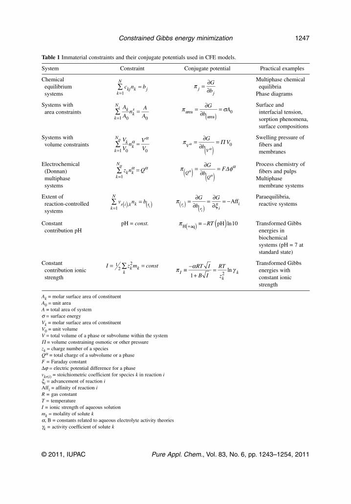
Table 1 Immaterial constraints and their conjugate potentials used in CFE models.

System Constraint Conjugate potential Practical examples

Chemical Multiphase chemicalequilibrium equilibriasystems Phase diagrams

Systems with Surface andarea constraints interfacial tension,

sorption phenomena,surface compositions

Systems with Swelling pressure ofvolume constraints fibers and

membranes

Electrochemical Process chemistry of(Donnan) fibers and pulpsmultiphase Multiphasesystems membrane systems

Extent of Paraequilibria,reaction-controlled reactive systemssystems

Constant pH = const. Transformed Gibbscontribution pH energies in

biochemicalsystems (pH = 7 atstandard state)

Constant Transformed Gibbscontribution ionic energies withstrength constant ionic

strength

Ak = molar surface area of constituentA0 = unit areaA = total area of system σ = surface energy Vk = molar surface area of constituentV0 = unit volumeV = total volume of a phase or subvolume within the system Π = volume constraining osmotic or other pressure zk = charge number of a speciesQα = total charge of a subvolume or a phase F = Faraday constantΔϕ = electric potential difference for a phasevkr(i) = stoichiometric coefficient for species k in reaction iξi = advancement of reaction iAffi = affinity of reaction iR = gas constantT = temperatureI = ionic strength of aqueous solutionmk = molality of solute kα, B = constants related to aqueous electrolyte activity theoriesγk = activity coefficient of solute k



c n bkjk

N

k j=∑ =

1

π jj

G

b= ∂

∂

A

An

A

Ak

k

N

kss

01 0=∑ = π σarea

area

= ∂∂

=( )G

bA0

V

Vn

V

Vk

k

N

k01 0=

∑ =α α

απ α

αV

V

G

bV= ∂

∂=

( )Π 0

z n Qkk

N

k=∑ =

1

α α α π φαα

αQ

Q

G

bF( ) ( )

= ∂∂

= Δ

v n br i k kk

N

i( ) ( )=

=∑ , r1

πξr

r ii

ii

G

b

G( ) ( )

= ∂∂

= ∂∂

= −Aff

πH aq pH+( ) ≡ ( )– lnRT 10

I z m constkk

k= =∑12

2

π α γIk

kRT I

B I

RT

z≡ −

+=

1 2ln

CALCULATION EXAMPLES

Surface and interface energies of mixtures

Computation of the surface energy of liquid mixtures provides a simple introductory example of the useof immaterial constraints in the Gibbsian multicomponent systems. Existence of a surface monolayer,being in equilibrium with the bulk system (the surface curvature effects are neglected), is assumed. It iscustomary to separate the contributions of the bulk (b) and surface (s) contributions to the Gibbs energyas follows [23]:

(9)

where Ak is the molar surface area of species k and σ the surface tension in the system. Both the bulkand surface parts have the same constituents with the same index number k referring to same species ineq. 9. The respective conservation equations corresponding to the condition (eq. 2) for the equilibriumsurface system are

(10)

(11)

Equation 10 is the mass balance equation for the components, presented in terms of the stoichio-metric numbers (ckj), which appear as elements in the respective conservation matrix C (see, e.g.,[1,3,20]). As the surface area of the equilibrium system is also a conserved quantity, eq. 11 is then

derived from the condition , where A is the total surface area. To reach an analogous

(dimensionless) form with the mass balance constraint (eq. 10), the unit area [m2/mol] normalizationconstant A0 has been used. The condition (eq. 11) is only applicable for the surface phase, and thus thesummation over phases is irrelevant and merely shown to indicate the formal similarity of the two con-ditions.

When comparing eqs. 7 and 9 combined with eq. 11 one obtains for the surface energy of the mix-ture

σ A0 = πj=NC'+1 (12)

The subscript j = NC' +1 indicates the additional immaterial “surface” component of the system.This result can also be derived from eq. 5 by using eqs. 9–11 in the minimization procedure as wasshown in [25,26]. The additional elements of the conservation matrix are the Ak/A0 ratios as deduced ineq. 11. The molar surface areas of the pure substances can be derived from the respective molar vol-umes [27] or by using estimates of the molecular diameters ([24] p. 212). The constant A0 can be cho-sen arbitrarily, but for practical calculation reasons it is advantageous if the ratio Ak/A0 has a numericalvalue close to unity, being of the same order of magnitude as the stoichiometric coefficients appearingin the conservation matrix.

To perform the surface tension calculations with a Gibbs energy minimizing program, the inputdata must be arranged in terms of the standard state and excess Gibbs energy data of chemical poten-tials of the surface system. The relation between the appropriate standard states was originally deducedby Butler [28]

μk°,s = μk° + Ak σk (13)



1248

G n n A nkb

k

N

kb

ks

k

N

ks

kk

N

ksb s s

= + += = =∑ ∑ ∑μ μ

1 1 1

c n b j lkjk

N

k jα α

α

α

==∑∑ − = = …

110

Ω( )1,2

A A n A Akk

N

kα α α

α

α

01

01

0( ) − ===∑∑

Ω

A n Akk

N

k=∑ =

1

s s

The necessary input for a Gibbsian surface energy calculation thus must include not only the stan-dard state and thermodynamic activity (excess Gibbs energy) data for the constituents of the bulk andsurface phases but also the data for surface tensions of the pure substances (σk) as well as their molarsurface areas (Ak). As a simple calculation example, the melt of silver (Ag) and lead (Pb) is presentedin Fig. 1. The figure shows the calculated surface tension and the composition of the surface phase interms of the mole fraction of lead in the bulk. The excess Gibbs energy is formulated as aRedlich–Kister polynomial with parameters assessed for the Ag–Pb bulk binary system [25].

The CFE method applies to surface and interfacial energy problems in a wide range of tempera-tures and mixtures ranging from binary and ternary melts to aqueous-organic and organic systems andhave been further discussed, for example, in [26,32,33].

Electrochemical Donnan-potential in multiphase systems

When two aqueous solutions at the same temperature are separated with a semi-permeable interface,which allows transport of some ions but not others, the Donnan equilibrium is formed in the system ofthe two compartments ([24] p. 307). The system consists of two aqueous phases with water as solventand mobile and immobile ions as solute species. Gas as well as precipitating solids affecting the solu-tion equilibria may yet be present. The aqueous solutions in both compartments remain electrically neu-tral. The essential feature of the Donnan equilibrium is that due to the macroscopic charge balance inthe separate compartments, immobility of some of the ions will cause an uneven distribution also forthe mobile ions. This distribution strongly depends on the acidity (pH) of the system in such caseswhere dissociating molecules in one of the compartments (being immobile acidic groups typically pres-ent, e.g., in the fibrils of cellulose fibers) may release mobile hydrogen ions, while their respective(large or bound) counter anions remain immobile due to the separating membrane interface or chemi-cal bonding.



Fig. 1 Calculation of the surface tension of a non-ideal binary system. The excess Gibbs energy (GE) is includedas the Redlich–Kister polynomial and the GE(surface) = 0.83GE(bulk) as deduced from the reduced coordinationnumber between atoms in the surface region [31]. Experimental values are from [29,30].

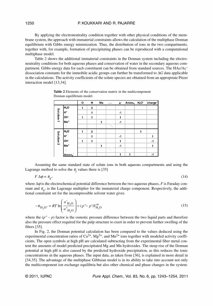
By applying the electroneutrality condition together with other physical conditions of the mem-brane system, the approach with immaterial constraints allows the calculation of the multiphase Donnanequilibrium with Gibbs energy minimization. Thus, the distribution of ions in the two compartments,together with, for example, formation of precipitating phases can be reproduced with a computationalmultiphase model.

Table 2 shows the additional immaterial constraints in the Donnan system including the electro -neutrality conditions for both aqueous phases and conservation of water in the secondary aqueous com-partment. Gibbs energy data for each constituent can be obtained from standard sources. The HAc/Ac–

dissociation constants for the immobile acidic groups can further be transformed to ΔG data applicablein the calculations. The activity coefficients of the solute species are obtained from an appropriate Pitzerinteraction model [13,34].

Table 2 Elements of the conservation matrix in the multicomponentDonnan equilibrium model.

Assuming the same standard state of solute ions in both aqueous compartments and using theLagrange method to solve the πj values there is [35]

F Δϕ = πq" (14)

where Δϕ is the electrochemical potential difference between the two aqueous phases, F is Faraday con-stant and πq" is the Lagrange multiplier for the immaterial charge component. Respectively, the addi-tional constraint set for the incompressible solvent water gives

(15)

where the (p'' – p) factor is the osmotic pressure difference between the two liquid parts and thereforealso the pressure effect required for the pulp structure to exert in order to prevent further swelling of thefibers [35].

In Fig. 2, the Donnan potential calculation has been compared to the values deduced using theexperimental concentration ratios of Ca2+, Mg2+, and Mn2+ ions together with modeled activity coeffi-cients. The open symbols at high pH are calculated subtracting from the experimental fiber metal con-tent the amounts of model predicted precipitated Mg and Mn hydroxides. The steep rise of the Donnanpotential at high pH is also caused by the predicted hydroxide precipitation, as this reduces the ionicconcentrations in the aqueous phases. The input data, as taken from [36], is explained in more detail in[34,35]. The advantage of the multiphase Gibbsian model is in its ability to take into account not onlythe multicomponent ion exchange equilibria but also other chemical and phase changes in the system.



1250

− =⎛

⎝⎜⎜

⎞

⎠⎟⎟

= −πH OH O

H OH O22

2

2

'' ln'

"( '' ')RT

a

ap p V m

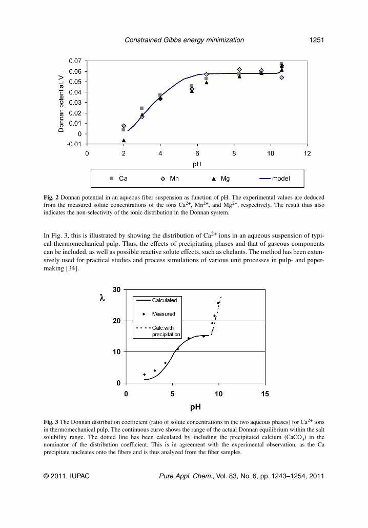
In Fig. 3, this is illustrated by showing the distribution of Ca2+ ions in an aqueous suspension of typi-cal thermomechanical pulp. Thus, the effects of precipitating phases and that of gaseous componentscan be included, as well as possible reactive solute effects, such as chelants. The method has been exten-sively used for practical studies and process simulations of various unit processes in pulp- and paper-making [34].



Fig. 2 Donnan potential in an aqueous fiber suspension as function of pH. The experimental values are deducedfrom the measured solute concentrations of the ions Ca2+, Mn2+, and Mg2+, respectively. The result thus alsoindicates the non-selectivity of the ionic distribution in the Donnan system.

Fig. 3 The Donnan distribution coefficient (ratio of solute concentrations in the two aqueous phases) for Ca2+ ionsin thermomechanical pulp. The continuous curve shows the range of the actual Donnan equilibrium within the saltsolubility range. The dotted line has been calculated by including the precipitated calcium (CaCO3) in thenominator of the distribution coefficient. This is in agreement with the experimental observation, as the Caprecipitate nucleates onto the fibers and is thus analyzed from the fiber samples.

Systems constrained by the extent of reaction

As shown with the above examples, the CFE minimization generally results in another undeterminedLagrange multiplier, which gives the desired property as a constraint potential. The same technique canbe used for a fixed amount of a virtual system component, which then serves to limit the time-depend-ent extent of a selected chemical reaction or phase change. The additional Lagrange multipliers thenappear as the non-zero affinities of the kinetically constrained non-equilibrium reactions [20,37]. Thisfeature enables the use of the Gibbsian multiphase method effectively, e.g., in the simulation of variouschemical and combustion processes [38–40]. Such applications often include mass and heat transfermodels and other process-specific features which are beyond the scope of this text. From the thermo-dynamic point of view, an appropriate example is, however, the construction of reactive phase diagramsfor systems where the chemical change appears at a given (non-equilibrium) extent of reaction, whilethe respective phase composition is at equilibrium.

Chemical reaction kinetics can often prevent equilibriation in chemically reactive fluid mixtures,particularly at low temperatures and in conditions where the phase separation is to take place in a shortresidence time [41]. The well-known ethanol-acetic acid, water-ethylacetate system serves as a viableexample [42] and was chosen to illustrate the respective calculation by using the constrained Gibbsenergy technique.

As physical components of the model system, those corresponding to ethanol, acetic acid, andwater were selected. Yet, the same result can be obtained with the elements (C, H, and O) as physicalcomponents. Additional immaterial constraint was applied to the ethyl acetate species allowing the con-trol of the advancement of the esterification reaction. The standard-state chemical potentials from [43]were adjusted by using the vapor pressure data from several sources [44–47]. The vapor phase wasregarded as an ideal gas including the acetic acid dimer, while the liquid mixture is modeled using theUNIFAC data [48].

Dew and bubble temperatures plotted in terms of the feed composition and reaction advancementas two-dimensional surfaces are shown in Fig. 4 (left). For depicting vapor–liquid equilibria, it is morerelevant to compare the vapor and liquid phase not with the same reaction advancement of the esterifi-cation reaction, but the two phases with equal affinity for the reaction [41]. It is straightforward to per-form the respective isoaffinity calculation, as in the CFE method the Lagrange multiplier adjacent to theextent of a kinetically constrained reaction provides directly the non-equilibrium affinity [37,49]. Theresult is shown in Fig. 4 (right) where one of the coordinates is the advancement of the reaction in theliquid phase.



1252

Fig. 4 Dew and bubble point surfaces for the reactive ethanol acetic acid system. The chemical reaction is theesterification of acetic acid with ethanol: CH3CH2OH + CH3COOH → CH3CH2COOCH3 + H2O. The graphs areproduced by using one of the axis either as reaction advancement (left) or as reaction advancement in the liquidphase together with isoaffinity condition (right).

CONCLUSION

The use of immaterial and virtual constraints provides a thermodynamically consistent extension of theGibbs energy minimization calculation for multiphase systems. Adjusting the thermodynamic systemfor constrained Gibbs energy calculations appears mathematically identical to the procedure involvedin the conventional Gibbsian equilibrium calculations. The immaterial constraints must be defined inadvance for the calculation system and be included as parts of the conservation matrix. The immaterialconstraints and their conjugate potentials are principally those which may appear in the generalizedGibbs energy function or, alternatively, may be derived from it by using the appropriate Legendre trans-form. Within a few years, the new method has found applications in solving surface and interfacial ener-gies of mixtures, electrochemical potentials of membrane systems, and non-equilibrium affinities forreactive systems. The consistent thermodynamic basis of the method suggests that new interesting top-ics may appear in various fields of process chemistry and materials science as well as in, for example,biochemical pathway analysis.

REFERENCES

1. W. R. Smith, R. W. Missen. Chemical Reaction Equilibrium Analysis: Theory and Algorithms,Krieger, Malabar, FL (1991).

2. S. Gordon, B. J. McBride. Computer Program for Calculation of Complex EquilibriumCompositions and Applications, NASA Reference Publication 1311 (1994).

3. G. Eriksson. Acta Chem. Scand. 25, 2651 (1971).4. M. Hillert. Bull. Alloy Phase Diagrams 2, 265 (1981). 5. L. Kaufman, H. Bernstein. Computer Calculation of Phase Diagrams, Academic Press, New

York (1970).6. K. Hack (Ed.). The SGTE Casebook: Thermodynamics at Work, 2nd ed., p. 14, Woodhead,

Cambridge (2008).7. S. M. Walas. Phase Equilibria in Chemical Engineering, Butterworth, Stoneham, MA (1985). 8. A. L. Ballard, E. D. Sloan. Fluid Phase Equilib. 218, 15 (2004).9. D. V. Nichita, S. Gomez, E. Luna. Comput. Chem. Eng. 26, 1703 (2002).

10. E. Königsberger, G. Eriksson. J. Solution Chem. 28, 721 (1998). 11. E. Königsberger. Pure Appl. Chem. 74, 1831 (2002).12. J. Lindgren, L. Wiklund, L.-O. Öhman. Nordic Pulp Paper Res. J. 16, 24 (2001).13. P. Koukkari, R. Pajarre, H. Pakarinen. J. Solution Chem. 31, 627 (2002).14. P. Sundman, P. Persson, L.-O. Öhman. J. Colloid Interface Sci. 328, 248 (2008).15. M. Lampinen, J. Vuorisalo. J. Electrochem. Soc. 139, 484 (1992).16. R. A. Alberty. J. Phys. Chem. 93, 3299 (1989).17. J. C. Keck, D. Gillespie. Combust. Flame 17, 237 (1971).18. J. C. Keck. Prog. Energy Combust. Sci. 16, 125 (1990).19. P. Koukkari. Comput. Chem. Eng. 17, 1157 (1993).20. P. Koukkari, R. Pajarre. CALPHAD 30, 18 (2006).21. R. Pajarre, P. Blomberg, P. Koukkari. Comput.-Aided Chem. Eng. 25, 883 (2008).22. P. B. A. Blomberg, P. Koukkari. Math. Biosci. 220, 81 (2009).23. R. Alberty. Pure Appl. Chem. 73, 1349 (2001).24. E. A. Guggenheim. Thermodynamics, p. 335, North-Holland, Amsterdam (1977).25. P. Koukkari, R. Pajarre, K. Hack. Int. J. Mater. Res. 98, 926 (2007).26. R. Pajarre, P. Koukkari, T. Tanaka, Y. Lee. CALPHAD 30, 196 (2006). 27. E. T. Turkdogan. Physical Chemistry of High-Temperature Technology, p. 96, Academic Press,

London (1980).28. J. A. V. Butler. Proc. R. Soc., London, A 135, 348 (1932).



29. J. C. Joud, N. Eustathopoulos, P. Desse. J. Chim. Phys. 70, 1290 (1973). 30. G. Metzger. Z. Phys. Chem. 211, 1 (1959). 31. T. Tanaka, K. Hack, T. Ida, S. Hara. Z. Metallkunde 87, 380 (1996).32. R. Pajarre, P. Koukkari. J. Colloid Interface Sci. 337, 39 (2009).33. R. Pajarre, P. Koukkari, T. Tanaka. To be published.34. P. Koukkari, R. Pajarre, E. Räsänen. In Chemical Thermodynamics for Industry, T. M. Letcher

(Ed.), pp. 23–32, Royal Society of Chemistry, Cambridge, UK (2004).35. R. Pajarre, P. Koukkari, E. Räsänen. J. Mol. Liq. 125, 58 (2006).36. M. Towers, A. M. Scallan. J. Pulp Paper Sci. 22, J332 (1996).37. P. Koukkari, R. Pajarre, P. Blomberg. Pure Appl. Chem. 83, 1063 (2011).38. P. Koukkari, I. Laukkanen, S. Liukkonen. Fluid Phase Equilib. 136, 345 (1997).39. M. Janbozorgi, S. Ugarte, H. Metghalchi, J. C. Keck. Combust. Flame 156, 1871 (2009).40. R. Gani, T. S. Jepsen, E. S. Pérez-Cisneros Comput. Chem. Eng. 22, Suppl., S363 (1998).41. G. Maurer. Fluid Phase Equilib. 116, 39 (1996). 42. A. Toikka, M. Toikka, Yu. Pisarenko, L. Serafimov. Theor. Found. Chem. Eng. 43, 129 (2009).43. A. Roine, Outokumpu. HSC Chemistry® for Windows, Version 4.1 (1999).44. A. C. Vawdrey, J. L. Oscarson, R. L. Rowley, W. V. Wilding. Fluid Phase Equilib. 222–223, 239

(2004).45. D. Ambrose, J. H. Ellender, C. H. S. Sprake, R. Townsend. J. Chem. Thermodyn. 9, 735 (1977).46. P. Sauermann, K. Holzapfel, J. Oprzynski, F. Kohler, W. Poot, T. W. de Loos. Fluid Phase Equilib.

112, 249 (1995).47. H. S. Wu, S. I. Sandler. J. Chem. Eng. Data 33, 157 (1988).48. B. E. Poling, J. M. Prausnitz, J. M. O’Connell. Properties of Gases and Liquids, 5th ed., McGraw-

Hill (2001).49. P. Koukkari, R. Pajarre. Comput. Chem. Eng. 30, 1189 (2006).



1254

a gibbs energy minimization method for constrained and...

Documents