Purdue University Purdue University

Purdue e-Pubs Purdue e-Pubs

Department of Computer Science Technical Reports Department of Computer Science

1993

A Geometric Constraint Solver A Geometric Constraint Solver

William Bouma

Ioannis Fudos

Christoph M. Hoffmann Purdue University, cmh@cs.purdue.edu

Jiazhen Cai

Robert Paige

Report Number: 93-054

Bouma, William; Fudos, Ioannis; Hoffmann, Christoph M.; Cai, Jiazhen; and Paige, Robert, "A Geometric Constraint Solver" (1993). Department of Computer Science Technical Reports. Paper 1068. https://docs.lib.purdue.edu/cstech/1068

This document has been made available through Purdue e-Pubs, a service of the Purdue University Libraries. Please contact epubs@purdue.edu for additional information.

brought to you by COREView metadata, citation and similar papers at core.ac.uk

provided by Purdue E-Pubs

A GEOMETRIC CONSTRAINT SOLVER

William BoumaIoannnis Fudos

Christoph HoffmannJillzhen CaiRobert Paige

eSD·TR·93·054August 1993

A Geometric Constraint Solver

William Bouma- Ioannis Fuclos t Christollh Hoffmann·Department of Computer Science, Purdue University

West Lafayette, IN 47907-1398

Jiazllen Cai1 Robert Paige}Department of Computer Science, Courant Institute

251 Mercer Str., New York, NY 10012

Report CSD_'rlt_n.05t, Aug.. ' 19931

Abstract

We report on the development of a two-dimensional geometric COll­

straint solver. The solver is a major component of a lIew generation ofCAD systems that we are developing based on a high-level geometry rep­resentation. The solver uses a graph-reduction directed algebraic approach,and achieves interactive speed. We describe the architecture of the solverand its basic capabilities. Theil) we discuss ill detail holV to extend thescope of the solver, with special emphasis placed all the theoretical alldhuman fadors involved in finding a solution - in an eXJlonenlially largesearch space - so that the solution is appropriate to the application andthe way offincling it is intuitive to an untrained user.

·Supported in part by ONR contract N00014-90-J-1599, by NSF' Granl COA 92-2.'3.502, andby NSF Grant ECD 88-03017.

lSupported by a David Ross fellowship.ISupportcd in part by DNR contract NOOOl4-90-J-1890, by AFDSR ~ralLt 91-0308, and by

NSF grant MIP 93-00210.§This report and others are available via anonymous ftp to artlulT.cs.purdue.edu, i.ll direc­

tory pub/emit and subsidiaries

1 Introduction

Solving a system of geometric constraints is a problem that has been consid­ered by several communities, and using different approaches. For example, thesymbolic computation community has considered the ~etleral problem, in thecontext of automatically deriving and proving theorems from analytic geometry,and applying these techniques to vision problems [9, 14,26,27]. The geometriemodeling community has considered the problem for the purpose of developingsketching systems ill which a rough sketch, annotated with dimension and con­straints, is instantiated to satisfy all constraints. This work will be reviewed inthe next section. The applications of this approach aTe in mechanical engineer­ing, and, especially, in manufacturing.

With this work, we have mainly manufacturing applications in mind. Ourpurposes aud goals are as foUows:

1. We develop a constraint solver in which the information flow between theuser interface and the underlying solver h<l.'> been formalized by a high-levelrepresentation that is neither committed to the particular capabilities ortechnical characteristics of the solver, nor is dependent on the interface.Such a representation becomes the basis for archiving sketches in a neutralformat, with the ability to retrieve the archived sketch and edit it ­possibly in a different system with a different solver [24, 23]. Our solutionis also a building block for a larger project of developing a new geuerationof CAD systems based on a neutral, high-level geometry representationthat expresses design intent aud preserves the ability to redesign.

2. We explore the utility of several different general-purpose and interoperat­lng rapid prototyping languages and systems for developing specific toolsfor experimenting conveniently with a variety of ideas and approaches toconstraint solving. Aside from well-known special purpose tools such asLEX and Yacc [25J, our constraint solver also make'S use of the high levellauguage SETL2 [45] to specify complex combinatorial algorithms andthe transformational system A PTS [12] to perform syntactic analysis andsymbolic manipulation of geometrical constraint spedfications.

3. We study a number of neglected aspects of constraint solving, in par­ticular the process of redirecting the solver to a different solution of awell-constrained sketch, and to devise generic techniques for extendingthe capabilities of the solver willie preserving interactive speed.

This paper reports substantial progress in all three problem dimensions, andidentifies a number of open issues that remain.

2

2 Approaches to Geometric Constraint Solving

We consider only well-constraiIled, two-dimensional sketchl's formed [rom points,lines, circles, segments and arcs. Constraints are explicit dimensions of distancesand angles, as well as constraints of paraUelisIll, incidence, perpendicularity, tan­gency, concentricity, collinearily, and prescribed radii. We exclude relations ondimension variables and inequality constraints. In partir.uli:tr, the uscr spedfLesa rough sketch and adds to it geometric and dimensional constraints that arenormally not yet satisfied by the sketch. The sketch only has to be topologi­cally correct. The constraint solver determines from the sketch the geometricelements that aTe to be found, and processes the constraints to determine eachgeometric element such that the constraints are satisfied.

Our constraint solver is variational. That is, the solver is not obliged toprocess the constraints in a predetermined sequence, and thc constraints speci­fied by the user are not !)arametric in the sense that they IllIISt be determine(1serially, each as an explicit function of the llreviolls constraints. This is anal­ogous to writing the constraints in a declarative language, where tllc solutionis independent of the order in which the constraints are written down. Thisgreatly increases the generality of the constraint solving llroblem, and demandssolvers that are based on advanced mathematical concepts.

While the users of geometric constraint solving systems t1tink geometricallyand express themselves with visual gestures, the underlyin~ constraint solverstYllically work with a different internal rellresentation. Most users will be quiteunaware of the nature of the underlying representation, and of the internalworkings of the constraint solver. Coupled with the fact that a well-constrainedgeometric constraint problem has, in general, exponentially many solutions,only one of which satisfies tIle llser's intent, cOllStl'aint solvers therefore have toaddress two distinct tasks:

1. Deterntine whether the problem can be solved and if so, how.

2. Among the possible solutions, identify the one the user has intended.

Most of the literature assumes tacitly that the second task is easy to discharge.In Section 5, we question tltis assumption and show WIlY Task 2 is difficult forapplications.

Before describing our approae1l to Task 1, it is useful to characterize otherapproaches in the literature.

2.1 Numerical Constraint Solvers

In general numerical constraint solvers, the constraints are translated into asystem of algebraic equations and are solved using an iterative method. When

3

base(] on Newton iteration, such solvers require good initial values, which impliesthat the initial sketch must almost satisfy all constraints already. The solversare quite general, and are capable of dealing with overconstrained, consistentconstraint problems. Many constraint solvers switch to iterative methods insituations where the given configuration is not solvable by the native method.

Nonlinear systems have an exponential number of solutions, but Newtoniteration will find only one. Numerical solvers based on Newton iteration aretherefore inappropriate when the initial sketch is only topologically correct, orwhen the solver locks into a solution that is unsuited to the application and hasno method with which to find more suitable alternatives.

Sketchpad [51] was the first system to use the method of numerical relax­ation. Relaxation is slow but quite general. Many systems like ThingLab [3]and Magritte [22] can do relaxation as an alternative to some other method. In(2] a projection method is presented for finding a new solution that minimizesthe Euclidean distance between the old and the new solution.

Newton-Raphson iteration has been used in a number of systems, and isfaster than relaxation, but it may converge to the wrong solution. Unfortu­nately, when this happens, the user has no recourse to instruct the solver tofind alternatives. Juno [37] uses the original sketch as initial state. The CPSMsystem of Solano and Brunet [47] also uses a numerical solver that first deals withsequential constraints and then solves circularly interdependent constraints.

A modification of Newton-Raphson was developed in [;l5], where an improvedway for finding the inverse .Jacobi matrix is presented. Furthermore, the paperproposes dividing the constraint matrix into submatrices, witll the potential ofproviding the user with information about the constraint structure of the sketch.Although this information is usually quantitative and not very specific, it mayhelp the user make modifications if the solver fails. A method that representsconstraints by an energy function and then searches for a local minimum usingthe energy gradient is presented in [56].

2.2 Constructive Constraint Solvers

This clMs of constraint solvers is based on the fact that most configurationsin an engineering drawing are solvable by ruler, compass and protractor, orusing another, less classical repertoire of construction steps. In these metbods,the constraints are satisfied constructively, by placing geometric elements insome order. This is more natural for the user and makes the approaclJ suitablefor interactively debugging a sketch that cannot be solved or has been solvedunsatisfactorily, froIll an application point of view.

4

2.2.1 Rule-Constructive Solvers

One version of the constructive approach uses rewrite rules to dlscover andexecute the construction steps. We call this approach rule-Coll8truclive solving.Although a Logic Programming style of programming is a ~ood apllroach forprototyping and experimentation, the extensive computations searching andmatching rewrite rules constitute a liability.

Bruderlin and Sohrt [6, 46J solve constraints in thls way and inc.orporatethe Knuth-Bendix critical-pairs algorithm [29]. They show that their methodis correct and solves all problems that can be constrncted usinp; ruler and com­pass. The method can also be proved to confmll geometric theorems that areprovable in their system of axioms. Bruderlin and Sohl't have implemented auexperimental constraint solving system in Prolo/!;. They do not address how todevise rules for determining automatically which of tIle possible solutions is theone the user intended.

Aldefeld [1] uses a forward chaining inference mechanism. He assumes thatlines are directed, and formulates ad(litional rules that rE'strict the number ofpossible solutions. A similar method is presented in [52], where handlin/!; of over­constrained and underconstrained cases is given special consideration. Sunde in[50] also uses a rule-constructive method but has different rulE'S for represent­ing d.irected distance and lmdirected distance, thus adding f1pxlbility for dealingwith the root identification problem discussed in Section .5. In [58] the problemof nonuniqlle solutions is handled by imposing all order on triples of geometricelements. A detailed descrl]ltion of a complete set of rules for 20 design canbe found in [.5fi], where the scope of the rules is also characterized. Finally, atechnique called Meta-level Inference is introduced in [10]. The paper claimsthat this technique, combined with multiple sets of rulE'S and their seleetive ap­plication, reduces the searcll space. The method has lJeen applied in PRESS[10], a Jlrogram for algebraic manipulation.

2.2.2 Graph-Constructive Solvers

Another version of the constructive a]lproach has two phases. Durinp; the firstphase, the graph of constraints is analyzed and a sequence of c.onstruction stepsis derived. During the second phase, the construction steps arC! carrled out toderive the solution. We call this approach gmph-con,~t"lctivcsolving. It is fast,more me~hodical than the rule-constructive approach, and is llroved to be sound.However, as the repertoire of possible constraints increases, t.he graph-analysisalgorithm has to be modified.

Fitzgerald [20] follows the approach of dimensioned trees by Requicha [43].Only horizontal and vertical distances are allowed in this method and so theapplicability of the method is lim.ited. Todd in [53) generalized the dimension

5

trees of Requicha. Owen in [38] presents an extension of this principle to includecircularly dimensioned sketches, and DCM [19J is a commercial constraint solverusing this method.

Since our basic algorithm is based on many of the ideas of [38], we describe *** ChangesOwen's solvers in more detail. The constraint solver described in [38J is a graph-constructive solver in which the constraint graph is analyzed for triconnectedcomponents. Each trkonnected component is reduced to a number of elementsthat interact with other components, and a determination is made how the var-ious geometric elements whose nodes are in ead graph component fit together.Thereafter, each component can be separately determined. This procedure. isrecursive in that once components have been reduced, they in turn can becomemembers of triconnected components in the reduced graph. A key aspect of thesolver is that only constraint configurations are considered that can be solvedusing ruler-and-compass construction steps. Algebraically, this is equivalent tosolving only quadratic equations, so that the specific coordinate computationsdo not require sophisticated mathematical computations. In [3R] a proof is giventhat the solver is complete for ruler-and-compass constructible point configura-tions with prescribed distances that are algebraically independent.

DCM [19] shares with the algoritllln of [38] the characteristic that it begins *** Changesby determ.ining the interaction of geometric element groupings before filling inthe individual elements in each group. In addition, we infer that the commercialversion has a significant number of additional flues and transformations thatcan be applied to the constraint graph in order to extend the scope of the basicalgorithm. In many cases, the gra])h reduction requires linear time only.

Kramer [32] uses a similar approach. However, instead of determining theequations of the geometric elements at each construction step, Kramer deter­mines coordinate transformations that successively place points and associatedcoordinate frames relative to each other subject to constraints. Kramer's COll­straint solver is for 3D and deals with constraints that arise in kinematics andcharacterize basic joint types. Thus, a revolute constraint matches the pointsalHI aligns a pair of coordinate axes, allowing a sillgle degree of freedom, a rota­tion about the aligned axes. Complex geometric elements are placed implicitlyby choosing a suitable number of points on them whose cOOl"dinate frames arerelatively fixed, and then placing each point.

2.3 Propagation Methods

Constraint propagation was a popular approach in early constraint solving sys­tems. The COllstraints are first translated into a system of equations involvingvariables and constants, and an undirected graph is created whose nodes arethe equations, variables and constants, and whose ed~es represent whether avariable or constant OCCllrs in an equation. The method then attempts to direet

6

the graph edges so that every eqnation can be solved in turn, initially only fromthe constants. To succeed, various propagation techll.iql1es have been tried, Imtnone of them is guaranteed to derive a solution when one exists. For a review,eo [33, 461.

Sketchpad [51] uses propagation of degrees of freedom and propagation ofknown values. Pro/ENGINEER [5, 40J uses propagation of known values. Prop­agation of known values is the inverse process of the propagation of degrees offreedom. Propagation of degrees of freedom is a more abstract method thatessentially does a graph reduction. In the propagation of known values, we canaccount for special values and therefore make the method slightly more pow­erful than pure propagation of degrees of freedom. Both methods are global,unstable, and do not work for cyclically dimensioned sketches_

CONSTRAINTS [48] uses retraction, wl1ic1l is a localized version of propa­gation of known values that stores information about each variable's interdepen­dencies. A similar technique is used in [34]: First, known values arc propagatedlocally. Then, the remaining simultaneous constraints are solved if they forma linear system of equations. In general, retraction is faster but less powerfulthan propagation of known values.

Graph transformation is sometimes used in conjunction with some prop­agation method. In pure graph transformation, some subgraphs of the con­straint graph are identified and are replaced by simVler subgraphs. Bertrand,described in [33], is a general-purpose constraint specification language, andis hnplemented using a propagation method in conjunction with an inferencemechanism. LeIer calls this technique augmented tC1"11l l'cwl-iting. In essence,augmented term rewriting is a graph transformation mechanism Ilsing termrewriting rules. Additionally, assignments are supported, as is variable typing,and these additions make augmented term rewriting more expressive tha11 theterm rewriting mechanism of pure PROLOG.

Th·lIlgLab uses the Blue and Delta Blue algorithms described in [3,21], thatare based on a local propagation of degrees of freedom within the consLraintgraph. Magritte [22] employs propagation to transform the undirected con­straint graph, and then uses breadth-first search to derive all solutions.

2.4 Symbolic Constraint Solvers

The constraints are transformed into a system of algebraic equations. Thesystem is solved wiLh symbolic algebraic methods, such as Grabner's bases, e.g.,[9], or the Wu-llitt method (57, 14]. Both methods can solve general nonlinearsystems of algebraic equations. The methods have also been llsed in mechanicalgeometry theorem proving [16,17, 15,26].

In [30, 31J, Kondo considers the addition and deletion of constraints byusing the Buchberger's Algorithm [7, 8] to derive a polynomial that gives the

7

GraphicalUser Interface

k.,=;;:>IErep I-.,----;"'~I Constraint Solver

Figme 1: Architecture of the Constraint Solver

relationship between the deleted and added constraints.

2.5 Hybrid Solvers

Often, constraint solving systems use a combination of the abovp. methods. Onemethod 1s attempted, and if it does not succeed, another one is tried. Themain (lifficulty is that some of the methods Illay require f'xponential time beforegiving a negative response.

3 The Constraint Solving System

3.1 Information Flow and Rationale

The overall architecture of the constraint solver is as shown in Figure 1. Theuser draws a sketch and annotates it with geometric constraints. The allowedconstraints include relations such as tangency, perpendicularity, etc, and explicitdimensioning of angles and distances. Excluded for noW are relations betweendimension variables. Additional capabilities include interacting with the solverto identify a different, valid solution. The geometric elements available at thistime are segments, points, and circular arcs. Auxiliary lines, points and circlesmay also be defined.

The user interface translates the specificatiOll illto a textual langua~e thatis a faithful recor<1 of the problem. Although the user could cdit tIlls textualproblem specification, this is unnecessary, because the specification is editedand updated automatically from the visual gestures by the user interface. Thelanguage has been designed to adlleve the objectives of [24]- a neutral problemspecification that makes no assumptions about tbe architecture ofthe underlyingconstraint solving algoritbm. Thus, it is quite easy to federate Owen's solver [38],or any other constraint solver capable of handling the geometric configurationswe consider.

The textual problem specification is handed to the constraint solver enginewhich translates the constraints into a graph, and, as described later, solvesthem by graph reductions that govern the workings of all al,e;ebraic, variational

8

constraint solver. The solver capabilities are the consequellCf' of speciIic con­struction steps that have been implemented. If a particular constraint problemcan be solved using the known construction steps, then Ollr solver will find a so­lution. Where the construction steps involve ruler-and-compass constructions,only quadratic equations need to be solved_ But some wllstruction steps arepermitted that are not ruler-and-compass, and in those situations the roots ofa univariate polynomial are found numerically. In those situations, the polyno­mial ha.<> been precomputed except for the coefficients which are functions of thespecific constraint values_ The solver architecture is optimized for speed subjectto the strict requirement that the information flow between user interface andsolver does not depend on the internals of either component.

In the worst case, a well-constraillcd geometric problem has exponentiallymany solutions in the number of constraints. This is because the solutionscorrespond to the algebraic set of a zero-dimensional ideal whose generatingpolynomials arc nonlinear. Our solver can determine all possible solutions. Butdoing so every time would waste time and overwhelm the user. So, certainheuristics, described later, narrow down the solutions to a TIna] configurationthat corresponds to the intended solution with high probability. It would 1)enice if methods could be devised that identify the solution tIle user intendedevery time. But even in very simple situations, additional information thatwould help doing so would lead to provably intractable problems. This wouldbe incompatible with our goal of interactive speed. Instead, we have developeda paradigm for finding the right solution by using the solver interactively whenits automatic heuristics are insufficient.

Our system will be a component of a constraint-driven varialional CAD sys­tem based on a high-level, declarative, ed.itable geometry representation (Erep)as discussed in [24, 23]. Such an overall archileclure poses several challenges.One of them is efficient variational constraint solving, and we address this prob­lem here. Another, key challenge is to formulate the langu<Lge in a neutral way,committing it neither to the particulars of the user interface nor orthe solver al­gorithms. This is a more subtle challenge because the way in which dimensionsare displayed in the sketch has to make some assumptions about the capabilitiesof the IIser interface. Likewise, interacting with the solver to find alternativesolutions requires conceptualizing the solution process 1n a way that makes noassumptions about how they are found. Here, we assume only that the solveris capable of undoing the last placement operation, and can look for a differ­ent placement of a geometric element. The textual protoeol for communicatingthese matters is encapsulated.

9

3.2 System Implementation

The two-dimensional geometrical design system has two main components, agraphical interface and a constraint solver engine. The graphical interface is aC++ program [49] that lnteracts with X Windows in order to allow the userto sketch a drawing using labeled points, lines, circles, etc. The user is alsoexpected to supply initial constraints lletween these ~('onJ(>.tric elements. Thisinitial design is turned into an Erep specification and is passed as text to theconstraint solver.

The solver 1s wriUen using two novel software tools - tIle APTS transfor­mational programmillg system [12] and the high-level langltage SETL2 [45] ­each having special features that the solver exploits. The front-end to the con­straint solver engine is an APTS program that reads the Erep program and typechecks it. For example, we check that only lines part1cipate in angle constraints.If there are no obvious type errors, the Erep program is transformed into anequivalent Erep specification in a normal forill in which only distance and angleconstraints are allowed. For example, incidence constraints are translated tozero-distance constraints_ The specification of the orientation of lines in angleconstraints is also regularized. Relations representing a c-onstraint grallh arethen extracted from the Erep program and arc exporte.d via a foreign interfan>.to a SETL2 program that implements the main algorithmic part of the solver.

The SETL2 program implements a new and extensible algorithm descrilJedlater that analyzes the constraint graph to determine whether the Erep programis well constrained. If it is, then a particular solution (Le., a specific placementof the geometr1es) 1s computed as a set of relations that are imported into theAPTS program. Finally, the APTS llrogram incorporate's the solution into theErep program, and passes it back as text to the graphical interface for display.

The lise of such novel systems as APTS and SETL2 is motivated by thespecial needs of om project. A major component of oUl' research involves thE'.discovery and implementation of complex nonnumerica[ algorithms. Our goal ofhigh performance hased on a new algebraic approach to constraint solving entailsdeep graph-theoretic analysis of implicit dependencies helween constraints, andcomplex graph traversals hased on such analysis. A wide variety of heuristicsseem available to us, but a proper evaluation requires extellsive lahor-intensivecomputational experiments.

The ease with which complex combinatorial algorithms can be implementedand modified in the SETL language [44] is well known. Snyder's new SETL2language [45] significantly improves SETL in regard to its convenience in alF;o­rithm specification, its compile- and run-time reliability and performance, alHlits portability. The SETL2 language allows the physical organization and eventhe performance of data structures and algorithms to be modeled ahstractlyus1ng mathematical data types that are algebraically formed from conventionaldata by constructors for tuples, sets, and maps. These data types can be ma-

10

nipulated by a rich repertoire of set-theoretic dictions such as arbitrary choice,nondeterministic search, set comprehension, and quantincation. Using SETL2has allowed us to implement our algorithms with surprisin~ speed. In the fu­ture we also hope to make use of a promising new technology, just now beingreported, for mechanically transforming prototype SETL2 programs into highperformance C code [13].

Another major part of our research develops a logical framework for spec­ifying and solving 2-dimensional geometric constraints. The Erep languageprovicles a formal syntax and semantics essential to problem specification andproblem solving. We seek a rich language of geometries and constraints for con­veniently describing two-dimensional drawings. The language should also sup­port mathematical analysis and transformation by either manual or mechanicalmeans. Within the Erep language, we seek mathematical and syntactic char­acterizations of classes of specifications that are COrTcel; i.e., free from surfaceerrors, valid; Le., mathematical weU constrained, and ]ll'Uctical; i.e., effieicntlysolvable and able to express the concepts needed in appliratiolls.

The special syntactic, semantic, and transformational capabilities of APTS[12] are well suited to a flexible, experimental development of a logical frameworkwith an evolving Erep language and corresponding solver. Like systems suchas Centaur [4] the Synthesizer Generator [42], and Refine [41], APTS has asingle uniform formalism for lexical analysis, syntactic analysis, and pmtty­printing. However, the semantic formalism in APTS has several advantagesover the more conventional attribute grammar approach [2,~] that is used inthe Synthesizer Generator. APTS uses a logic-based approach to semantics inwhich semantic rules that define relations are written in a Datalog-like language[54, 39] but with the full expressive power of Prolog [18]. These rules are wrillenindependently of the individual grammar productions and without reference tothe parse tree structure. They define relations over a rir.h assortment of primitiveand constructed domains, and have the brevity and conven.ience of unrestrictedcircular attribute grammars. We are not aware of any implementation thatallows a comparable unrestricted circularity.

The semantic formalism in APTS is also integrated with a con(litional rewrit­ing component that is lacking in both the Synthesizer Generator [42] and Cen­taur [4], and is more abstract and user/friendly than Refine [41]. Although onlya prototype implementation of APTS is currently available, the inference andrewriting engines used to compute and maintain semantic. relations involve theuse of such highly efficient algorithms that the observed performance is reason­able [11]. In contrast to Refine, implemented in Common Lisp, APTS is portableto a wide variety of machines and operating systems a1HI, in particular, to anyUNIX platform.

I j

4 Solver Algorithmics and Extensibility

First, we discuss our basic method for solving geometric constraints. It is based *** Changesou Owen's method, but differs In some details. While Owen's solver is top-down,determining first the interaction between clusters of geometric elements, OUTS

is bottom-up. We begin in the basic algorithm by placing geometric elomentsuntil a cluster has been determined. The construction steps needed are describedlater. Once a cluster cannot be extended, another cluster is constructed in thesame way. Several clusters sharing geometric elements aTe then coalesced basedon some simple rules also described, by a rigid motiou of one with resped to theother. Coalesced dusters aTe again treated as clusters, so the recursive natureof Owen's algorithm is also manifest in our approach. In the l)asic algorithm,only quadratic equations are solved. Thus, the basic algorithm is restricted toruler-and-compass constructible configurations.

For the larger class of geometric elements consisting of points, lint's and *** Changescircles, our basic algorithm and Owen's methods do not solve all ruler-and-compass constructible configurations. For example, for Su hcase 1 of Table 1below, our basic solver must be extended. DCM can solve the configurationsometimes, depending on the way the problem is posed. We suspect that acomplete ruler-and-compass constructible solver for the larr;t>]· class of geometricelements requires graph rewriting rules that are equivalent to the Knuth-Bendixalgorithm [29J.

We also discuss a general method for extending the solv<,.r to configurationsthat cannot be done with the basic algorithm. Our strategy places two ChIS­

ters related by three constraints. The extension goes beyond ruler-and-compassconstructions, and requires a root finder for unlvariate polynomials. Concep­tually, the extension corresponds to adding new geometric construction steps.The solver could be extended arbitrarily further, in an analogous manner, butat some point the number of construction steps beCOIllp.s too large, and selectingwhich one to apply hegins to interfere with the speed of the solver.

4.1 Solving with Graph Reduction

As sketched in [38], we first translate the constraint problem into a constraint *** Changesgraph. Specific graph reduction steps are applied that correspond to geometricconstruction steps with ruler and compass, and derive clusters of geometricelements that are correctly placed with respect to each other. By a recursiveextension, each cluster is then considered as a virtual geometric element, alldthe solver places the clusters with respect to each other. The recursion can goto arbitrary depth.

12

,,

a

B

xA ,.,-__---"a'-----,_--,::.E

Figure 2: Example Configuration and Corresponding Constraint Graph. Unla­beled edges represent incidence.

4.1.1 Cluster Formation

The user sketch, annotated with constraints, is translated into a graph whosevertices correspond to geometric elements - points, lines and circles - andwhose edges are constraints between them. In particular, a segment is translatedinto a line and two points, and an arc into a circle, two arc end points, and thecenter of the circle. For example, the sketch of Figure 2 (left) is translated intothe grallh of Figure 2 (right). In the graph, d represents a distance constraint, aan angle constraint, and p perpendicularity. Tangency has been expressed by adistance constraint between the center of tIle circle and the line tangent to thecircle. All other graph edges represent incidence. Circles of fixed radius can bedetermined by placing the center, so there is no vertex corresponding to arc c inthe constraint grapl1- The basic idea of the solver algorithm is now as follows:

1. Pick two geometric elements (graph vertices) that are related by a con­straint (connected by an edge) and place them with respect to each other.The two elements are now known, and all other geometries are unknown.

2. Repeat the following: If there is an unknown geometric element with twoconstraints relating to known geometric elements, then place the unknownelement with respect to the known ones by a c_onstruetion step. Thegeometric element so placed Is now also known.

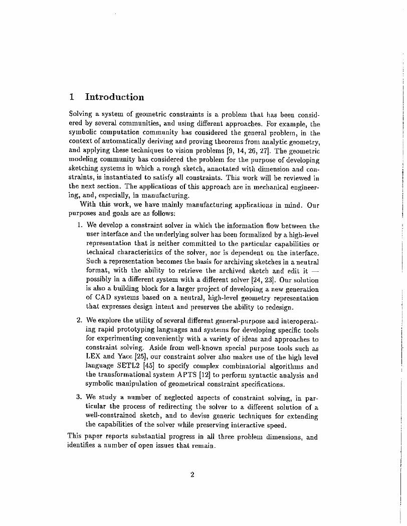
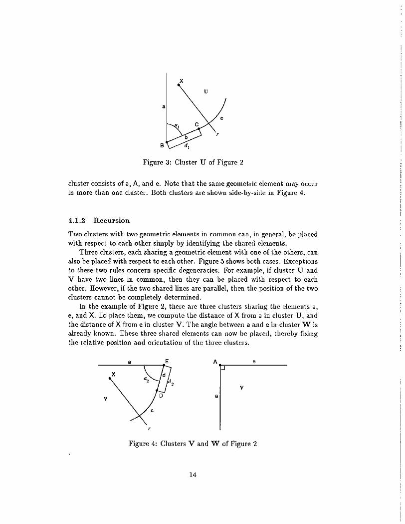
For example, in the graph of FIgure ·2, we may begin with elements a and B,effectively drawlng a line a and placing on it the point B anywhere. We cannow place in sequence b, C, and X. At thls point, no additional elements can beplaced and the cluster is complete, as shown In Figure 3. Note that we neitherknow where A is situated, nor how far the arc c extends. Starting agaill, twoother clusters are determined. One consists of X, D, d, E, and e. The other

13

xu

a

c

b

B d,

c,

Figure 3: Cluster U of Figure 2

cluster consists of a, A, and e. Note that the same geometrir. element lllay occurin more than one cluster. Both clusters aTe shown side-by-side in Figure 4.

4.1.2 Recursion

Two clusters with two geometric elements ill common can, ill ,!?;f'lleral, hI" placedwith respect to each other simllly by identifying the shared elements.

Three clusters, each sharing a geometrlc element with one of the others, canalso be placed with respect to each other. Figure 5 shows both cases. Exceptionsto these two rules concern specific degeneracies. For example, if cluster U andV have two lines in common, then they can be placed with respect to eachother. However, if the two shared lines are parallel, then the position of the twoclusters cannot be completely determined.

In the example of Figure 2, there are three clusters sh,Lring the elements a,e, and X. To place them, we compute the distance of X from a in cluster U, andthe distance of X from e in cluster V. The angle between a and e in cluster W isalready known. These three shared elements can now be placed, thereby fIxingthe relative position and orientation of the three clusters.

v

x

,

,

A .-~,---__--"' _

va

Figure 4: Clusters V and W of Figure 2

14

u

•v

Figure .5: Recursive Cluster Placelllfmt

The two cluster placement rules conceptually build a larger cluster from twoor three smaller ones. Additional clusters sharing two elements with this new"super cluster" can be added in the same way, thereby growing larger clustersfrom smaller ones. Recursively, super clusters can be placed witl] respect toeach other in the same way.

4.1.3 Construction Steps

The reduction steps correspond to standardized geometric construction steps,and also to solving standardized, small systems of algebraic equations. Theconstruction steps include the following:

Basis Steps: The basis steps place two geometric elements related by agraph edge. They include placing a point on a line, v1acing two lines at a givenangle, placing two points at a given distance, and so on. Note that in generalthere are several ways to place the geometric element.

Point Placements: These rules place a point using two constraints. Theyinclude placing a point at prescribed distance from two given points, or atprescribed distances from given lines, and so on. See also Figure 6.

Line Placements: These rules place a line with respect to two given geo­metric elements. They include placing a line tangent to a circle through a givenpoint, at given distance from two points, etc.

Circle Placement: These rules place a circle of fixed or variable radius.Fixed-radius circles require only two constraints and determining them can bereduced to placing the center point. Variable-radius circles require three con­straints and reduce in many cases to the Apollonius problem - fincling a circlethat is tangent to three given ones.

Cluster' Placement; Clusters are placed by placing; shared geometries. ITnecessary, the relationship between the shared geometric elements is computedwithin each cluster, whereupon the two or three shared elements can be placed

15

./ r

.:.0:;:>'. .

(/"::\"j\·····..l!.·····/

.'...........'

•

·".""".........

//

Figure 6: Point Placement Rules: Left, by Distance from Two Points; Right,by Distance from Two Lines.

with respect to each other.Algebraic Fommlation: Geometric elements are represented as follows: Points

are represented by Cartesian coordinates. A line is determined from its implicitequation in which the coefficients have heen normalized:

a: mx+ny+p=O

It is well-known that in this formulation p is the distaIlC,C'. of the origin [rom theline. Because of the normalization, lines are determined only IJy two numericalquantities, the (signed) distance p of the origin from the line, and the directionangle cos 0: = n. Therefore, two constraints determine a line. Lines are orientedby choosing (-n, m) as the direction of tIle line. Circles are represented by theCartesian coordinates of the center and the radius, an nnsigned number.

In many cases it is quite obvious how to determine the worclinates of thenext geometric element from tlle constraints relating it to known geometricelements. By restricting to simple construction steps, the basic algorithm solvesat most quadratic equations. In some cases, up to three simultaneous quadraticequations must be solved. For example, given three circles of fixed radius,finding a circle tangent to all three requires solving the foUowiug system,

(x - x,)' + (y - y,)'

(x - X2)2 + (y - Y2r =

(x - x,)' + (y - y,)'

(,. ± ",)'(, ± ,.,)'(,. ± ,,)'

where the choice of the sign on the right-hand sides determines which of up toeight possilJle solutions is determined. Here, (XI:,YI:) is the eenter ofcirde k, and1'1: is its radius. Such constructions are done by precomputin?; a normal form ofthe system from which to the unknowns are easier to filld. Preprocessing canbe done using Grabner bases; e.g., [8].

16

A•

c•

A----'--o

.----,--c

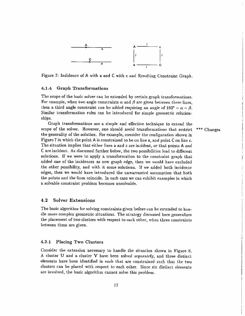
Figure 7: lndiclence of A with a and C with c and Resulting Constraint Graph.

4.1.4 Graph Transformations

The scope of the basic solver can be extended by certain ~raph transformations.For example, when two angle constraints Q and [3 are given between tlm.'C' lines,then a third angle constraint can be added requiring an angle of 1800

- Q -[3.Similar transformation rules can be introduced for simple geometric relation­ships.

Graph transformations are a simple and effective technique to extend thescope of the solver. However, one should avoid transformations that restrict *** Changesthe generality of the solution. For example, consider the configuration shown inFigure 7 in which the point A is constrained to be on line a, and point C olllille c.The situation implies that either lines a and c are incident, or that l)Qints A andCare incidellt. As discussed further below, the two possibilities lead to differentsolutions. IT we were to apply a transformation to the constraint graph thatadded one of the incidences as new graph edge, then we would have excludedthe other possil)ility, and with it some solutions. If we added both incidenceedges, then we would have introduced the unwarranted assumption that boththe points and the lines coincide. In each CMe we can exhibit examples in whicha solvable constraillt problem l)ecomes unsolvable.

4.2 Solver Extensions

The basic algorithm for solving constraillts givon before GLll l)e extended to han­(lie more complex geometric situations. The strategy disc-lIssed here generalizesthe placement of two clusters with respect to each other, when three constraintsbetween them are given.

4.2.1 Placing Two Clusters

Consider the extension necessary to hamUl'. the situation shown in Fip;ure 8.A cluster U and a cluster V have been solved separatdy, and three distinctelements have been identified in each that are COIlS trained such that the twoclusters call be placed with respect to each other. Since six (Ustinct elementsare involved, the basic algorithm cannot solve this problem.

17

A dJi a

d alp'

dJi B dJi b dfi

dJi dJidJi

U c C

V

Figure 8, Case (p,p,l) =" (l,I,p)

If we examine every possible configuration of two clusters so related by threeconstraints and add graph reductions that place such clusters with respect toeach other, then the solver has been extended to a much lar~er class of con­straint problems. We analyze one constraint configuration. In this particularconfiguration, as well as in a uuml)er of other cases, the solver's competence isextended beyond ruler-and-compass constructible configurations.

Assume that in cluster U the three elements are the points A and Bandthe line c, and in cluster V the elements aTC two lines a and b and a llOinlC. The constraint possibilities aTe d for distance, i for incidence, (L for angle,and p for parallel. Depending on the combination of these constraint types, aconstruction sequence can be determined that fixes one cluster with respect tothe other.

In the configuration considered, it is advantageous to fix duster V and lllovecluster U relative to it such that all constraints are satisfied. Conceptually, wesolve the cases in one of two ways:

(AJ For some combinations, a sequence of ordinary construction steps placesthe second cluster, possil)ly with the introduction of auxiliary constructionpoints, lines and/or circles.

(BJ For some combinations, we consider two of the three constraints and pre­compute the locus of tbe geometric element whose collstraint has beenignored for the moment. If this element is a point, the locus is an implicitalgebraic curve whose coefficients are expressions in the given constraints.Then, the precomputed locus is intersected with a construction line orcircle and the intersections identify those positions for the third geollletricelement for which all constraints are satisfied.

Note that the second method is not necessarily equivalent to a ruler-and-compassconstruction.

IS

Subcase Properties Properties Constrain ts Method of

Number olU olY Combination Solution

Aic Cia A i a

1. B dji c C dji b B dji b (A)

AdB a alp b ciC

Ai c Cd a Aia

2. B dji c Cd b B dji b (B)

AdB a alp b c i C

Ad c Cia A i a

3. B de Cd b B dji b (B)

AdB a ajp b ciC

Table 1: Essential Combinations of(p,p,l)= (I,l,p). Constraint symbols arei = incident, d = nonzero distance, p = parallel, a = nonzero (ltlg-Ie.

Table 1 sumlllarizes the essential cOllll)inations and identifies which approachis to be used. The other combinations can be mapped to those of the table byreplacing some of the lines in U and V with suitably positionp.d parallel lines.

Consider Subcase 1, assuming that B is not incident to c, and that B shouldbe at distance e from b. The two clusters are shown in Figure 9, with T tllC'distance of A from Band t the distance of B from c. Two families of solutionsexist: Either the lines a and c coincide, possibly in oppo:>ite orientation, orthe points A and C coinci(le. In the first situation, the locus of B is a p,ur oflines parallel to c, at distance t. Four intersections with lines parallel to b atdistance e are four possible locations for B, and each of til em determines therelative llOsition of U with respect to V. In the second situation, the locus of B1s a circle aTOund A, and the up to four intersections with lines parallel to b atdistance e are the possible locations for B.

Now consider Subcase 2 in Table 1. We determine the C'.llrve that is the locusof B, assuming that B has coordinates (x, y). By a eoordinate transformation,

c

a

b

Figure 9: Suhcase 1 Configuration

19

'-~~." "

"~~

, , ,, ,

"

A C, ,

'.'"

""

"-------------------------------------~----­'"

b

Figure 10: Subcase 1, First Solution

b

"

",

---"

" "

"

""

,,

".~ /~

, ,"'~.,,,,,,,,,

:--------"'o-------'-':'~"'--"''''',-'-'-''-'"'''--, .~~ ~~~~, A,C ' •, ,, ,, ,\ r ;

,,,,/-'

Figure 11: Subcase 1, Second Solution

20

,

8

C.. (O,l)

,

Figure 12: Case 8 d c, A i c

moreover, we can assume that C has coordinates (0,1) and that A, constrainedto he on a, has coordinates (a, D). [n the simplest case, A and B are both on c,distance dj apart. In Figure 12 this wrrcsponds to d2 = O.

The cotangent of the angle 8 between lines c and a is then -a, so th;:L1 wecan express sin () = lin and cosO = -a/n, where u = VI + a2

• The locus of Bcan therefore be described by three equations:

xu-au+d1a 0

yu - d] 0

u 2 _ a2 I

Eliminating a with a Grabner basis computation establishes that the locus of Bis the degree 4 curve

If d2 ::j:. 0; i.e., if B does not lie on C, then the equations describing the locus ofB are only slightly more complicated, and are

xu- au+d1u+d2 0

Ylt - d] +d2u 0u 2 _ a2 1

Again, B lies all a degree 01 curve whose coefficiellts ar~ polynomial in (II and d2

of degree 4.The most general situation occurs when A is not on c, as shown in Figure 13.

Other cases can be reduced to this sitnation by replacing the lines with parallellines at a suitable distance. Referring to Figure 13, the equations describing the

21

B

,

A~(a.o:)",.L-7''-c= -:cA'~(a',O) a

Figure 1;3: Case B dc, A d c

locus of Barexu - au +dIa' + do - d2 0

yu - d} + doa' - d2 (L' 0

a - a' + dou 0u 2 _ at2 I

By a Grabner basis computation one determines that the locus of 8 is also acurve of degree 4. The coefficients are polynomials in the dk of degree up to 4.

Many other combinations of three constraints between two clusters must beconsidered when so extending the solver. In each case, we conceptually satisfytwo constraints and examine the locus of the geometric item whose constraint weignored under the remaining degree offreedom. Thus, it suffices to examlne pairsof constraints between two clusters and derive, for each arising case, the locusof the element in question. Since we have the c1lOice of which two constraintsto satisfy, the number of different cases can be reduced significalltly.

IT the element whose locus we determine 1s not a llOint, then we need equa­tions for the determining quantities. In the case of lines, those are the coefficientsof the line equation, or, equ.ivalently, the direction angle and the distance fromthe origin. For example, consider the case (p, I, l) == (l, p, l). Here we lllay wantto avproach the situation as we did in the case (p,l,l) == (l,p,p), and precom­pute how the line equation varies w1th the remaining mobility when satisfyingthe first two constraints. In the subcase 3, the most general situation, we haveto determine the distance of the moving line from the origin and the componentsof the normal vector after norming it to length 1; see also Figure 14. Let a bethe fixed angle between the lines band c, 8 the angle determining a particularposition ofthe moving configurat1on. Let i be the direction angle of a line d wlthwhich b is to form an angle 6. Then we mllst solve a±8 = i±6, accounting forthe d1fferent vositions of the moving configuration in which the constraints canbe satisfied. Once 8 is known, the resulting configuration is easily computed. Inmore complicated sltuat1ons, a system of equations is formulated as for the point

22

"

d, C=(O,1)

A=(a,O) , ,A'={a',O) D, a

d"

b

Figure l4: Configuration for Satisfying Line Constraints

locus, expressing line distance from the origin and direction angle as fUlldionof the parameters and an additional quantity, such as () or the coordinates of amoving point, and a nonlinear equation is solved that is precomputed from thesystem using Grabner bases.

Ultimately, many of the cases and subcases we have to consider reduce toa few generic situations that are characterized by the selection of which twoof the three constraints govern the relative motion between the two dusters.Particularly in the case of point loci, classical curves aTe obtained that aredescribed in the literature; see, e.g., [a6], or the literature on plane kinematics.The curve of subcase 2 above, with d2 = 0, is a conchoi([ of a line. In Figure15 a segment end is constrained to a circle and the sc,!!;tl1cn t incident to a fixedperimeter point C. This case is solved by the limacon oj Pascal, a c-onchoj<] ofthe circle.

Bc

A

Figure 15: Locus of Segment Through a Fixed Perimeter Point is the Limaconof Pascal

2;j

",,,

sp:o,,-..,;

40.0

Figure 16: Several Structurally Distinct Solutions of the Same Constraint Prob­lem

5 User Interaction

In general, a well-constrained geometric constraint problem has an exponentialnumber of solutions. For example, consider drawing n points, along with 2n - 3distance constraints between them, and assume that the distance constraints aresuch that we can place the points serially, each time determining the next pointby two distances from two known points. In general, each new }lOint can 118placed in two different locations: Let Po and PI be known points from which thenew point q is to be put at distance do and d[, respectively. Draw two circles, oneabout Po with radius do, the other about PI> with radius d\o The intersectionof the two circles are the possible locations of q. For n points, therefore, wecould have up to 2"-2 solutions. Which of these solutions is the intended onewould depend on the application that created the constraint problem in thefirst place. We discuss how one might select the "right" solution. We callthis the root identification problem, because on a technical level it correspondsto selecting one among a number of different roots of a system of nonlinearalgebraic equations.

Although some solutions of a well constrained problem are merely symmetricarrangements of the same shape, others may differ strllctnrally a great deal.Figure 16 shows several possibilities to illustrate the possihle range. But anapplication will usually requ.ire one specific solution. To identify the intendedsolution is not always a trivial undertaking. Moreover, the wide range of llossiblesolutions has severe consequences on the problem of communicating a genericdesign based on well-constrained sketches. Since a sketch with a constraintschema would not necessarily identify which solution is the intended one, moreneeds to be communicated.

In tltis section, we consider three approaches: selectively moving geomet­ric elements, adding more constraints to narrow down the number of possiblesolutions, and, finally, a dialogue with the constraint solver that identifies inter­actively the intended solution. These aTe approaches that have to contend withsome difficult technical problems. We also consider the llossibility of structuring

24

the constraint problem hierarchically. Doing so would increase knowledge of thedesign intent, and would diminish some of the mOl'e obviolls technical problems.

5.1 Moving Selected Geometric Elements

All constraint solvers known to us adopt a set of rules by which to selec.t thesolution that is ultimately presented to the user. Whether slated explicilly, aswe will later, or incorporated implicitly into the code of the solver, these rulesultimately infer which solution would be meant by observing topological and/orcoordinate relationships of the initial sketch with which the user specified theconstraint problem, When the solution is presented graphically to the user, itseems natural that the user, again graphically, select certain geometric elementsof the final sketch that are considered misplaced. The USCI' could then showthe solver where the selected element(s) should be placed in fplation to otherelements by moving them with the mouse.

This very simple idea ultimately may be effective, Imt there are a numberof conceptual difficulties that need to be overcome. For example, picking it

geometric element is ambiguous. Because of the recursive nature of the solver,picking could refer to the individual clement, or to the cluster or super cluslersof which it became part. MOTe importantly, the required restructuring mightentail more complex operations than merely moving a single ~roup of geometricelements. Furthermore, since the length of segments and arcs often implicitlydepends on the final placement, it is not clear whether lhe user can reasonablybe expec.ted to understand the effect of moving geometriC's.

In DeM [19, 38]' a moue instruction relocates a g:(,01llctrir ('lement. There­upon, the solution can be recomputed, and other elements can be moved. itappears that the solver uses the new position coordinates when applying: thenormal placement heuristics selecting a solution. We found the move instruc­tion difficult. Some of the time, the effect was as intended, hul lllany times itwas unexpected. However, with more research, a useful paradig:m for identifyingintended solutions of geometric constraint problems may well cmerg:e.

5.2 Adding More Constraints

Consider once more the problem of placing n points with presnibed distances.We could narrow down which solution is meant in one of two ways: We may adddomain knowledge from the application, or we ma.y give a.d(litional geometricconstraints that actually overconstrain the problem. Unfortunately, both ideasresult in NP-complete problems.

For instance, assume that the set of points is the set of verlices of a polygonalcross section. In that case, application-specific information might require that

25

d,

Figure 17: Two Solutions for Three Parallel Lines

the resulting cross section is a simple polygon; that is, it should form a polygonthat is not self-intersecting. This may be COlllllllLtUcated by giving, in addHion,a cyclical ordering of the points; i.e., the sequence of vertices of the cross section.This very simT)le additional requirement makes the problem NP-complete:

Theorem (Capoyleas)Given n llOints in the plane that are well-constrained by 2n - 3point-to-point distances, and a cyclical ordering specifying how toconnect the points to obtain a polygon. Then identifying a solutionfor which the resulting polygon is simple, i.e., is not self-intersecting,is NP-complete.

Consequently, there is little hope for adding domain-specific knowledge aboutthe application with the expectation of obtaining an efficient constraint solverthat finds the intended solution in all cases.

Instead of adding application-specific rules, for instance to derive simplepolygons, we could add more geometric constraints. For e-xample, considerspecifying three parallel lines along with distances between two pairs of them.As shown in Figure 17, there are two dlstinct solutions of tltis well-constrainedproblem. By adding a required distance between the thir<1 pair of parallel lineswe can eliminate one or tlle other case, and make the solution llluql1e.

Overconstrained geometric problems have been carefully avoided by th(l. fieldbecause the set of constraints might be contradictory. However, blue printsare usually overdimensioned, although not for reasons of eliminating unwantedsolutions, but for limiting errors through redundancy. Again, it is unfortunatethat even for the simple case of placing parallel lines the overconstrained problemis NP-complete.

Since adding constraints even in such simple situations results in NP-completeproblems, it seems to us that the attractive idea of adcling more constraints tonarrow the range of possible solutions will not work very well in practice. It islllallsible that a heuristic approac11 succeeds in solving this problem in a rangeof cases that are of practical interest, but always with the possibility that forspecific instances the solver would bog down. Again, further research is neede(1to better understalld the potentialities of the approach.

26

5.3 Dialogue with the Solver

The considerations above seem to suggest that no automatic <tvproach to rootidentification will succeed in delivering an efficient constraint solver that gets theintended solution every time. Conscqucntly, we feel tllat a promising alternativeis to devise a few simple heuristics that succeed in many cases and are easy tounderstand. Beyond that, we rely on interaction with the user in those cases inwhich the heuristics fail to deliver an acceptable solution. Note that placementrules are used very widely, but are rarely discussed.

5.3.1 Placement Heuristics

All solvers known to us derive from the initial g-eolllf'trir sketch informationthat is used to select a specific solution. This is reasonable, since ont>o canexpect that a sketch is at least topologically accurate, so that obscrving onwhich side of an oriented line a specific point lies in the sketc.h is often reliablyindicating where it should be in the final solution. HowevPf, when genericdesigns are archived and and later edited, one should no longer expect suchsimple correspondences between the sketch and the ultimate solution, becauseas dimension values change, so may the side ofa line on which a voint is situate<!.

In our system, we use very few but highly effective rules. We keep the numberof rules to a minimum because we do not believe that mot idelltific.ation has asatisfactory and completely automated solution. Where the rules fail, we relyon user interaction to amend them M the situation might requ.ire. Note that ourrules are fully supported by the Erep approaclI in that the different situationscan be characterized and recorded faithfully.

Three Points: Consider placing three points, PI, P2 and ]13, relative to eachother. The points have been drawn in the initial sketch in some position, andtherefore have an order that is determined as follows. Determine where P3 lieswith respect to the line (PilP2) oriented from PI to P2. If ]);1 is on the line, thcndetermine whether it lies between PI alld P2, preceding 1)1 or following P2' Thesolver will preserve this orientation if possible.

Two Lines and One Point: When placing a point relativt' to two lines, oneof four possible locations is selected based on the {Juadrallt of the oriented lint'sin which the point lies in the original sketch. Note that tbe line orientationpermits an unambiguous specification of the angle between the lines.

One Line and Two Points: The line is oriented, and the points, PI andP2, are kept on the same side(s) of the line as they were ill the original skel.ch.Furthermore, we preserve the orientation of the vector PI' P2 with respect to theline orientation by preserving the sign of the inner product with the line tangentvector.

Tangent A1'C: An arc tangent to two lille segments will he centered such that

27

~_..Figure 18: The Two Types of Tangency lletween an ArC'. and a Segment

the arc subLended preserves the type of tangency. The two types of tangencyaTe illustrated in Figure 18. Moreover, the center will be placed such that thesmaller of the two arcs possihle is chosen, ties broken hy lllacing the center OIl

the same side of the two segments as in the illput sketch. As specific degeneracyheuristics, an arc oflength 00 is suppressed.

All rules except the tangency rule are mutually exclusive. They are thereforeapplicable without interference. The tangency rule could contradict the otherrules, because dimensioned arcs and circles are determined l>y placing lhe center.In such cases, the tangency rule takes precedence. In aliI' experiments with thE'serules, we found that most situations are solved as the user would exped. Therules arc easy to implement, and are easy to un(lerstand for the user.

5.3.2 Selecting Alternative Solutions

A useful paradigm for user-solver interaction has to be intuitive and must ac­count for the fact that most application users will not (and sllOuld not) be inti­mately knowledgeable about the technical workings of t1](' solver. So, we needa simple but effective communication paradigm by which the user can interactwith the solver and direct it to a different solution, or even browse through asubset of solutions in case the one that was found is not "right."

Conceptually, aU possible solutions of a constraint problem can he arrangedin a tree whose leaves are the different solutions, and whose internal nodescorrespond to stages in the placement of elements or dl1sters. The differentbranches from a particular node are the different choices for placing the elementor duster. The tree has depth proportional to the number of elements andclusters. Browsing through all possible solutions would be'! exponential in thenumber of elements and would be illaptlTopriate, but steppinj?; from one solutionto another one is proportional to the tree depth only.

We have added to our solver an incremental mode in which the user canbrowse through the. construction tree amI be visually infoTluE'.d whieh ele.menlshave been placed at a particular moment. "Vith a buttOll, thp user steps forwardor backwards in the construction sequence, thus traversing the tree patll back­wards, towards the root, or forward, towards a leaf. At each level, the geometricelement(s) placed at that point are highlighted, and a panel displays the lHlluherof possihle positions. The user can then select which aIle of the ]Jossihle choices

28

should be used.For example, consider the constraint example of Figure 2. TIle role of the arc

is clearly to round the corner that would be formed otherwise by the adjacentsegments. When drawn as indicated in the figure, and with an,!:!;le values largerthan 45°, the solver finds the leftmost solution in Fignre 16. However, whenthe angles are changed subsequently to 30°, the solver hellristics will select thp.solution shown in Figure 19, llecause the center of the arc remains on the sameside of the adjaccnt segments. The user now relocates the center by chan~ill?;

Figure 19: Default Solution After Changing Angles

the placement of ArlO with respect to 897 and 899- By pressing the levelImttons, the user returns to level 7. Here, ArlO and 897 are highlighted. Theuser now changes the solution by prpssing the 801n. buttons. This chauges thearc center with respect to 897 only. Continuing with the level buttons, on level4 AriD and 899 are highlighted. Again, a different solution is selected on thatlevel, changing the arc with respect to 899. Now the solver will construd thesolution shown in Figure 20. We have found this simple interaction techniquehighly useful in exploring alternative solutions, and most users become effectivein directing the solution process in a very short time.

In the Erep specifications of the interaction process, the solver is instructedserially to perform a back-up or to seek the next way to place an element or acluster. This convention excludes solvers that find a solution lly a numerical,iterative computation which places all geometric clements at once, unless the it-

29

P12~

90.000 Sg5

Figure 20: Interactively Changing Solutions: Elements hi?;hlighted are placedwith respect to each other at this level in the solution tree.

30

I 72.0

r 60.0

72.0

L60.0 20.0

Figure 21: A Constraint Problem

eration is based on homotopy contitlllation techniques th,tL can find all solutionsof a nonlinear system of equations numerically.

Note that different solvers liay cluster geometric elements differently andplace the elements and clusters in a different sequence. Therefore, the sameinteraction sequence with the solver would have different effects witl\ dlfferenLsolving algorithms. This cannot be avoided: To arrange' thp tree of solutions illcanonical order, we either prescribe a canonical sequence a-pl'im'i in which thegeometric elements have to be computed, or else we compute a canonicallmsisfor the ideal generated by the constraint equations that describe the geometricproblem, and then enumerate the associated variety in a canonical way; e.g., [8].m the first case, we would prescribe the solver algorithm to llelong to a certainfamily. In the second case, the ideal basis computation is equivalent to solvingthe constraint problem and thus constitutes committing to a canonical solver. 1T

Both ways compromise devising a neutral format of archiving. Consequently,we can neutrally archive a constraint problem (solved or ullsolvNI), but not themanner in which to solve or seek an alternative solution. This is an intrinsicproblem when solving geometric constraints.

5.4 Design Paradigm Approach

Consider solving the constraint problem of Figure 21. TIl(' role of the arc isclearly to round the adjacent segments, and thus it is most likely that thesolution shown in Figure 22 on the left is the one the user meant rather than theone on the right, when changing the angles to 30°. The solver would be unawmeof the intended meaning of the are, a.lld thus needs a. tf'chnical heuristic , suchas the tangent arc rule, to avoid the solution on the right. It would bl" Illllchsimpler if the user would sketch in such a way that the dc-sigll intent of the arcis evident.

IIBeca.llse SUdl a canonical solver would be completely general, il could not be very fa.~t illma.ny situations, since tile efficiency of constraint solvers rests Oil r~trieting the generality ofthe solver.

31

r 20.0

Tv

75.0

30.0 30.0

20.0

TvFigure 22: Two Solutions of the Constraint Problem of Figure 21 after ChangingAngles

The difficulty for the geometric constraint solver is that sketches aTe usuallyflat; i,e., the geometric elements are not grouped into "features." It would bebetter to make sketches hierarchically: First, a basic dimension-driven sketchwould be given. Then, subsequent steps, also dimension-driven, would modifythe basic sketch and add complexity. In our example, the bcu;ic sketch couldbe a quadrilateral. There would be one subsequent modification adding a two­dimensional 7YJund with a required radius. This is analogous to feature-baseddesign a.'> implemented in current CAD systems.

The hierarchical approach to sketching has other important benefits. Sincethe sketch is structured, later modifications can be driven [rom constraints usp.din earlier steps, so that simple functional dependencies and relations betweendimension variables of previously defined sketch features can be defined andilll}llemented with trivial extensions of our basic constraint. solver.

6 Summary and Future Work

Researc1l on constraint solving should develop natural paradij:!;llls for narrowingdown the number of llOssibie solutions of a well-constrained geometric prolllemand devising solver interaction paradigms that allow the user to corred solutionsthat were not intended. With increasing penetration of constraint-based designinterfaces, this prolliem is becoming increasingly mon~ pressing.

Which solution is the intended one is also an issne when considering designarchival in a neutral format. So far, neutral archiving formal.s have been re­stricted to detailed design without a formal record of design intent, constraintschema, editing hancUes, and so on. Where editable design has been archived,it has been done in a proprietary format native to tlle particular CAD system,and is typically a record of the internal data structures of the CAD system. In[24] we have presented alternatives. Current trends in data exchange standardsindicate a growing interest in archiving constraint-based designs in which tItis

32

additional information has been formalized without commitment to a particularCAD system.

In constraint-based, feature-based design, it is common to have available- avariational constraint solver for 2D constraint problems, hut not for ;lD geo­metric constraints. This is particularly apparent in the pCl'si..dent id p7'Oblemdiscussed in [23]. A well-conceived 3D constraint solver cOlH:eivalJly can avoidthese problems and assist in devising graphical techniCJues for generic design.

III manufacturing applications one is interested in functional relationshipsbetween dimension variables, because such relationships can express design in­tent very flexibly. Some parametric relationships can be implemented easily bystrncturing the sketcher as advocated in Section 5.4. Moreover, simple func­tional relationships are the content of certain geometry theorems, such as thetheorems of proportionality, and many other c1a.'isical resulls. Such theoremscan l)e added to the constraint solver in a mamler analo/1;olls to the extensionswe have discussed before. But in general, functional relationships between di­mension variables necessitate additional mathematical techni{IUes. Geometrictheorem proving has developed many general techniques that are applicable,but suitable restrictions are still needed to achieve higher solver speeds.

Geometric coverage refers to the range of shapes the constraint solver un­derstands. In this work, we have restricted the geometric coverage to points.lines and circles. Conic sections would be easy to add, as would be splines suchas Bezier curves, when translating the constraints to equivalent ones on controlpoints. There is a rich repertoire of literature in CAG D that provides convenienttools for doing so. Yet it is far from clear whether control point manipulationsare a universal tool for expressing constraints tllat the llser finds natural, andwe miss stu{lies that analyze how to design with splillPS from all application'spoint of view.

Even with the restided geometric coverage discussed here, some theoreticalproblems remain open. Althongh no IJrecise analysis has been made, neitherOwen's nor our constraint solving algorithm seems to run in worst case timelinear in the number of graph edges. We conjecture that both algorithms run inquadratic time due to repeated traversals over regions of the graph. It would beworthwhile to analyze the worst case running times of these algorithms precisely,and study how to improve it. It is also worthwhile to consid{'r how to minimizethe arithmetic operations involved in the constructiou steps, and to analyzeconstruction sequences for numerical stability.

Acknowledgement

We had several insightful discussions with John Owen from D-Cubed, Ltd.

33

References

[1] B. Aldefeld. Variation of geometries based on a ,!'!;c'ometric-reasoningmethod. G'ompuic7' Aided Design, 20(3): 117-126, April 1988.

[2] L. A. Barlord. A Gmphical, Language-Based Editol' /01" Generic Solid Mod·cl.~ Represented by Constminls. PhD thesis, DC'pt of Computer Science,Cornell University, March 1987. TR 87-813.

[;3] A. H. Barning. The programming langua,!!;e aspects of ThingLab, a COll­

straint oriented simulation laboratory. AeM TOPLA 8, 3(4):353-387, 1981.

[4] P. Borras, D. Clement, T. Despeyroux, J. Incerpi, G. Kahn, B. Lang, andV. Pascual. Centaur: the system. Technical Report Rapports de Recherche777, INRlA, 1987.

[5] D. H. Brown Associates. Conceptual Design: Tradeolfs in PerfOl'mance andFlexibility. Notes on the design of Pro/ENGINEER, Hl91.

[6J B. Brllderlin. Constructing Thee-Dimensional Geometric Objects Definedby Constraints. In Workshop on Intemctive 3D Graphics, pages 111-129.ACM, October 23-24 Hl86.

[7J B. Buchberger. Ein Algorithmus zum Auffinden del' Basiselcmente desRcslklassenringes nach einem nttlldimensionalen Polynomideal. PhD the­sis, University of Innsbruck, Austria, 1965.

[8] B. Buchberger. Grabner Bases: An Algorithmic Method in PolynomialIdeal Theory. In N. K. Bose, editor, M1tltidimcll.~ional Systems Theory,pages 184-232. D. Reidel Publishing Co., 1985.

[9] B. Buchberger, G. Collins, and B. Kutzler. Algebraic methods [or geometricreasoning. Annual Retliews in Computel' Science, 3:85-120, 1988.

[10J A. Bundy and R. Welham. Using Meta-level Inference for Selective Appli­cation of Multiple Rewrite Rule Sets in Algebraic Manipulation. Al'tijicialIntelligence, 16:189-212, 1981.

[11] J. Cal. A language fOT semantic analysis. Technical Report 635, New YOTkUniversity, Dept. of Camp. Science, 1993.

[12] J. Cai, P. Facon, F. Henglein, R. Paige, and E. Schonberg. Type trans­formation and data structure choice. In B. MoeUcr, ('clitOT, COllsll'uctingProymms From Specijicatio7l.':;, pages 126-124. North-Holland, 1991.

[13J J. Ca.i and R. Paige. Towards increased productivity of algorithm imple­mentation. ACM SIGSOFT, to appear, 199;3.

34

[14] C.-S. Chou. Mechanical Theorem Proving. D. Reidel Publishing, Dordrecht,1987.

[15] C.-S. Chon. A Method for the Mechanical Derivation of Formulas in BIt:!·mentary Geometry. Jov.mal of Automated Reasoning, :3:291-299, Hl87.

[16] C.-S. Chou. An Introduction to Wn's Method for Mechanical TheoremProving in Geometry. Jom'nal oj Automated Reasoning, 4:237-267,1988.

[17] C.-S. Chou and W. Schelter. Proving Geometry Theorems with RewriteRules. Joumal of Automated Reasoning, 2:253-273, 19R6.

[18] W. Clocksin and C. Mellish. Pmgramming in Pm/og. Springer Verhtg, 1981.

[19] D·Cuhed Ltd, 68 Castle Street, Cambridge, CB3 OA.J, England. The Di­mensional Constmint Manager', May 1993. Versioll 2.5.

[20] W. Fitzgerald. Using Axial Dimensions to Determine the Proportions ofLine Drawings in Computer Graphics. Computel' Aided Design, 13(6):377­382, November 1981.

[21] B. Freeman-Benson, J. Maloney, and A. Borning. An Incremental Con­straint Solver. CACM, 33(1):54-63,1990.

[22] J. Gosling. Algebraic Constraints. Technical Report CMU-CS-R3-132,eMU, 1983.

[2:3] C. M. Hoffmann. On the semantics of generative geometry rcprC'sentations.In 19th A5'ME Design Automation Conference, 199;3.

[24] C. M. Hoffmann and R. Juan. Erep, a editable, high-IevC'!l representationfor geometric design and analysis. In P. Wilson, M. Wozny, and M. Pratt,editors, Geometric and Pmducl Modeling. North Holland, 1993.

[25] S. Johnson. Yacc - yet another compiler compiler. Tec1mical Report Com·puter Science Report 32, AT&T Bell Laboratories, Murray Hill, N.J., 1975.

[26J D. Kapur. A rcfutatiollal approach to geometry theorem proving. InD. Kapur and J. Mundy, editors, Geometlic Rcm:oning, pages 61-93. M.LT.Press, 1989.

[27] D. Kapur and J. Mundy. Wu's method and its applications to perspectiveviewing. In D. Kapur and J. Mundy, editors, Gcomctlic Reasoning, pages15-36. M.LT. Press, 1988.

[28] D. Knuth. Semantics of context-free languages. lv/athematical SystemsTheory, 2:127-145, 1968.

35

[29] D. Knutll and P. Bendix, Simple word problems in universal algebras. InJ. Leech, editor, Computational P1'Obiems in Ab.~tmct Algebm, pages 263­297. Pergammon Press, Oxford, 1970.

[30J K. Kondo. PIGMOD: parametric and interactive geometric 1llodeller formechanical design. Computer Aided Design, 22(10):6;3;3-644, December1990.

[31] K. Kondo. Algebraic method for manipulation of dimensional relationshipsin geometric models. Compute1' Aided Design, 24(;3):141-11\7, March 1992.

[32] G. Kramer. Solving G'eometr7:c G'onstmint Sy.~tems. MIT Press, 1992.

[33J W. LeIer. Conslmint Frogmmming Languages: Theil' Specification andG'enemtion. Addison Wesley, 1988.

[34J J. Li. Using algebraic constraints in interactive text and graph.ics editing.In D. A. Duce and P. Jancene, editors, EU1'Ogmphies '88, pages 197-20.5.Elsevier North-Holland, 1988.

[35J R. Light and D. Gossard. Modification of geometric models through vari­ational geometry. Computel' Aided Design, 14:209-214, .July 1982.

[36] E. H. Lockwood. A Book oj CUl"es. Cambridge University Press, 1961.

[37] G. Nelson. Juno, a costraint-based graphics system. In SIGGRAPH, llages235-243, San Fratlcisco, July 22-26 1985, ACM.

[38J J. Owen. Algebraic solution for geometry from dimensional constraints. InACM Symp. Found. oj Solid Modeling, pages 397-407, Austin, Tex, 1991.

[39J R. Paige. Apts external specification manual. internal documentation,1993.

[1\ OJ Pro/ENGINEER. Modeling Use",,; Guide: 2D Skctchcl'. ParametriC'Tech­nologies. Release 8.0.

[41J Reasonlng Systems. Refine User's Guide, 1990. Version :}.O.

[42] T. Reps and T. Teitelbaum. The 8ynthsizC1' Generat01·. Springer Verlag,1988.

[43] A. Requicha. Dimensionlning and tolerancinp;. Technical report, ProductionAutomation Project, University of Rochester, May 1977. PADLTM-19.

(44) J. Schwartz, R. Dewar, D. Dubinsky, and E. Schonberg, Pmgrammillg withSets: Au iutmduction to SET£. Springer Verlag, 1986.

36

[4,s] K. Snyder. The SETL2 programming languag~. Technical rcport, NewYork University, Computer Scicnce, Couranl Institute, 1990.

[46] W. Sohrt. Interaction with Constraints ill three-dimensional Modeling.Master's thesis, Dept of Computer Science, The University of Utah, March1991.

[47] L. Solano and P. Brunet. A system for constructive cOIlstl'aint-based model­ing. In B. Falcidieno and T. Kunii, editors, Modeling in Computcl· Gmphics.Springer Verlag, 1993.

(48] G. 1. Steele and G. 1. Sussman. CONSTRAINTS - A Language for Ex­pressing Almost-Hierarchical Descriptions. A1-tijicia[ Intellige.nce, pages 1­39, .January 1980.

[49] B. Stroustrup. The C++ Pmgmmming Language. Addison-Wesley, Read·ing, MA, 1991.

[50] G. Sunde. Specification of shape by dimensions and othp.r geomelric con­straints. In M..J. Wozny, H. W. McLaughlin, and J. 1. Encarnacao, editors,Geomet1ic Modeling for CAD Applications, pages 199-21:1. North Hollaud,1FIP, 1988.

[51] 1. Sutherland. Sketchpad, a man-machine graphical commllllication system.In Proc. of the sp1ing Joint Camp. Confen;nce, pages :329-34,1). IFIPS, 196:3.

[52] H. Suzuki, H. Ando, and F. Kimura. Varlalion of geometries based on ageometric-reasoning method. Comput. t1 Gmphic.~, 14(2):211-224, Hl90.

[53] P. Todd. A k-tree generalization that characterizes consistency of dimen­sioned engineering drawings. SIAM J. DISC. MATH., 2(2):2.5,5-261,1989.

[,54] J. Ullman. Principles of Database and I(nowledge-Base Systems. ComputerScience Press, 1988.

[,55] A. Verroust, F. Schonek, and D. Roller. Rule-oriented method for param­eterized computer-aided design. Compute1· Aidc(l Design, 24(3):5;31-540,October 1992.

[56] A. Witkin, K. Fleisc11er, aile! A. Barr. Energy Constraints on ParameterizC'-dmodels. Computer Gmphics, 21:225-232, 1987.

[57] Wu Wen-Tsiin. Basic principles of mechanical theorem proving in geome­tries. J. of Systems Sciences and Mathematical S'ciellces, 4:207-23,5, 1986.

[,58J Y. Yamaguchi and F. Kimura. A constraint modeling syslern for variationalgeometry. In M. J. Wozny,.J. U. Turner, and K. Preiss, editors, Gcomet1ic

37

Modeling for Pmduct Engineel'i,ny, pages 221-23:3. Elsevier North Holland,1990.

38