a generalized entropy criterion for nevanlinna-pick...

A GENERALIZED ENTROPY CRITERION FOR NEVANLINNA-PICKINTERPOLATION WITH DEGREE CONSTRAINT*

CHRISTOPHER I. BYRNES†, TRYPHON T. GEORGIOU§, AND ANDERS LINDQUIST‡

Abstract. In this paper we present a generalized entropy criterion for solving therational Nevanlinna-Pick problem for n+ 1 interpolating conditions and the degreeof interpolants bounded by n. The primal problem of maximizing this entropy gainhas a very well-behaved dual problem. This dual is a convex optimization problem ina finite-dimensional space and gives rise to an algorithm for finding all interpolantswhich are positive real and rational of degree at most n. The criterion requires aselection of a monic Schur polynomial of degree n. It follows that this class of monicpolynomials completely parameterizes all such rational interpolants, and therefore itprovides a set of design parameters for specifying such interpolants. The algorithmis implemented in state space form and applied to several illustrative problems insystems and control, namely sensitivity minimization, maximal power transfer andspectral estimation.

1. Introduction

In this paper we consider the following interpolation problem, which we refer to as theNevanlinna-Pick problem with degree constraint. Given a set of n+ 1 distinct points

Z := z0, z1, . . . , zn

in the complement of the unit disc Dc := z | |z| > 1, and a set of n+ 1 values

W := w0, w1, . . . , wn

in the open right half of the complex plane, denoted C+, we seek a parameterizationof all functions f(z) which

(i) satisfy the interpolation conditions

f(zk) = wk for k = 0, 1, . . . , n, (1.1)

(ii) are analytic and have nonnegative real part in Dc, and(iii) are rational of at most (McMillan) degree n.

∗ This research was supported in part by grants from AFOSR, NSF, TFR, the Goran GustafssonFoundation, and Southwestern Bell.† Department of Systems Science and Mathematics, Washington University, St. Louis, Missouri

63130, USA§ Department of Electrical Engineering, University of Minnesota, Minneapolis, Minnesota 55455,

USA‡ Division of Optimization and Systems Theory, Royal Institute of Technology, 100 44 Stockholm,

Sweden

1

2 C. I. BYRNES, T. T. GEORGIOU, AND A. LINDQUIST

Requiring only condition (i) amounts to standard Lagrange interpolation, the so-lution of which is elementary. Also requiring condition (ii) yields a classical problemin complex analysis, namely the Nevanlinna-Pick interpolation problem [38]. Thisproblem has a solution if and only if the Pick matrix

P =

[wk + w`

1− z−1k z−1

`

]nk,`=0

(1.2)

is positive semidefinite [38, 35]. Moreover, the solution is unique if and only if Pis singular. Clearly, the case P > 0 is what interests us here. If points in Z arenot distinct, the interpolation conditions (i) involve derivatives of f(z), and the Pickmatrix is suitably modified [38].

The functions satisfying (ii) are known as Caratheodory functions in the mathemat-ical literature. In circuits and systems the same functions are referred to as positivereal. They play a fundamental role in describing the impedance of RLC circuits,in formalizing questions of stability via energy dissipation in linear and nonlinearsystems, and in characterizing the positivity of probability measures in stochasticsystems theory. For these reasons, problems involving interpolation by positive realfunctions play an important role in circuit theory [39, 11, 25], robust stabilization andcontrol [36, 37, 40, 30, 29, 21, 13], signal processing [18, 6, 7, 8, 2], speech synthesis[12], and stochastic systems theory [27, 5, 4].

However, in all these applications, it is important that the interpolating functionbe rational with a degree which does not exceed some prescribed bound. Degree con-straints present some new challenges which need to be incorporated systematicallyinto any useful enhancement of the classical theory. While the Nevanlinna-Schur re-cursion algorithm and the well-known linear fractional parametrization of all solutions[38] can be used to generate rational solutions, this does not provide any insight intohow to parameterize all rational solutions of a given bounded degree. In general, evenif the Nevanlinna-Pick problem is solvable, the set of interpolants of degree k < n maybe empty, and to determine whether this is the case is often a very hard problem.Hence, at the present time, there is no computationally efficient way to determineminimum degree interpolants. However, the set of interpolants of degree at mostn is always nonempty, which motivates condition (iii). The surprising fact, to bedemonstrated below, is that this set can be parametrized by spectral zeros.

Now, if the rational, positive-real function f is represented as

f(z) =b(z)

a(z), (1.3)

where, for the moment, we take a(z) and b(z) to be polynomials of degree n, then

Φ(z) := f(z) + f ∗(z) =Ψ(z)

a(z)a∗(z), (1.4)

where f∗(z) := f(z−1) and

Ψ(z) := a(z)b∗(z) + a∗(z)b(z). (1.5)

A GENERALIZED ENTROPY CRITERION FOR RATIONAL INTERPOLATION 3

(Later, to simplify matters, a(z), b(z) will taken to be rational functions with fixedpoles at the reciprocals of Z.) Since condition (ii) requires that

f(z) + f ∗(z) ≥ 0 on the unit circle,

Ψ(z) is a pseudo-polynomial which is nonnegative on the unit circle. Therefore Ψ(z)has a stable spectral factor σ(z) of degree n, i.e., a polynomial solution of

σ(z)σ∗(z) = Ψ(z)

having all its zeros in the closed unit disc D, which is unique modulo a factor ±1. Itturns out that the converse is also true. In fact, to each choice of σ(z) with n rootsin the unit disc, there is one and only one pair a(z), b(z) so that f , defined by (1.3),satisfies (i), (ii) and (iii). Scaling of σ does not affect f , since a and b are scaled bythe same factor. Even modulo such scaling, the correspondence σ 7→ f may still failto be injective, since a(z) and b(z) may have common factors. In fact such commonfactors do occur when there are solutions of degree less than n.

The Nevanlinna-Pick problem with degree constraint was first considered in [19],where it was shown that, provided the Nevanlinna-Pick problem has a solution, eachchoice of Ψ corresponds to at least one pair a(z), b(z) such that f = b

ais a solution

to the Nevanlinna-Pick problem with degree constraint. It was also conjectured thatthere is a unique such pair, implying that the solutions (a, b) would be completelyparameterized by the choice of zeros of σ. The proof of existence was by means ofdegree theory and hence nonconstructive. It followed closely the arguments used in[17, 18] to obtain the corresponding existence proof in an important special case, therational covariance extension problem with degree constraint.

The conjecture was recently established in a stronger form in [6] for the rationalcovariance extension problem, where it is shown that, under the mild assuption thatΨ is positive on the unit circle, solutions are unique and depend analytically on theproblem data. In other words, the rational covariance extension problem is well-posedas an analytic problem. Subsequently, a simpler proof of uniqueness was given in [8]in a form which has been adapted to the rational Nevanlinna-Pick problem in [20],also proving uniqueness for the boundary case when Ψ has zeros on the unit circle.

However, the proofs developed in [18, 19, 6, 8, 20] are all nonconstructive and thequestion of computing such solutions remained open. This issue was first addressed in[7] for the rational covariance extension problem. In fact, for any positive Ψ, a convexminimization problem was introduced, the solution of which solves the rational co-variance extension problem, thus allowing efficient computation of the correspondinginterpolant.

The purpose of the present paper is to develop an analogous computational theoryfor the rational Nevanlinna-Pick problem. This is done via a generalized entropyfunctional, akin to that in [7], which incorporates the Nevanlinna-Pick interpolationdata and the chosen positive quasipolynomial Ψ(z). The primal problem to minimizethis generalized entropy functional requires optimization in infinitely many variables,but the dual problem, which is convex, has finitely many variables, and the minimumcorresponds to the required interpolant.

In Section 2 we motivate the Nevanlinna-Pick interpolation problem with degreeconstraint by examples from systems and control, namely from sensitivity minimiza-tion in H∞ control, maximal power transfer and spectral estimation. In Section 3 we


review basic facts and set notation. The main results of the paper are then stated inSection 4, in which we define an entropy criterion, which incorporates the data in therational Nevanlinna-Pick problem. We demonstrate that the infinite-dimensional op-timization problem to maximize the entropy criterion has a simple finite-dimensionaldual, which in turn is a generalization of the optimization problem in [7]. It is ofindependent interest that the dual functional contains a barrier-like term, which, incontrast to interior-point methods, does not become infinite on the boundary of therelevant closed convex set but has infinite gradient there. Section 5 contains a proofof the main theorem together with an analysis of the dual problem. In Section 6 weoutline a computational procedure for solving the dual problem. In the special caseof real interpolants, we develop a state-space procedure, which has the potential toallow extensions to the multivariable case.

2. Motivating examples

To motivate our theory, we now describe a number of applications which lead toNevanlinna-Pick interpolation problems with degree constraint. We touch upon prob-lems in robust control, in circuit theory and in modeling of stochastic processes. Theexamples chosen are basic since our aim is only to indicate the range of potentialapplications of our theory.

Example 1: Sensitivity minimization. Consider the following feedback system

P(z)

C(z)

d

yuΣ

Figure 1: Feedback system.

where u denotes the control input to the plant to be controlled, d represents a dis-turbance, and y is the resulting output, which is also available as an input to acompensator to be designed. Internal stability, and robustness of the output with re-spect to input disturbances, relies on certain properties of the transfer function fromthe disturbance to the output, which is given by the sensitivity function S(z) definedvia

S(z) = (1− P (z)C(z))−1. (2.1)

It is well-known (see, for example, [41, page 100]) that the internal stability of thefeedback system is equivalent to the condition that S(z) has all its poles inside theunit disc and satisfies the interpolation conditions

S(zi) = 1, i = 1, 2, . . . , r and S(pj) = 0, j = 1, 2, . . . , `,


where z1, z2, . . . , zr and p1, p2, . . . , p` are the zeros and poles, respectively, of the plantP (z) outside the unit disk. Conversely, if S(z) is any stable, proper rational functionwhich satisfies these interpolation conditions, then S(z) can be represented in theform (2.1) for some proper rational function C(z).

On the other hand, for disturbance attenuation, S needs to be bounded. The lowestsuch bound,

αopt = infS(zi)=1,S(pj)=0

‖S‖∞, (2.2)

is attained for an S such that |S(eiθ)| = αopt for all θ ∈ [−π, π]. In order to achievelower sensitivity in selected frequency bands, we must allow higher upper boundα > αopt. Then admissible sensitivity functions S are such that 1

αS(z) maps the

exterior of the disc into the unit disc. Using the linear fractional transformations = 1+z

1−z , which maps the unit disc into the right half plane, the problem then amountsto finding a Caratheodory function

f(z) =α + S(z)

α− S(z)

which satisfies the interpolation conditions

f(pj) = 1, j = 1, 2, . . . , ` and f(zi) =α + 1

α− 1, i = 1, 2, . . . , r.

The Macmillan degree of f is the same as the degree of S. The conclusion ofour theory is that we can efficiently search over all interpolants of degree at mostn := r + ` − 1 to obtain a suitable one. The design parameters which dictate theshape of the sensitivity function are precisely the zeros of

α2 − S(z)S∗(z), (2.3)

which coincide with the zeros of Φ, defined as in (1.4). Hence, they are also zerosof Ψ given by (1.5). The standard approach to shaping the sensitivity function is toformulate a “weighted optimization problem” though a selection of a suitable shapingfilter (cf. [15, Chapter 9], [41, Chapter 8]). Typically, a drawback of this approach isan increase in the dimension of the relevant feedback operators by an amount equalto the degree of the shaping filter. Thus the alternative design approach presentedhere allows for a handle on the degree.

To illustrate our point we consider a simple numerical example which we can workby hand. Let the plant in Figure 1 have the transfer function P (z) = 1

z−2. This

system has one pole and one zero outside the unit disc, namely a pole at 2 and a zeroat ∞. Thus the interpolation conditions are S(∞) = 1 and S(2) = 0, and, in thissimple case, the sensitivity function must be of the form

S(z) =z − 2

z − β , |β| < 1.

It is easy to see that αopt = 2. We take α = 2.5. The one-parameter family ofinterpolants S such that ‖S‖∞ ≤ 2.5 is depicted in Figure 2 and parametrized bythe zero of (2.3) in (−1, 1), instead of β. Parameterizing the family in terms of suchspectral zeros is natural since, as discussed above, it is valid in the general case.


Choosing this spectral zero in the vicinity of z = −1, e.g., at −0.9, results in an Swith high-pass character. This is

S(z) =z − 2

z − 0.2006,

with a frequency response shown in Figure 2 with a solid curve. In the same figure,we plot (with dotted curves) the frequency response of S corresponding to a choiceof the spectral zero at −0.6, −0.3, 0, 0.3, 0.6, and 0.9.

0 0.5 1 1.5 2 2.5 3 3.51.2

1.4

1.6

1.8

2

2.2

2.4

2.6

2.8

Figure 2: |S(eiθ)| as a function of θ

This simple first-order numerical example was easily worked out by elementarycalculations, but higher-order examples require the full power of the theory of thispaper.

Example 2: Maximal power transfer. The classical problem of maximal powertransfer, first studied by H.W. Bode and reformulated as an interpolation problemby D.C. Youla [39, 10] is illustrated in Figure 3. Here a lossless 2-port coupling is tobe designed to achieve a maximal level of power transfer between a generator and alossy load.

generator coupling load

Figure 3: Two port connection.

Let Z`(s) denote the impedance of the passive load and rg the internal impedanceof the generator. The Youla theory rests on the following elements (for details, see[10, Chapter 4]).

(i) s1, s2, . . . , sn are the right half plane (RHP) transmission zeros of Z`(s), i.e.,they are the RHP zeros of

Φ`(s) := Z`(s) + Z`(−s),


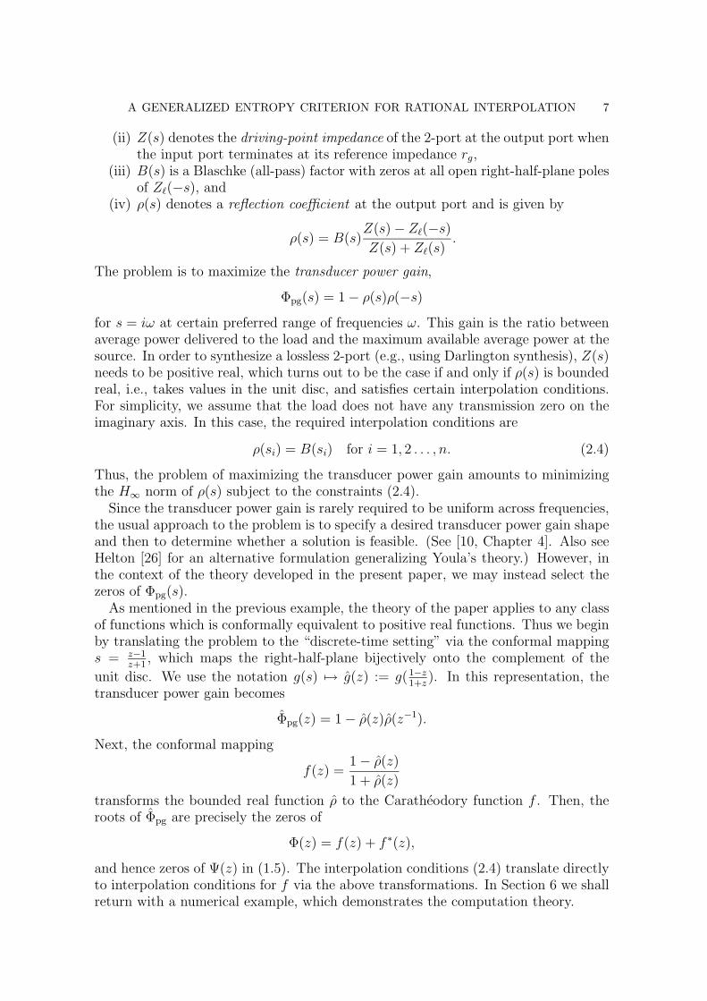
(ii) Z(s) denotes the driving-point impedance of the 2-port at the output port whenthe input port terminates at its reference impedance rg,

(iii) B(s) is a Blaschke (all-pass) factor with zeros at all open right-half-plane polesof Z`(−s), and

(iv) ρ(s) denotes a reflection coefficient at the output port and is given by

ρ(s) = B(s)Z(s)− Z`(−s)Z(s) + Z`(s)

.

The problem is to maximize the transducer power gain,

Φpg(s) = 1− ρ(s)ρ(−s)for s = iω at certain preferred range of frequencies ω. This gain is the ratio betweenaverage power delivered to the load and the maximum available average power at thesource. In order to synthesize a lossless 2-port (e.g., using Darlington synthesis), Z(s)needs to be positive real, which turns out to be the case if and only if ρ(s) is boundedreal, i.e., takes values in the unit disc, and satisfies certain interpolation conditions.For simplicity, we assume that the load does not have any transmission zero on theimaginary axis. In this case, the required interpolation conditions are

ρ(si) = B(si) for i = 1, 2 . . . , n. (2.4)

Thus, the problem of maximizing the transducer power gain amounts to minimizingthe H∞ norm of ρ(s) subject to the constraints (2.4).

Since the transducer power gain is rarely required to be uniform across frequencies,the usual approach to the problem is to specify a desired transducer power gain shapeand then to determine whether a solution is feasible. (See [10, Chapter 4]. Also seeHelton [26] for an alternative formulation generalizing Youla’s theory.) However, inthe context of the theory developed in the present paper, we may instead select thezeros of Φpg(s).

As mentioned in the previous example, the theory of the paper applies to any classof functions which is conformally equivalent to positive real functions. Thus we beginby translating the problem to the “discrete-time setting” via the conformal mappings = z−1

z+1, which maps the right-half-plane bijectively onto the complement of the

unit disc. We use the notation g(s) 7→ g(z) := g(1−z1+z

). In this representation, thetransducer power gain becomes

Φpg(z) = 1− ρ(z)ρ(z−1).

Next, the conformal mapping

f(z) =1− ρ(z)

1 + ρ(z)

transforms the bounded real function ρ to the Caratheodory function f . Then, theroots of Φpg are precisely the zeros of

Φ(z) = f(z) + f ∗(z),

and hence zeros of Ψ(z) in (1.5). The interpolation conditions (2.4) translate directlyto interpolation conditions for f via the above transformations. In Section 6 we shallreturn with a numerical example, which demonstrates the computation theory.


Example 3: Spectral estimation. Consider a scalar zero-mean, stationary Gaus-sian stochastic process y(t)Z, and denote by Φ(eiθ), θ ∈ [−π, π], its power spectraldensity. Then

Φ(z) = f(z) + f ∗(z),

where f is a Caratheodory function with the series expansion

f(z) = 12c0 + c1z

−1 + c2z−2 + . . .

about infinity, where ck = Ey(t + k)y(t) for k = 0, 1, 2, . . . . Traditionally, in orderto estimate Φ from a realization y0, y1, . . . , yN of the process, one estimates first anumber covariance samples c0, c1, . . . , cn, where n << N , via some ergodic estimatesuch as

ck =1

N + 1− n

N−n∑t=0

yt+kyk. (2.5)

Knowledge of c0, c1, . . . , cn imposes certain interpolation conditions on f at infinity.Finding all f satisfying these is the topic which originally motivated the researchprograms from which the results of the present paper emanated [17, 18, 6, 5, 4, 7, 8].A complete parameterization of all solution of degree at most n was provided in [6].

Here we shall take a radically different approach to spectral estimation that isbased on nontraditional covariance measurements. The basic idea is to determinecovariance estimates after passing the observed time series through a bank of filterwith different frequency response and then integrating these statistical measurementsin one Markovian model.

Given a number of poles, p0, p1, . . . , pn, of modulus less than one and with p0 = 0,let

Gk(z) =z

z − pkk = 0, 1, . . . , n (2.6)

form a bank of stable filters, driven by y as in Figure 5, and denote by u0, u1, . . . , un

G0(z)

G1(z)

Gn(z)

-

-

-

-

-

-

`u0

u1

un

y

Figure 8.5: Filter bank.

the corresponding output processes. For simplicity of exposition, we assume thatp0, p1, . . . , pn are distinct and real, hence, for this paper, avoiding the situation withcomplex pairs of poles. The general case will be presented in [3]. The idea is that thetransfer functions Gk are (conjugate) Cauchy kernels in the sense that

h(p−1k ) =

∫ π

−πh(eiθ)G∗(eiθ)

dθ

2π(2.7)


for any h which is analytic in Dc and square-integrable on the unit circle. To seethis, note that, if h(z) = h0 + h1z

−1 + h2z−2 + . . . , then, by orthogonality, the

integral in (2.7) equals∑∞

j=0 hjpjk = h(p−1

k ), because Gk(z) = 1 +pkz−1 +p2

kz−2 + . . . .

Therefore, assuming that the filter has come to statistical steady state, the zerothorder covariance lag of the output process uk is given by

c0(uk) := Euk(t)2 =

∫ π

−π(f(eiθ) + f∗(eiθ))|Gk(e

iθ)|2 dθ2π

= 2

∫ π

−πf(eiθ)Gk(e

iθ)G∗(eiθ)dθ

2π,

and therefore, in view of (2.7), c0(uk) = 2Gk(p−1k )f(p−1

k ). Consequently, the zerothorder covariance data for the outputs of the filter bank supply the interpolation con-straints

f(p−1k ) =

1

2(1− p2

k)c0(uk) k = 0, 1, . . . , n, (2.8)

where c0(uk), k = 0, 1, . . . , n can be determined via ergodic estimates. An advantageof this approach is interpolation of the spectrum can be chosen closer to the unit circlein precisely the frequency band where high resolution is desired. We shall return witha numerical example at the end of Section 6.

3. Preliminaries and notation

For simplicity, in this paper we only consider the case where the interpolation pointsin Z are distinct. The general case works similarly. Moreover, from now on, we assumethat the Pick (1.2) matrix is positive definite, to avoid the degenerate case where thesolution is unique. Also, for convenience, we normalize the problem so that

z0 =∞ and f(∞) is real.

This is done without loss of generality since, first, the transformation

z → 1− z0z

z − z0

sends an arbitrary z0 to infinity and is a bianalytic map from Dc into itself, and,secondly, we can subtract the same imaginary constant from all values wk withoutaltering the problem.

Denote by L2 the space of functions which are square-integrable on the unit circle.This is a Hilbert space with inner product

〈f, g〉 =1

2π

∫ π

−πf(eiθ)g∗(eiθ)dθ.

Moreover, for an f ∈ L2, let

f(eiθ) =∞∑

k=−∞fke−ikθ


be its Fourier representation. In this notation,

〈f, g〉 =∞∑

k=−∞fkgk.

Next, let H2 be the standard Hardy space of all functions which are analytic in theexterior of the unit disc, Dc, and have square-integrable limits on the boundary

limr→+1

1

2π

∫ π

−π|f(reiθ)|2dθ <∞.

As usual, H2 is identified with the subspace of L2 with vanishing negative Fouriercoefficients. More precisely, for f ∈ H2,

f(z) = f0 + f1z−1 + f2z

−2 + . . . .

The class of all Caratheodory functions in H2 will be denoted by C. Moreover, we de-note by C+ the subclass of strictly positive real functions, whose domain of analyticityincludes the unit circle and have positive real part.

Now, consider the data Z and W with the standing assumption that z0 =∞. It isa well-known consequence Beurling’s Theorem [24] that the kernel of the evaluationmap E : H2 → Cn+1 defined via

E(f) =

f(z0)f(z1)

...f(zn)

,is given by

ker(E) = BH2,

where B(z) is the Blaschke product

B(z) := z−1

n∏k=1

1− z−1k z

z − z−1k

.

Now, let H(B) be the orthogonal complement of BH2 in H2, i.e., the subspacesatisfying

H2 = BH2 ⊕H(B),

which will be referred to as the coinvariant subspace corresponding to B, since BH2

is invariant under the shift z−1. Connecting BH2 to the filter bank in Example 3in Section 2, we see that, provided zk := p−1

k for k = 0, 1, . . . , n, as suggested bythe interpolation problem, the filter-bank transfer functions (2.6) form a basis ofH(B). However, we prefer to work in a basis, g0, g1, . . . , gn, for which g0 = G0 = 1 isorthogonal to the rest of the base elements. Thus we choose

g0(z) = 1, gk(z) = Gk(z)− 1 =1

zzk − 1, k = 1, 2, . . . , n. (3.1)


For future reference, we list the four identities

〈f, g0〉 = f(∞)

〈f, gk〉 = f(zk)− f(∞), k = 1, 2, . . . , n

〈f∗, g0〉 = f(∞)

〈f∗, gk〉 = 0, k = 1, 2, . . . , n, (3.2)

which hold for all f ∈ H2. In fact, they follow readily from (2.7) and 〈f ∗, Gk〉 = f(∞)with the corresponding conjugated identities. We also remark that there is a naturalbasis for H2 obtained by extending g0, g1, . . . , gn via

gk(z) = zn+1−kB(z) for k = n+ 1, n+ 2, . . . . (3.3)

The subspace H(B) consists precisely of all rational functions of the form

p(z) =π(z)

τ(z),

where

τ(z) =n∏k=1

(z − z−1k ) (3.4)

and π(z) = π0zn+π1z

n−1+· · ·+πn is some polynomial of degree at most n. Therefore,any rational function of degree at most n can be written as

f(z) =b(z)

a(z)where a, b ∈ H(B).

Throughout the paper we shall use such representations for rational functions, andin particular the functions a(z), b(z) and σ(z), introduced in Section 1 will belong toH(B). Hence, Ψ(z), defined by (1.5) will be a symmetric pseudo-polynomial in thebasis elements of H(B) and H(B)∗. In general, the space of pseudo-polynomials inthis basis will be denoted by S, and is defined by

S = H(B) ∨H(B)∗ = spang∗n, . . . , g∗1, g0, g1, . . . , gn. (3.5)

In particular, Ψ ∈ S, and so do ab∗ and a∗b. Moreover, we define the subset

S+ = S ∈ S | S∗ = S and S(eiθ) > 0 for all θ (3.6)

of symmetric and positive functions in S. Any S ∈ S+ is a coecive spectral density.

4. A generalized entropy criterion for Nevanlinna-Pick interpolation

Given any function Ψ(z) ∈ S+, consider, for each f ∈ C+, the generalized entropygain

IΨ(f) :=1

2π

∫ π

−πlog[Φ(eiθ)]Ψ(eiθ)dθ (4.1)

where

Φ(z) := f(z) + f ∗(z). (4.2)

is the corresponding spectral density.


Entropy integrals such as (4.1) have, of course, a long history. For example, see[23, 28] for use of entropy gains in signal processing, and see [33] for use in H∞ control.The expression in formula (4.1) reduces to the standard entropy gain in the signalprocessing literature

I1(f) :=1

2π

∫ π

−πlog[f(eiθ) + f ∗(eiθ)]dθ (4.3)

when we set Ψ = 1. The unique maximizing function of I1 subject to the interpolationconstraints (1.1) can be obtained by the Nevanlinna-Pick algorithm [38] and is oftenreferred to as the central or maximum entropy solution.

Since Ψ(z) ∈ S+, there is a unique factorization

Ψ(z) = σ(z)σ∗(z) (4.4)

such that σ ∈ H(B) has no zeros in the closure of Dc, i.e., σ(z) is a minimum-phasespectral factor of Ψ(z). In particular, σ(∞) 6= 0. It turns out that there is a uniquesolution f to the Nevanlinna-Pick problem with degree constraint which maximizesthe above entropy functional. Moreover, this solution satisfies

f(z) + f ∗(z) =σ(z)σ∗(z)

a(z)a∗(z), (4.5)

where a ∈ H(B) is also minimum-phase. Hence the entropy maximization forces apreselected spectral zero structure for the interpolating function, as seen from thefollowing theorem, the proof of which will be concluded in the next section, when allnecessary lemmas have been established.

Theorem 4.1. Given a Ψ ∈ S+, there exists a unique solution to the constrainedoptimization problem

maxf∈C+

IΨ(f) (4.6)

subject to the constraints

f(zk) = wk for k = 0, 1, . . . , n. (4.7)

Moreover, this solution is of the form

f(z) =b(z)

a(z), a, b ∈ H(B), (4.8)

and hence of degree at most n, and

a(z)b∗(z) + b(z)a∗(z) = Ψ(z). (4.9)

Conversely, if f ∈ C+ satisfies conditions (4.7), (4.8) and (4.9), it is the uniquesolution of (4.6).

Theorem 4.1 provides a complete parameterization of all pairs (a, b), defining astrictly positive real solution (4.8) to the Nevanlinna-Pick problem with degree con-straint, in terms of the zeros of the minimum-phase spectral factor σ(z) of the spectraldensity Ψ ∈ S. These zeros may be chosen arbitrarily in the open unit disc.


Corollary 4.2 (Spectral Zero Assignability Theorem). To each minimum-phaseσ(z) ∈ H(B), normalized so that σ(∞) = 1, there exists a unique minimum-phasea(z) ∈ H(B) such that the unique positive real function f(z) satisfying (4.5) solvesthe interpolation problem (4.7). In other words, there is a bijective correspondencebetween pairs (a, b) solving the Nevanlinna-Pick problem with degree constraint andthe set of n points in the open unit disc, these being the zeros of σ(z).

The primal problem (4.6) is an infinite-dimensional optimization problem. However,since there are only finitely many interpolation constraints, there is a dual problemwith finitely many variables. From conditions (4.8) and (4.9), we see that

f(z) + f ∗(z) =Ψ(z)

Q(z),

where Q(z) = a(z)a∗(z) ∈ S+. In terms of the basis introduced in Section 3,

Q(z) = qng∗n(z) + . . .+ q1g

∗1(z) + q0g0(z) + q1g1(z) + . . .+ qngn(z). (4.10)

Since g0(z) ≡ 1, q0 = 〈Q, g0〉 =∫ π−π Q(eiθ)dθ. Therefore, since Q is positive on

the circle, q0 is real and positive. Hence, we may identify Q with the vector q :=(q0, q1, . . . , qn) of coefficients belonging to the set

Q+ := q ∈ R× Cn | Q(eiθ) > 0 for all θ.

Clearly, q ∈ Q+ if and only if Q ∈ S+. As we shall see shortly the q-parameters willessentially be the Lagrange multipliers for the dual problem.

Now, consider the Lagrange function

L(f, λ) = IΨ(f) + λ0(w0 − f(z0)) + 2Re

n∑k=1

λk[wk − f(zk)]

. (4.11)

Since the primal problem (4.6) amounts to maximizing a strictly concave functionover a convex region, the Lagrange function has a saddle point [32, p.458] providedthere is a stationary point in C+, and, in this case, the optimal Lagrange vector λ =(λ0, λ1, . . . , λn) ∈ Cn+1 can be determined by solving the dual problem to minimize

ρ(λ) = maxf∈C+

L(f, λ). (4.12)

Now, consider the linear map λ : Q+ → R× Cn defined by

λ0 = 2(q0 − Ren∑j=1

qj)

λk = qk for k = 1, 2, . . . , n. (4.13)

The function ρ takes finite values only for a subset of λ = (λ0, λ1, . . . , λn) ∈ R × Cnand, in particular, on the set

Λ+ := λ(Q+). (4.14)

We have the following proposition, the proof of which is deferred to Appendix A.


Proposition 4.3. For each λ ∈ Λ+, the map f 7→ L(f, λ) has a unique maximum inC+, , and it is given by

f(z) + f ∗(z) =Ψ(z)

Q(z), (4.15)

where Q is defined from (4.10) and q = λ−1(λ).

This proposition defines, for each λ ∈ Λ+, a function fλ ∈ C+, which, as is easy tocheck, can be written as

fλ(z) =1

4π

∫ π

−π

z + eiθ

z − eiθΨ(eiθ)

Qλ(eiθ)dθ

in terms of the corresponding Qλ ∈ S+. We want to show that there is a unique

minimizing λ, denoted λ, such that fλ ∈ C+ satisfies the interpolation condition

(4.7). In this case, setting f := fλ,

ρ(λ) ≥ ρ(λ) = L(f , λ), for all λ ∈ Λ+.

Now, for any f ∈ C+ which satisfies the interpolation constraints (4.7),

IΨ(f) = L(f, λ) ≤ L(f , λ).

In particular, this holds for f = f so that IΨ(f) = L(f , λ). Hence,

IΨ(f) ≤ IΨ(f) = ρ(λ) ≤ ρ(λ), (4.16)

if f satisfies the interpolation constraints. Consequently, if we can show that ρ has aminimum λ ∈ Λ+, then IΨ has a maximum in C+, and the optimal values of the twoproblems coincide.

It turns out to be more convenient to use the q’s as dual variables.

Proposition 4.4. The dual functional (4.12) is

ρ(λ(q)) = JΨ(q) + c,

where

JΨ(q) = 2w0q0 + 2Re

n∑k=1

(wk − w0)qk

− 1

2π

∫ π

−πlog[Q(eiθ)]Ψ(eiθ)dθ, (4.17)

and

c :=1

2π

∫ π

−π

(log[Ψ(eiθ)]− 1

)Ψ(eiθ)dθ.

We are now in a position to formulate the dual version of Theorem 4.1, the proof ofwhich will also be deferred to the next section. For simplicity, we remove the constantterm c, which does not affect the optimization.


Theorem 4.5. Given a Ψ ∈ S+, there exists a unique solution to the dual problem

minq∈Q+

JΨ(q). (4.18)

Moreover, to the minimizing q there corresponds an f ∈ C+ such that

Ψ(z)

Q(z)= f(z) + f ∗(z) (4.19)

where Q is given by (4.10). Moreover, this function f satisfies conditions (4.7), (4.8)and (4.9) in Theorem 4.1, namely

f(zk) = wk for k = 0, 1, . . . , n, (4.20)

f(z) =b(z)

a(z), a, b ∈ H(B), (4.21)

Ψ(z) = a(z)b∗(z) + b(z)a∗(z). (4.22)

Conversely, any f ∈ C+ which satisfies these conditions can be constructed from theunique solution of (4.18) via (4.19).

We conclude by noting that if the problem data is real or self-conjugate, and Ψ isreal, then both the function f(z) constructed above, and the function f(z), satisfythe conditions of Theorems 4.1 and 4.5 so that, by uniqueness, they must coincide.

Corollary 4.6. Assume that the the sets Z and W are self-conjugate and that wk =wj whenever zk = zj, and that Ψ is real. Then, the optimizing functions f,Q inTheorems 4.1 and 4.5 have real coefficients. In particular, there is a unique pair ofreal functions a(z) and b(z) in H(B), devoid of zeros in closure of Dc, such that

Ψ(z) = a(z)b(z−1) + a(z−1)b(z)

f(z) =b(z)

a(z)∈ C+

f(zk) = wk for k = 0, 1, ..., n.

We shall return to the special case covered in Corollary 4.6 in Section 6, and weshall refer to it as the self-conjugate case.

5. The convex optimization problem

In this section, we shall analyze the functional JΨ(q), constructed in the previoussection. We shall show that it has a unique minimum in Q+, which is instrumentalin proving Theorem 4.1 and Theorem 4.5. To this end, we first extend JΨ(q) to theclosure Q of Q+, and consider

JΨ : Q −→ R ∪ ∞.

Proposition 5.1. The functional JΨ(q) is a C∞ function on Q+ and has a continuousextension to the boundary that is finite for all q 6= 0. Moreover, JΨ is strictly convex,and Q is a closed and convex set.


This proposition, along with Propositions 5.2 and 5.4 below, are analogous to re-lated results in [7], developed for the covariance extension problem. Their proofs aresimilar, mutatis mutandis, to those developed in [7], except for Lemma 5.3 below. Thecomplete proofs are adapted to the present framework and included in the appendixfor the convenience of the reader.

In order to ensure that JΨ achieves a minimum on Q, it is important to knowwhether JΨ is proper, i.e., whether J−1

Ψ (K) is compact whenever K is compact. Inthis case, of course, a unique minimum will exist.

Proposition 5.2. For all r ∈ R, J−1Ψ (−∞, r] is compact. Thus JΨ is proper (i.e.,

J−1Ψ (K) is compact whenever K is compact) and bounded from below.

The proof of this proposition, given in the appendix, relies on the analysis of thegrowth of JΨ, which entails a comparison of linear and logarithmic growth. To thisend, the following lemma is especially important. We note that its proof is the onlypoint in our construction and argument in which we use the Pick condition in anessential way. Denote the linear part of JΨ(q) by

J(q) := 2w0q0 + 2Re

n∑k=1

(wk − w0)qk

= 2w0q0 +n∑k=1

(wk − w0)qk +n∑k=1

(wk − w0)qk. (5.1)

Lemma 5.3. For each nonzero q ∈ Q, J(q) > 0.

Proof. Since P > 0, there exists a strictly positive real interpolant. Choose an ar-bitrary such interpolant, and denote it by f . Then, recalling that z0 = ∞, (3.2)yields

2w0 = 〈f + f∗, g0〉 =1

2π

∫ π

−π[f(eiθ) + f∗(eiθ)]g∗0(eiθ)dθ

and

wk − w0 = 〈f + f∗, gk〉 =1

2π

∫ π

−π[f(eiθ) + f ∗(eiθ)]g∗k(e

iθ)dθ

for k = 1, 2, . . . , n. For any q in Q, we compute

J(q) =1

2π

∫ π

−π[f(eiθ) + f ∗(eiθ)]Q(eiθ)dθ ≥ 0,

and J(q) = 0 if and only if Q ≡ 0.

Finally, we need to exclude the possibility that the minimum occurs on the bound-ary. This is the content of the following proposition, also proved in the appendix.

Proposition 5.4. For Ψ ∈ S+, the functional JΨ never attains a minimum on theboundary ∂Q.

Hence we have established that JΨ(q) is strictly convex, has compact sublevel setsand the minimum does not occur on the boundary of Q. Consequently, it has a uniqueminimum, which occurs in the open set Q+. Clearly, this minimum point will be astationary point with vanishing gradient. As the following lemma shows, the gradient


becomes zero precisely when the interpolation conditions are satisfied, and in fact thevalue of the gradient depends only on the mismatch at the interpolation points.

Before stating the lemma, however, let us, for the convenience of the reader, reviewa few basic facts from complex function theory. In what follows, it will be convenientto use complex partial differential operators acting on smooth, but not necessarilycomplex analytic, functions. In particular, if we write the complex vector qk = xk+iykas a sum of real and imaginary parts, this defines the differential operators

∂

∂qk=

1

2

(∂

∂xk− i∂

∂yk

)and

∂

∂qk=

1

2

(∂

∂xk+ i

∂

∂yk

)which operate on smooth functions. Indeed, the second operator is the Cauchy-Riemann operator which characterizes the analytic functions F of qk via

∂F

∂qk= 0.

And, for example, while conjugation, viewed as the function defined by qk = xk− iyk,is of course not analytic, it is smooth and satisfies

∂qk∂qk

= 0 and∂qk∂qk

= 1.

Lemma 5.5. At any point q ∈ Q+ the gradient of JΨ is given by

∂JΨ

∂q0

= 2[w0 − f(z0)], (5.2)

∂JΨ

∂qk= [wk − f(zk)]− [w0 − f(z0)], for k = 1, 2, . . . , n, (5.3)

where f is the C+ function satisfying

f(z) + f ∗(z) =Ψ(z)

Q(z)(5.4)

with Q(z) ∈ S correspond to q as in (4.10).

Proof. The existence of a function f as claimed in the statement is obvious by virtue

of the fact that Ψ(z)Q(z)

is bounded and greater than zero on the unit circle. Recalling

that∂qk∂qk

= 0,

for k > 0 we have

∂JΨ

∂qk= (wk − w0)− 1

2π

∫ π

−π

g∗k(eiθ)

Q(eiθ)Ψ(eiθ)dθ

= (wk − w0)− 〈f + f∗, gk〉,which, in view of (3.2) and the fact that z0 = ∞, is the same as (5.3). For the casek = 0 we need to take the real derivative:

∂JΨ

∂q0

= 2w0 −1

2π

∫ π

−π

g0(eiθ)

Q(eiθ)Ψ(eiθ)dθ

= 2w0 − 〈f + f∗, g0〉,


which, again using (3.2), yields (5.2).

We are now prepared for the proof of our main results.

Proof of Theorem 4.5. Propositions 5.1, 5.2 and 5.4 establish the existence of a uniqueminimum in q ∈ Q+. Then Lemma 5.5 shows that the interpolation conditions aremet for the corresponding C+-function f satisfying (5.4). The construction of such afunction proceeds as follows. SinceQ ∈ S+ and is rational, it admits a rational spectral

factorization Q(z) = a(z)a∗(z), where a(z) = α(z)τ(z)

with α(z) a stable polynomial of

degree at most n. Hence, a ∈ H(B). Then, we solve the linear equation a(z)b∗(z) +b(z)a∗(z) = Ψ(z) for b. This linear equation has always a unique solution because a

has no zeros in Dc; cf. the discussion in [9]. Then f(z) = b(z)a(z)

, and all conditions of

the theorem are satisfied.Conversely, given an f ∈ C+ satisfying (4.21) and (4.22), a unique q ∈ Q+ can

be obtained from (5.4). Finally, in view of Lemma 5.5, the interpolation conditions(4.20) imply that the gradient of JΨ for the corresponding q is zero. Thus it is theunique minimizing q.

Proof of Theorem 4.1. Let us denote by q the minimizing q in Theorem 4.5. Then,since q ∈ Q+, we have λ := λ(q) ∈ Λ+ in the notation of Proposition 4.4. Let f be the

unique corresponding f ∈ C+ defined via Proposition 4.3. By Theorem 4.5, f satisfies

conditions (4.7), (4.8) and (4.9). Then, since thus f satisfies the interpolation condi-

tion, (4.16) holds, implying that f is the maximizing f of Theorem 4.1. Conversely,

if f satisfies (4.7), (4.8) and (4.9), by Theorem 4.5, the corresponding q, defined via(4.19), is the unique maximizing solution to the dual problem. Therefore, it follows

in the same way as above, that f is the unique maximizing solution to the primalproblem.

An interesting, and useful, aspect of the functionals studied using interior pointmethods is that they contain a barrier term, which is infinite on the boundary ofthe closed convex set in question. At first glance, the logarithmic integrand in JΨ(q)might seem to be a barrier-like term but, as we have seen in Section 5, by a theoremof Szego, the logarithmic integrand is in fact integrable for nonzero Q having zeros onthe boundary of the unit circle. Hence JΨ(q) does not become infinite on the entireboundary ∂Q of Q. Nonetheless, JΨ(q) has a very interesting barrier-type property asdescribed in the following proposition and proven in the Appendix.

Proposition 5.6. The dual functional JΨ(q) has an infinite gradient on the boundary∂Q.

As far as computation is concerned, this is a a useful property of the convex opti-mization problem.

6. Computational procedure

Given Ψ(z), define the class P of (strictly) positive real functions

f(z) =b(z)

a(z), a, b ∈ H(B)


having the property that

a(z)b∗(z) + b(z)a∗(z) = Ψ(z). (6.1)

We want to determine the unique function in P which also satisfies the interpolationconditions. To this end, we shall construct a sequence of functions,

f (0), f (1), f (2), · · · ∈ P

which converges to the required interpolant.As before, we may write (6.1) as

f(z) + f ∗(z) =Ψ(z)

Q(z), (6.2)

where Q ∈ S+ satisfies

a(z)a∗(z) = Q(z). (6.3)

It is easy to see that this defines a bijection

I : Q+ → P : Q 7→ f. (6.4)

To see this, note that

a(z) =α(z)

τ(z), b(z) =

β(z)

τ(z)and Ψ(z) =

d(z, z−1)

τ(z)τ ∗(z),

where α(z) and β(z) are Schur polynomials of at most degree n and d(z, z−1) is apseudo-polynomial, also of at most degree n. Then, determine α(z) via a stablepolynomial factorization

α(z)α∗(z) = τ(z)τ ∗(z)Q(z), (6.5)

and solve the linear system

α(z)β∗(z) + β(z)α∗(z) = d(z, z−1) (6.6)

for β. In fact, (6.6) is a linear (Hankel + Toeplitz) system S(α)β = d in the coefficientsof the polynomials, which is nonsingular since α(z) is a Schur polynomial; see, e.g.,[9]. Then

f(z) =β(z)

α(z).

Given an f ∈ P we can determine the corresponding gradient of JΨ(q) by means ofLemma 5.5. The following lemma gives the equations for the (n+1)× (n+1) Hessianmatrix

H(q) =

[∂2JΨ

∂qk∂q`

]nk,`=0

. (6.7)


Lemma 6.1. Let h(z) be the unique positive real function such that

h(z) + h∗(z) =Ψ(z)

Q(z)2(6.8)

and h(z0) is real. Then the Hessian (6.7) is given by

Hk`(q) =

zkz`−zkh(zk) + z`

zk−z`h(z`) + h(z0) for k 6= `; k, ` > 0

−zkh′(zk)− h(zk) + h(z0) for k = ` > 0

h(zk)− h(z0) for k > 0, ` = 0

h(z`)− h(z0) for k = 0, ` > 0

2h(z0) for k = ` = 0,

(6.9)

where h′(z) is the derivative of h(z).

Next, we turn to the computational procedure, which will be based on Newton’smethod [31, 32]. We need an f (0) ∈ P, and a corresponding Q(0) defined via (6.2),as an initial condition. We may choose Q(0) = 1. Each iteration in our procedureconsists of four steps and updates the pair f,Q to f , Q, in the following way:

Step 1. Given f , let ∇JΨ(q) be the gradient defined by (5.2) and (5.3).

Step 2. Determine the unique positive real function h satisfying (6.8), which is alinear problem of the same type as the one used to determine f from Q. In fact,exchanging α(z) for α(z)2 and d(z, z−1) for v(z, z−1) = τ(z)τ ∗(z)d(z, z−1) in (6.6) weobtain

h(z) =β(z)

α(z)2where β = S(α2)−1v.

The Hessian H(q) is then determined from h as in Lemma 6.1.

Step 3. Update Q(z) by applying Newton’s method to the function JΨ. A Newtonstep yields

qupdate = q − λH(q)−1∇JΨ(q),

where λ ∈ (0, 1] needs to chosen so that

Qupdate(eiθ) > 0 for all θ. (6.10)

This positivity condition is tested in Step 4.

Step 4. Factor Qupdate as in (6.3). This is also a test for condition (6.10). If the testfails, return to Step 3 and decrease the step size λ. If not, check whether the norm of∇JΨ(qupdate) is sufficiently small. Recall that this norm quantifies the interpolationerror, as can be seen from Lemma 5.5. If this error is small, stop; otherwise, use thelinear procedure above to determine the next iterate fupdate. Then, set f := fupdate

and return to Step 1.

The computations can be carried out quite efficiently using state space descriptions.We restrict our attention to the self-conjugate case, where both Z and W are self-conjugate and wk = wj whenever zk = zj, and Ψ(z) is real. (See Corollary 4.6.) Inparticular, we develop the steps of the algorithm so as to avoid complex arithmetic.


It is easy to see that, in this case,

τ(z) :=n∏k=1

(z − z−1k ) = zn + τ1z

n−1 + · · ·+ τn (6.11)

is a real polynomial and

B(z) = z−1 τ∗(z)

τ(z)(6.12)

is a real function, where τ∗(z) := 1 + τ1z + · · · + τnzn is the reverse polynomial. For

the rest of this section, we shall be concerned with real interpolation functions.Any real function h ∈ H(B) admits a state space representation of the form

h(z) = h0 + c(zI − A)−1h, (6.13)

where (A, h, c) are taken in the observer canonical form

A =

0 1 . . . 0...

.... . .

...0 0 . . . 1−τn −τn−1 . . . −τ1

h =

h1

h2...hn

(6.14)

c =[1, 0, . . . , 0

],

h1, h2, . . . , hn being the Markov parameters in the Taylor expansion

h(z) = h0 + h1z−1 + · · ·+ hnz

−n + . . .

about infinity. We shall use the compact notation

h =

[A hc h0

]for this representation, and keep A and c fixed when representing real functions inH(B). Since the function (6.13) is completely determined by the Markov parametersh0, h, we shall refer to them as the Markov coordinates of the function (6.13). Al-ternatively, h(z) can also be represented with respect to the standard basis in H(B)as

h(z) = h0 +n∑j=1

ηjgj(z), (6.15)

where, of course, η1, . . . , ηn are complex numbers. Finally, any h ∈ H(B) can beuniquely identified by its values at Z,

h(z0), h(z1), . . . , h(zn).

The correspondence between these three alternative representations is the content ofthe following lemma.


Lemma 6.2. Let G := [gk(zj)]j,k be the matrix (A.11), and define the Vandermonde

matrix V := [z−jk ]j,k. Then, for any h ∈ H(B),

h = V η,

where η = (η1, η2, . . . , ηn)′ is defined via (6.15), andh(z1)− h0

h(z2)− h0...

h(zn)− h0

= Gη.

Moreover, G and V are invertible.

Proof. The first correspondence follows immediately from (6.15) and the expansion

gk(z) = z−1k z−1 + z−2

k z−2 + z−3k z−3 + . . . .

The second correspondence also follows from (6.15). Finally, we already establishedinvertibility of G in the proof of Proposition 4.3, and the Vandermonde matrix V isinvertible since the points in Z are distinct.

We now reformulate the steps of the algorithm given in Section 6 in terms of thereal Markov coordinates of the relevant functions. We shall consistently work withfunctions in H(B). Therefore, as f 6∈ H(B), we form

f := ΠH(B)f,

where ΠH(B) denotes orthogonal projection onto H(B). Since f = f + Bg for asuitable g ∈ H2, it follows that

f(zk) = f(zk) for k = 0, 1, . . . , n.

Next, define w(z) to be the unique function in H(B) such that

w(zk) = wk for k = 0, 1, . . . , n. (6.16)

This function has the form w(z) = π(z)/τ(z), where τ(z) is given by (6.11), andwhere the coefficients of the polynomial π, of degree at most n, can be determined bysolving the linear (Vandermonde) system of equations defined by (6.16). The gradientof JΨ in Lemma 5.5 can then be expressed in terms of the “error function”

r(z) := w(z)− ΠH(B)f(z), (6.17)

which also belongs to H(B). In fact,

r(zk) := wk − f(zk). (6.18)

Moreover, we introduce an H(B)-representation for any Q ∈ S and any given Ψ ∈ S

by writing

Q(z) = q(z) + q∗(z), Ψ(z) = ψ(z) + ψ∗(z),


where q, ψ ∈ H(B) are positive real. Finally, we represent q and ψ by their respec-tive Markov coordinates (x, x0) and (y, y0), respectively, in the standard state-spacerepresentation described above, i.e.,

q =

[A xc x0

]and ψ =

[A yc y0

].

We begin with the state-space implementation of Step 1 in the computationalscheme described above. In this context, we have the following version of Lemma 5.5.

Proposition 6.3. Let G and V be defined as in Lemma 6.2. Given an f ∈ P, let qbe the positive real part of Q := I−1f , where I is defined as in (6.4). Moreover, letr(z) be given by (6.17), and denote by (x0, x) and (r0, r) the Markov coordinates ofq(z) and r(z) respectively. Then

∂JΨ

∂x0

= 4r0,

∂JΨ

∂x= Tr,

where T := (V ∗)−1GV −1 is a real matrix.

Proof. Since q0 = 2x0 and w0 − f(z0) = r(z0) = r0, the derivative with respect to x0

follows immediately from (5.2). Next, applying Lemma 6.2, we see that[∂xj∂qk

]nj,k=1

= V,

and that r(zk)− r0 is the k:th entry in GV −1r. Moreover, by (6.18), we have

r(zk)− r0 = [wk − f(zk)]− [w0 − f(z0)]

for k = 1, 2, . . . , n. Finally, using equation (5.3) and defining q := (q1, q2, . . . , qn)′, weobtain

∂JΨ

∂x=

([∂x

∂q

]−1)′

∂JΨ

∂q= (V ∗)−1GV −1r

establishing the rest of the proposition.

It remains to determine the projection f := ΠH(B)f . We present the constructionin two steps. Note that, since the points in Z are assumed to be distinct, z = 0 is asimple pole of B(z).

Proposition 6.4. Assume that B(z) = z−1B0(z) with B0(∞) 6= 0, and let f(z) =f0 + z−1fr(z) ∈ H2, with fr(z) ∈ H2. Then

ΠH(B)f = f0 + z−1ΠH(B0)fr(z).

Proof. First note that, for any f ∈ H2,

f := ΠH(B)f = BΠ−B∗f,


where Π− is the orthogonal projection onto the H⊥2 , the orthogonal complement of

H2 in L2. In fact, f = f + Bq for some q ∈ H2, and hence Π−B∗f = B∗f . Then,

since B∗0zf0 ∈ H⊥2 ,

f = z−1B0Π−B∗0z(f0 + z−1fr)

= f0 + z−1B0Π−B∗0fr,

from which the proposition immediately follows.

The second step given below deals with ΠH(B0)fr. Note that, while B is not inH(B), B0 is. Therefore, B0 has a state space representation with A and c given by(6.14). However, fr 6∈ H(B), so we must use other A and c matrices for fr.

Proposition 6.5. Assume that B0 ∈ H2 is a rational Blaschke product which isnonzero at infinity, and let

B0 =

[A bc d

]and fr =

[A1 b1

c1 d1

].

Then the Sylvester equation

− (A− bd−1c)X +XA1 + bd−1c1 = 0, (6.19)

has a unique solution X, and fr := ΠH(B0)fr has the state-space representation

fr =

[A b(d− − d−1d1)−Xbc dd−

], (6.20)

where

d− := −d−1c(A− bd−1c)−1(bd−1d1 +Xb1). (6.21)

Proof. We first note that B∗0(z) has the state-space description

B∗0 =

[A0 b0

c0 d0

]with A0 = A− bd−1c, b0 = bd−1, c0 = −d−1c and d0 = d−1 and with A0 having all itseigenvalues outside the unit disc. Consider the Lyapunov equation

X − A−10 XA1 − A−1

0 b0c = 0,

which has a unique solution since both A1 and A−10 have eigenvalues inside the unit

disc [16]. But then so does

−A0X +XA1 + b0c1 = 0,

which is the same as (6.19). Using standard manipulations (see, e.g., [15, p.IX]), itfollows that B∗0fr has the state space form

B∗0fr =

A0 0 b0d1 +Xb1

0 A1 b1

c0 d0c1 − c0X d0d1

.


Next, consider f(z) := Π−B∗0fr, which has the representation

f =

[A0 b0d1 +Xb1

c0 d−

], d− := c0A

−10 (b0d1 +Xb1),

where the nontrivial d-term is due to the fact that f(z) being in H⊥2 must vanish at

the origin. The final step needed to obtain a canonical realization for fr := B0f , isstandard and involves cancellation of the unobservable modes at the poles of f . Notethat these poles coincide with the zeros of B0.

Consequently, the state-space version of Step 1 amounts to solving the Sylvesterequation (6.19) to obtain fr. Then the gradient is determined from

r(z) = w(z)− f0 − z−1fr(z),

as described in Proposition 6.3. Step 2 is developed along the same lines as in Step 1by instead representing relevant functions in H(B2). Then a Newton step is taken asdescribed in Step 3. Alternatively, a gradient method is used, in which case Step 2 canbe deleted. Finally, Step 4, i.e., determining f from q, amounts to solving a matrixRiccati equation and a Lyapunov equation, as seen from the following proposition.

Proposition 6.6. Suppose that q, ψ ∈ H(B) are strictly positive real with Markov pa-rameters (x, x0) and (y, y0), respectively. Let P be the unique solution to the algebraicRiccati equation

P = APA′ + (x− APc′)(2x0 − cPc′)−1(x− APc′)′, (6.22)

d1 := (2x0 − cPc′)1/2,

b1 := (x− APc′)d−11 ,

having the property that

Γ := A− b1d−11 c′ (6.23)

is stable, and let X be the unique solution of the Lyapunov equation

X = ΓXΓ′ + yy−10 y′ − (y − b1d

−11 y0)y−1

0 (y − b1d−11 y0)′, (6.24)

d2 := 12(y0 − cXc′)d−1

1 ,

b2 := [(y − Axc′)− b1d2]d−11 .

Then f = I(q + q∗), defined as in (6.4), has the state-space representation

f =

[Γ b1d

−11 d2 − b2

−d−11 c d−1

1 d2

].

Proof. Observe that determining a(z) from q+ q∗ = aa∗ is a standard spectral factor-ization problem [1, 14] with the unique minimum-phase solution given by

a =

[A b1

c d1

].

Then b(z) is determined from the linear equation

Ψ = ψ + ψ∗ = ab∗ + ba∗


which, in the state-space formulation, becomes (6.24). Since Γ is stable, it has aunique solution X. Finally, the state space description of f = a−1b is obtained bydirect computation, using the formalism in, e.g., [15, p.IX].

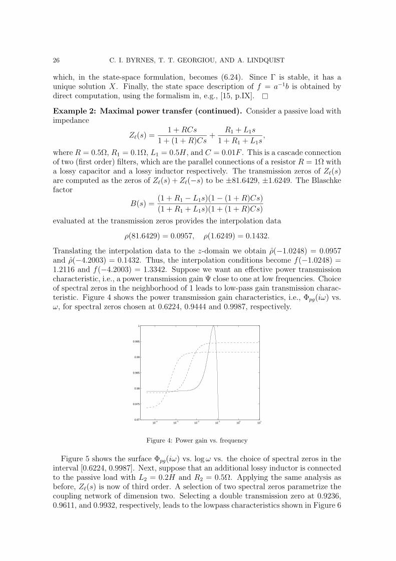
Example 2: Maximal power transfer (continued). Consider a passive load withimpedance

Z`(s) =1 +RCs

1 + (1 +R)Cs+

R1 + L1s

1 +R1 + L1s,

where R = 0.5Ω, R1 = 0.1Ω, L1 = 0.5H, and C = 0.01F . This is a cascade connectionof two (first order) filters, which are the parallel connections of a resistor R = 1Ω witha lossy capacitor and a lossy inductor respectively. The transmission zeros of Z`(s)are computed as the zeros of Z`(s) +Z`(−s) to be ±81.6429, ±1.6249. The Blaschkefactor

B(s) =(1 +R1 − L1s)(1− (1 +R)Cs)

(1 +R1 + L1s)(1 + (1 +R)Cs)

evaluated at the transmission zeros provides the interpolation data

ρ(81.6429) = 0.0957, ρ(1.6249) = 0.1432.

Translating the interpolation data to the z-domain we obtain ρ(−1.0248) = 0.0957and ρ(−4.2003) = 0.1432. Thus, the interpolation conditions become f(−1.0248) =1.2116 and f(−4.2003) = 1.3342. Suppose we want an effective power transmissioncharacteristic, i.e., a power transmission gain Ψ close to one at low frequencies. Choiceof spectral zeros in the neighborhood of 1 leads to low-pass gain transmission charac-teristic. Figure 4 shows the power transmission gain characteristics, i.e., Φpg(iω) vs.ω, for spectral zeros chosen at 0.6224, 0.9444 and 0.9987, respectively.

10−4

10−3

10−2

10−1

100

101

0.97

0.975

0.98

0.985

0.99

0.995

1

Figure 4: Power gain vs. frequency

Figure 5 shows the surface Φpg(iω) vs. logω vs. the choice of spectral zeros in theinterval [0.6224, 0.9987]. Next, suppose that an additional lossy inductor is connectedto the passive load with L2 = 0.2H and R2 = 0.5Ω. Applying the same analysis asbefore, Z`(s) is now of third order. A selection of two spectral zeros parametrize thecoupling network of dimension two. Selecting a double transmission zero at 0.9236,0.9611, and 0.9932, respectively, leads to the lowpass characteristics shown in Figure 6


(dashed curves correspond to the first two choices while a continuous curve indicatesthe last one with a slighly wider bandwidth).

−4−3.5−3−2.5−2−1.5−1−0.50

0.65

0.7

0.75

0.8

0.85

0.9

0.95

0.96

0.97

0.98

0.99

1

Figure 5: Power gain vs. frequency vs. zero location

10−4

10−3

10−2

0.97

0.975

0.98

0.985

0.99

0.995

1

Figure 6: Power gain vs. frequency

At the present time, in high order cases, there is no systematic way to select trans-mission zeros that could produce the exact desired shape of the power transmissiongain.

Example 3: Spectral estimation (continued). Consider a bank of three filtersas in Figure 5, with (z0, z1, z2) = (∞, 2, 1.5). Assume that the resulting values forc0(uk), which specify f(z) at these points, give interpolating values (w0, w1, w2) =(1, 1.2, 1.1). We would like to construct a model with an all-pole spectral density.Traditional techniques based on the Levinson algorithm are not applicable since theinterpolation data are not in the form of a partial covariance sequence. Furthermore,the “central solution” corresponding to Ψ(s) = 1 leads to filters with spectral zerosat z−1

1 , z−12 , . . . , z−1

n , whereas we are interested in an AR model, i.e., one with all zerosat the origin. Selecting Ψ(z) = 1

τ(z)τ(z−1), where τ(z) = (z − 1/2)(z − 2/3), and using


our algorithm, we obtain

f(z) =(z − 0.6829)(z + 0.8677)

(z − 0.3612)2 + 0.67972.

Note that the zeros of f(z) are at 0.6829 and at −0.8677, while there are no spectralzeros in the unit disc. The corresponding all-pole spectral density f(z) + f(z−1) isdepicted in Figure 6.

0 0.5 1 1.5 2 2.5 3 3.50

1

2

3

4

5

6

7

8

Figure 7: |Φ(eiθ)| as a function of θ

A natural question regarding this example is why one would want to use Nevanlinna-Pick data for determinig an autoregressive model, when such a model can be obtainedfrom traditional covariance data simply using the Levinson algorithm. The advantagein using Nevanlinna-Pick data is discussed in [3] where it is shown that a suitableselection of filterbank poles enhances resolution beyond what can be obtained withtraditional covariance estimates. Intuitively, interpolation in the vicinity of an arcof the unit circle specifies more accurately the shape of f , and hence the spectraldensity, in that part of the spectrum.

7. Conclusions

In this paper, we have given a method for finding all solutions to the scalar, rationalNevanlinna-Pick interpolation problem, having degree less than or equal to n, interms of the minima of a parameterized family of convex optimization problems.While the problem has been posed for positive real interpolants, as would arise forthe control of discrete-time systems, standard linear fractional transformations canadapt this generalized entropy criterion approach to positive real, or bounded-real,transfer functions for both continuous and discrete-time linear systems.

Appendix A. Proofs of deferred propositions and lemmas

Proof of Proposition 4.3. We note that C+ ⊂ H2, and we consider the representation

f(z) =∞∑j=0

fjgj(z). (A.1)


Based on our standing assumptions on f(z), and our choice of the basis (3.1), (3.3),we have f0 = f(∞) is real, while fk, k = 1, 2, . . . , are allowed to be complex. Thus,we identify f(z) with the vector of coefficients f := (f0, f1, . . . ), and define the set

F = f ∈ `2 | f0 ∈ R, f1, f2, · · · ∈ C,∞∑j=0

fjgj(z) ∈ C+. (A.2)

Since B(zk) = 0 for k = 0, 1, 2, . . . , n, we have gj(zk) = 0 for j > n, and consequently

f(zk) =n∑j=0

fjgj(zk). (A.3)

Suppose that λ ∈ Λ+. The function f → L(f, λ) is strictly concave, so, if it has astationary point where the gradient is zero, it has a unique maximum there. Thus,we set ∂L

∂fk= 0 for all k. Since f0 is real and g0 = 1, we then have

∂L

∂f0

= 21

2π

∫ π

−πΦ−1(eiθ)Ψ(eiθ)dθ − λ0 − 2Re

n∑k=1

λk

= 0. (A.4)

Furthermore, referring back to the discussion on function theory before Lemma 5.5,

we recall that ∂fk∂fk

= 0 and ∂fk∂fk

= 1. Therefore, in view of (A.3), we obtain

∂L

∂fk=

1

2π

∫ π

−πgk(e

iθ)Φ−1(eiθ)Ψ(eiθ)dθ −n∑j=1

λjgk(zj) = 0 (A.5)

for k = 1, 2, . . . , n, and

∂L

∂fk=

1

2π

∫ π

−πgk(e

iθ)Φ−1(eiθ)Ψ(eiθ)dθ = 0 (A.6)

for k = n+ 1, n+ 2, . . . , where we have used the orthogonality properties discussed inSection 3. Now, let Q(z) := Φ−1(z)Ψ(z), and note that Q∗(z) = Q(z). From (A.6),

〈Q, gk〉 = 0 = 〈Q, g∗k〉 for k = n+ 1, n+ 2, . . . .

Hence Q ∈ S, having a representation (4.10) with q0 ∈ R and q1, . . . , qn ∈ C. By con-struction, (4.15) holds, and therefore it remains to show that Q ∈ S+ or, equivalently,that q ∈ Q+, to establish that f ∈ C+, proving the proposition.

From (A.4), we immediately see that

λ0 = 2q0 − 2Re

n∑j=1

λj

. (A.7)

Next, taking the conjugate of (A.5) we obtain

〈Q, gk〉 =n∑j=1

λj gk(zj) (A.8)


for k = 1, 2, . . . , n. On the other hand,

〈Q, gk〉 =n∑j=1

qjgj(zk). (A.9)

Since gk(zj) = gj(zk), by (A.8) and (A.9),g1(z1) g2(z1) · · · gn(z1)g1(z2) g2(z2) · · · gn(z2)

......

. . ....

g1(zn) g2(zn) · · · gn(zn)

λ1 − q1

λ2 − q2...

λn − qn

= 0. (A.10)

Now, it is easy to see that the coefficient matrix

G =

[z−1k z−1

`

1− z−1k z−1

`

]nk,`=1

, (A.11)

of the linear system (A.10) is nonsingular, and therefore

λk = qk for k = 1, 2, . . . , n. (A.12)

In fact, G = 12Z∗PZ, where Z is the diagonal matrix diag(z−1

1 , . . . , z−1n ) and P is the

Pick matrix for Z = z1, . . . , zn and W = 1, . . . , 1, which is positive definite, byassumption.

Equations (A.7) and (A.12) establish that λ = λ(q). Therefore, since λ ∈ Λ+, wehave q ∈ Q+, as required.

Proof of Proposition 4.4. Applying the linear map (4.13), the dual functional (4.12)can be expressed in terms of q := (q0, q1, . . . , qn). In fact,

ρ(λ(q)) = − 1

2π

∫ π

−πlog[Q(eiθ)]Ψ(eiθ)dθ +

1

2π

∫ π

−πlog[Ψ(eiθ)]Ψ(eiθ)dθ

+

(2q0 − 2Re

n∑j=1

qj

)(w0 − f0) + 2Re

n∑j=1

qj[wj − f(zj)]

.(A.13)

In this expression the sum of the two last terms turns out to be linear in q. To seethis and eliminate the dependence of f ’s on the q’s, consider the following:

1

2π

∫ π

−πΨ(eiθ)dθ =

1

2π

∫ π

−πQ(eiθ)Φ(eiθ)dθ

= q0〈f + f∗, g0〉+ 2Re

n∑j=1

qj〈f + f∗, gj〉

= 2q0f0 + 2Re

n∑j=1

qj(f(zj)− f0)

.


Using this last expression, the dual function becomes

ρ(λ(q)) = − 1

2π

∫ π

−πlog[Q(eiθ)]Ψ(eiθ)dθ +

1

2π

∫ π

−πlog[Ψ(eiθ)]Ψ(eiθ)dθ

− 1

2π

∫ π

−πΨ(eiθ)dθ + 2q0w0 + 2Re

n∑j=1

qj(wj − w0)

. (A.14)

In this expression, define c to be the sum of the second and third terms. Then, theproposition follows.

Proof of Proposition 5.1. We want to prove that JΨ(q) is finite when q 6= 0. Then therest follows by inspection. Clearly, JΨ(q) cannot take the value −∞; hence it remainsto prove that JΨ(q) <∞. Since q 6= 0,

µ := maxθQ(eiθ) > 0.

Then, setting P (z) := µ−1Q(z),

logP (eiθ) ≤ 0 (A.15)

and

JΨ(q) = J(q)− 1

2πlog µ

∫ π

−πΨ(eiθ)dθ − 1

2π

∫ π

−πlog[P (eiθ)]Ψ(eiθ)dθ,

and hence the question of whether JΨ(q) <∞ is reduced to determining whether

−∫ π

−πlog[P (eiθ)]Ψ(eiθ)dθ <∞.

But, since Ψ(eiθ) ≤M for some bound M , this follows from∫ π

−πlogP (eiθ)dθ > −∞, (A.16)

which is the well-known Szego condition: (A.16) is a necessary and sufficient conditionfor P (eiθ) to have a stable spectral factor [22]. But, since the rational function P (z)belongs to S+, there is a function π(z) ∈ H(B) such that π(z)π∗(z) = P (z). Butthen π(z) is a stable spectral factor of P (z), and hence (A.16) holds.

Proof of Proposition 5.2. Suppose q(k) is a sequence in Mr := J−1Ψ (−∞, r]. It suffices

to show that q(k) has a convergent subsequence. The sequence q(k) defines a sequenceof unordered n-tuples of zeros lying in the the unit disc, and a sequence of scalarmultipliers. We wish to prove that both of these sequences cluster. To this end, eachQ(k) may be factored as

Q(k)(z) = λkak(z)a∗k(z) = λkQ

(k)(z),

where λk is positive and ak(z) is a function in H(B) which is normalized so thatak(∞) = 1.

We shall first show that the sequence of zeros clusters. The corresponding sequenceof the (unordered) set of n zeros of each ak(z) has a convergent subsequence, sinceall (unordered) sets of zeros lie in the closed unit disc. Denote by a(z) the functionin H(B) which vanishes at this limit set of zeros and which is normalized so thata(∞) = 1. By reordering the sequence if necessary, we may assume the sequence


ak(z) tends to a(z). Therefore the sequence q(k) has a convergent subsequence if andonly if the sequence λk does.

We now show that the sequence of multipliers, λk, clusters. It suffices to prove thatthe sequence λk is bounded from above and from below away from zero. This willfollow by analyzing the linear and the logarithmic growth in

JΨ(q(k)) = J(q(k))− 1

2πlog λk

∫ π

−πΨ(eiθ)dθ − 1

2π

∫ π

−πlog[Q(k)(eiθ)]Ψ(eiθ)dθ

with respect to the sequence λk. Here J(q) is the linear term (5.1) of JΨ(q). We firstnote that the sequence J(q(k)), where q(k) is the vector corresponding to the pseudo-polynomial Q(k), is bounded from above because the normalized functions ak(z) lie ina bounded set. Similarly, by the proof of Lemma 5.3, the sequence J(q(k)) is boundedfrom below, away from zero. In particular, the coefficient of λk in the first term forthis expression for JΨ(q(k)) is bounded away from 0 and away from ∞. We also notethat the coefficient of log λk in this expression for JΨ(q(k)) is independent of k. Next,the term

1

2π

∫ π

−πlog[Q(k)(eiθ)]Ψ(eiθ)dθ (A.17)

in this expression for JΨ(q(k)) is independent of λk, and we claim that it remainsbounded as a function of k. Indeed, are both bounded from above and from belowrespectively away from zero and −∞. The upper bounds come from the fact thatRe〈w+1, q(k)〉 are Schur polynomials and hence have their coefficients in the boundedSchur region. In fact,

Q(k)(eiθ)→ |a(eiθ)|2 = Q(z)

where a(z) has all its zeros in the closed unit disc. In particular, if q in Q correspondsto q, then the third term in the expression for JΨ(q(k)) converges to JΨ(q), which isfinite since a is not identically zero.

Finally, observe that if a subsequence of λk were to tend to zero, then JΨ(q(k))would exceed r. Likewise, if a subsequence of λk were to tend to infinity, JΨ wouldexceed r, since linear growth dominates logarithmic growth.

Proof of Proposition 5.4. Denoting by DpJΨ(q) the directional derivative of JΨ at qin the direction p, it is easy to see that

DpJΨ(q) := limε→0

JΨ(q + εp)− JΨ(q)

ε

= J(p)− 1

2π

∫ π

−π

P (eiθ)

Q(eiθ)Ψ(eiθ)dθ, (A.18)

where P (z) is the pseudo-polynomial

P (z) = png∗n(z) + . . .+ p1g

∗1(z) + p0g0(z) + p1g1(z) + . . .+ pngn(z)

corresponding to the vector p ∈ Cn+1. In fact,

log(Q+ εP )− logQ

ε=P

Qlog

[(1 + ε

P

Q)

1εQP

]→ P

Q

as ε→ +0, and hence (A.18) follows by dominated convergence.


Now, let q ∈ Q+ and q ∈ ∂Q be arbitrary. Then the corresponding pseudo-polynomials Q and Q have the properties

Q(eiθ) > 0 for all θ ∈ [−π, π]

and

Q(eiθ) ≥ 0 for all θ and Q(eiθ0) = 0 for some θ0.

Since qλ := q + λ(q − q) ∈ Q+ for λ ∈ (0, 1], we also have for λ ∈ (0, 1] that

Qλ(eiθ) := Q(eiθ) + λ[Q(eiθ)− Q(eiθ)] > 0, for all θ ∈ [−π, π],

and we may form the directional derivative

Dq−qJΨ(qλ) = J(q − q) +1

2π

∫ π

−πhλ(θ)dθ, (A.19)

where

hλ(θ) = −Q(eiθ)− Q(eiθ)

Qλ(eiθ)Ψ(eiθ).

Now,

d

dλhλ(θ) =

[Q(eiθ)− Q(eiθ)]2

Qλ(eiθ)2Ψ(eiθ) ≥ 0,

and hence hλ(θ) is a monotonely nondecreasing function of λ for all θ ∈ [−π, π].Consequently hλ tends pointwise to h0 as λ→ 0. Therefore,

1

2π

∫ π

−πhλ(θ)dθ → +∞ as λ→ 0. (A.20)

In fact, if

1

2π

∫ π

−πhλ(θ)dθ → α <∞ as λ→ 0, (A.21)

then hλ is a Cauchy sequence in L1(−π, π) and hence has a limit in L1(−π, π) whichmust equal h0 a.e. But h0, having poles in [−π, π], is not summable and hence, asclaimed, (A.21) cannot hold.

Consequently, by virtue of (A.19),

Dq−qJΨ(qλ)→ +∞ as λ→ 0 (A.22)

for all q ∈ Q+ and q ∈ ∂Q, and hence, in view of Lemma 26.2 in [34], JΨ is essentiallysmooth. Then it follows from Theorem 26.3 in [34] that the subdifferential of JΨ isempty on the boundary of Q, and therefore JΨ cannot have a minimum there.

Proof of Proposition 5.6. The proof follows directly from (A.22)

Proof of Lemma 6.1. For k, ` = 0, 1, . . . , n we have

∂2JΨ

∂qk∂q`=

1

2π

∫ π

−πg∗k(e

iθ)g∗` (eiθ)

Ψ(eiθ)

Q(eiθ)2dθ (A.23)

= 〈(h+ h∗)g∗` , gk〉. (A.24)


For ` = 0 this becomes 〈h, gk〉+〈h∗, gk〉, which, in view of (3.2), becomes h(zk)−h(z0)if k > 0 and 2h(z0) if k = 0. For k, ` > 0, we have 〈h∗g∗` , gk〉 = 0 and therefore

∂2JΨ

∂qk∂q`=

1

2π

∫ π

−πg∗k(e

iθ)g∗` (eiθ)h(eiθ)dθ.

There are two cases. First, suppose k 6= `. Then a simple calculation yields

g∗k(z)g∗` (z) =

zkz` − zk

g∗k(z) +z`

zk − z`g∗` (z),

and hence∂2JΨ

∂qk∂q`=

zkz` − zk

〈h, gk〉+z`

zk − z`〈h, g`〉,

which, by (3.2), yields those elements of the Hessian for which k 6= ` and k, ` > 0.Secondly, suppose that k = `. Since

g∗k(z) =z

zk − z= −1 +

zkzk − z

,

we obtain

∂2JΨ

∂2qk= −〈h, gk〉+

1

2π

∫ π

−π

zkeiθ

(zk − eiθ)2h(eiθ)dθ. (A.25)

To compute the second term in (A.25), differentiate h(z), which is given, as above,by the Cauchy formula

h(z)− h(z0) =1

2π

∫ π

−π

eiθ

z − eiθh(eiθ)dθ.

Then

h′(z) = − 1

2π

∫ π

−π

eiθ

(z − eiθ)2h(eiθ)dθ,

which, together with (A.25) and (3.2), proves the remaining part of the lemma.

References

1. B. D. O. Anderson, The inverse problem of stationary convariance generation, J. StatisticalPhysics 1 (1969), 133–147.

2. C. I. Byrnes, P. Enqvist, and A. Lindquist, Cepstral coefficients, covariance lags and pole-zeromodels for finite data strings, submitted for publication.

3. C. I. Byrnes, T. T. Georgiou, and A. Lindquist, A new approach to Spectral Estimation: Atunable high-resolution spectral estimator, IEEE Trans. Signal Processing, to be published.

4. C. I. Byrnes and A. Lindquist, On duality between filtering and control, in Systems and Controlin the Twenty-First Century, C. I. Byrnes, B. N. Datta, D. S. Gilliam and C. F. Martin, editors,Birhauser, 1997, pp. 101–136.

5. C. I. Byrnes and A. Lindquist, On the partial stochastic realization problem, IEEE Trans. Auto-matic Control AC-42 (1997), 1049–1069.

6. C. I. Byrnes, A. Lindquist, S. V. Gusev, and A. S. Matveev, A complete parametrization of allpositive rational extensions of a covariance sequence, IEEE Trans. Automatic Control AC-40(1995), 1841–1857.

7. C. I. Byrnes, S. V. Gusev and A. Lindquist, A convex optimization approach to the rationalcovariance extension problem, SIAM J. Control and Optimization, SIAM J. Control and Opti-mization, 37 (1999), 211–229.


8. C. I. Byrnes, H. J. Landau and A. Lindquist, On the well-posedness of the rational covarianceextension problem, in Current and Future Directions in Applied Mathematics, M. Alber, andB. Hu, J. Rosenthal, editors, Birhauser Boston, 1997, pp. 83–108.

9. C. I. Byrnes, A. Lindquist and Y. Zhou, On the nonlinear dynamics of fast filtering algorithms,SIAM J. Control and Optimization, 32(1994), 744–789.

10. W-K. Chen, Theory and Design of Broadband Matching Networks, Pergamon Press, 1976.11. Ph. Delsarte, Y. Genin and Y. Kamp, On the role of the Nevanlinna-Pick problem in circuits

and system theory, Circuit Theory and Applications 9 (1981), 177–187.12. Ph. Delsarte, Y. Genin, Y. Kamp and P. van Dooren, Speech modelling and the trigonometric

moment problem, Philips J. Res. 37 (1982), 277–292.13. J. C. Doyle, B. A. Frances and A. R. Tannenbaum, Feedback Control Theory, Macmillan Publ.

Co., New York, 1992.14. P. Faurre, M. Clerget, and F. Germain, Operateurs Rationnels Positifs, Dunod, 1979.15. B. A. Francis, A Course in H∞ Control Theory, Springer-Verlag, 1987.16. F. R. Gantmacher, The Theory of Matrices, Chelsea, New York, 1959.17. T. T. Georgiou, Partial realization of covariance sequences, CMST, Univ. Florida, Gainesville,

1983.18. T. T. Georgiou, Realization of power spectra from partial covariance sequences, IEEE Transac-

tions Acoustics, Speech and Signal Processing ASSP-35 (1987), 438–449.19. T. T. Georgiou, A topological approach to Nevanlinna-Pick interpolation, SIAM J. Math. Anal-

ysis 18 (1987), 1248–1260.20. T. T. Georgiou, The interpolation problem with a degree constraint, 44(3): 631-635, 1999.21. B. K. Ghosh, Transcendental and interpolation methods in simultaneous stabilization and simul-

taneous partial pole placement problems, SIAM J. Control and Optim. 24 (1986), 1091–1109.22. U. Grenander and M. Rosenblatt, Statistical Analysis of Stationary Time Series, Almqvist &

Wiksell, Stockholm, 1956.23. S. Haykin, Nonlinear Methods of Spectral Analysis, Springer-Verlag, 1983.24. H. Helson, Lectures on Invariant Subspaces, Academic Press, New York, 1964.25. J. W. Helton, Non-Euclidean analysis and electronics, Bull. Amer. Math. Soc. 7 (1982), 1–64.26. J. W. Helton, The distance from a function to H∞ in the Poincare metric: Electrical power

transfer, J. of Functional Analysis, 38 (1980), 273-314.27. R. E. Kalman, Realization of covariance sequences, Proc. Toeplitz Memorial Conference (1981),

Tel Aviv, Israel, 1981.28. S. A. Kassam and H. V. Poor, Robust techniques for signal processing, Proceedings IEEE 73

(1985), 433–481.29. P. P. Khargonekar and A. Tannenbaum, Non-Euclidean metrics and robust stabilization of sys-

tems with parameter uncertainty, IEEE Trans. Automatic Control AC–30 (1985), 1005–1013.30. H. Kimura, Robust stabilizability for a class of transfer functions IEEE Trans. Automatic Control

AC–29 (1984), 788–793.31. D. G. Luenberger, Linear and Nonlinear Programming (Second Edition), Addison-Wesley Pub-

lishing Company, Reading, Mass., 1984.32. M. Minoux, Jr., Mathematical Programming: Theory and Algorithms, Wiley, 1986.33. D. Mustafa and K. Glover, Minimum Entropy H∞ Control, Springer Verlag, Berlin, 1990.34. R. T. Rockafellar, Convex Analysis, Princeton University Press, 1970.35. D. Sarason, generalized interpolation in H∞, Trans. Amer. Math. Soc. 127 (1967), 179–203.36. A. Tannenbaum, Feedback stabilization of linear dynamical plants with uncertainty in the gain

factor, Int. J. Control 32 (1980), 1–16.37. A. Tannenbaum, Modified Nevanlinna-Pick interpolation of linear plants with uncertainty in the

gain factor, Int. J. Control 36 (1982), 331–336.38. J. L. Walsh, Interpolation and Approximation by Rational Functions in the Complex Domain,

Amer. Math.Soc. Colloquium Publications, 20, Providence, R. I., 1956.39. D. C. Youla and M. Saito, Interpolation with positive-real functions, J. Franklin Institute 284

(1967), 77–108.40. G. Zames and B. A. Francis, Feedback, minimax sensitvity, and optimal robust robustness, IEEE


Transactions on Automatic Control AC–28 (1983), 585–601.41. K. Zhou, Essentials of Robust Control, Prentice-Hall, 1998.

a generalized entropy criterion for nevanlinna-pick...

Documents