A General System for Heuristic Solution of ConvexProblems over Nonconvex Sets

Steven Diamond Reza Takapoui Stephen Boyd

January 28, 2016

Abstract

We describe general heuristics to approximately solve a wide variety of problemswith convex objective and decision variables from a nonconvex set. The heuristics,which employ convex relaxations, convex restrictions, local neighbor search methods,and the alternating direction method of multipliers (ADMM), require the solution ofa modest number of convex problems, and are meant to apply to general problems,without much tuning. We describe an implementation of these methods in a pack-age called NCVX, as an extension of CVXPY, a Python package for formulating andsolving convex optimization problems. We study several examples of well known non-convex problems, and show that our general purpose heuristics are effective in findingapproximate solutions to a wide variety of problems.

1 Introduction

1.1 The problem

We consider the optimization problem

minimize f0(x, z)subject to fi(x, z) ≤ 0, i = 1, . . . ,m

Ax+Bz = cz ∈ C,

(1)

where x ∈ Rn and z ∈ Rq are the decision variables, A ∈ Rp×n, B ∈ Rp×q, c ∈ Rp

are problem data, and C ⊆ Rq is compact. We assume that the objective and inequalityconstraint functions f0, . . . , fm : Rn × Rq → R are jointly convex in x and z. When theset C is convex, (1) is a convex optimization problem, but we are interested here in thecase where C is not convex. Roughly speaking, the problem (1) is a convex optimizationproblem, with some additional nonconvex constraints, z ∈ C. We can think of x as thecollection of decision variables that appear only in convex constraints, and z as the decisionvariables that are directly constrained to lie in the (generally) nonconvex set C. The set C

1

arX

iv:1

601.

0727

7v1

[m

ath.

OC

] 2

7 Ja

n 20

16

is often a Cartesian product, C = C1 × · · · × Ck, where Ci ⊂ Rqi are sets that are simple todescribe, e.g., Ci = {0, 1}. We denote the optimal value of the problem (1) as p?, with theusual conventions that p? = +∞ if the problem is infeasible, and p? = −∞ if the problem isunbounded below.

1.2 Special cases

Mixed-integer convex optimization. When C = {0, 1}q, the problem (1) is a generalmixed integer convex program, i.e., a convex optimization problem in which some variablesare constrained to be Boolean. (Mixed Boolean convex program would be a more accuratename for such a problem, but ‘mixed integer’ is commonly used.) It follows that the prob-lem (1) is hard; it includes as a special case, for example, the general Boolean satisfactionproblem.

Cardinality constrained convex optimization. As another broad special case of (1),consider the case C = {z ∈ Rq | card(z) ≤ k, ‖z‖∞ ≤M}, where card(z) is the number ofnonzero elements of z, and k and M are given. We call this the general cardinality-constrainedconvex problem. It arises in many interesting applications, such as regressor selection.

Other special cases. As we will see in §6, many (hard) problems can be formulated inthe form (1). More examples include regressor selection, 3-SAT, circle packing, the travelingsalesman problem, factor analysis modeling, job selection, the maximum coverage problem,inexact graph isomorphism, and many more.

1.3 Convex relaxation

Convex relaxation of a set. A compact set C always has a tractable convex relaxation.By this we mean a (modest-sized) set of convex inequality and linear equality constraintsthat hold for every z ∈ C:

z ∈ C =⇒ hi(z) ≤ 0, i = 1, . . . , s, Fz = g.

We will assume that these relaxation constraints are included in the convex constraintsof (1). Adding these relaxation constraints to the original problem yields an equivalentproblem (since the added constraints are redundant), but can improve the convergence ofany method, global or heuristic. By tractable, we mean that the number of added constraintsis modest, and in particular, polynomial in q.

For example, when C = {0, 1}q, we have the inequalities 0 ≤ zi ≤ 1, i = 1, . . . , q. (Theseinequalities define the convex hull of C, i.e., all other convex inequalities that hold for allz ∈ C are implied by them.) When

C = {z ∈ Rq | card(z) ≤ k, ‖z‖∞ ≤M},

2

we have the convex inequalities

‖z‖1 ≤ kM, ‖z‖∞ ≤M.

(These inequalities define the convex hull of C.) For general compact C the inequality ‖z‖∞ ≤M will always be a convex relaxation for some M .

Relaxed problem. If we remove the nonconvex constraint z ∈ C, we get a convex relax-ation of the original problem:

minimize f0(x, z)subject to fi(x, z) ≤ 0, i = 1, . . . ,m

Ax+Bz = c.(2)

(Recall that convex equalities and inequalities known to hold for z ∈ C have been incorpo-rated in the convex constraints.) The relaxed problem is convex; its optimal value is a lowerbound on the optimal value p? of (1). A solution (x∗, z∗) to problem (2) need not satisfyz∗ ∈ C, but if it does, the pair (x∗, z∗) is optimal for (1).

1.4 Projections and approximate projections

Our methods will make use of tractable projection, or tractable approximate projection, ontothe set C. The usual Euclidean projection onto C will be denoted Π. (It need not be uniquewhen C is not convex.) By approximate projection, we mean any function Π : Rq → C thatsatisfies Π(z) = z for z ∈ C. For example, when C = {0, 1}q, exact projection is given byrounding the entries to {0, 1}.

As a less trivial example, consider the cardinality-constrained problem. The projectionof z onto C is given by

(Π (z))i =

M zi > M, i ∈ I−M zi < −M, i ∈ Izi |zi| ≤M, i ∈ I0 i 6∈ I,

where I ⊆ {1, . . . , q} is a set of indices of k largest values of |zi|. We will describe manyprojections, and some approximate projections, in §4.

1.5 Residual and merit functions

For any (x, z) with z ∈ C, we define the constraint residual as

r(x, z) =m∑i=1

(fi(x, z))+ + ‖Ax+Bz − c‖1,

3

where (u)+ = max{u, 0} denotes the positive part; (x, z) is feasible if and only if r(x, z) = 0.Note that r(x, z) is a convex function of (x, z). We define the merit function of a pair (x, z)as

η(x, z) = f0(x, z) + λr(x, z),

where λ > 0 is a parameter. The merit function is also a convex function of (x, z).When C is convex and the problem is feasible, minimizing η(x, z) for large enough λ

yields a solution of the original problem (1) (that is, the residual is a so-called exct penaltyfunction); when the problem is not feasible, it tends to find approximate solutions that satisfymany of the constraints [HM79, PG89, Fle73].

We will use the merit function to judge candidate approximate solutions (x, z) with z ∈ C;that is, we take a pair with lower merit function value to be a better approximate solutionthan one with higher merit function value. For some problems (for example, unconstrainedproblems) it is easy to find feasible points, so all candidate points will be feasible. The meritfunction then reduces to the objective value. At the other extreme, for feasibility problemsthe objective is zero, and goal is to find a feasible point. In this case the merit functionreduces to λr(x, z), i.e., a positive multiple of the residual function.

1.6 Solution methods

In this section we describe various methods for solving the problem (1), either exactly (glob-ally) or approximately.

Global methods Depending on the set C, the problem (1) can be solved globally by a va-riety of algorithms, including (or mixing) branch-and-bound [LW66, NF77, BJS94], branch-and-cut [PR91, TS05b, SM99], semidefinite hierarchies [SA90], or even direct enumerationwhen C is a finite set. In each iteration of these methods, a convex optimization problemderived from (1) is solved, with C removed, and (possibly) additional variables and con-vex constraints added. These global methods are generally thought to have high worst-casecomplexities and indeed can be very slow in practice, even for modest size problem instances.

Local solution methods and heuristics A local method for (1) solves a modest numberof convex problems, in an attempt to find a good approximate solution, i.e., a pair (x, z)with z ∈ C and a low value of the merit function η(x, z). For a feasibility problem, we mighthope to find a solution; and if not, find one with a small constraint residual. For a generalproblem, we can hope to find a feasible point with low objective value, ideally near the lowerbound on p? from the relaxed problem. If we cannot find any feasible points, we can settlefor a pair (x, z) with z ∈ C and low merit function value. All of these methods are heuristics,in the sense that they cannot in general be guaranteed to find an optimal, or even good, oreven feasible, point in only a modest number of iterations.

There are of course many heuristics for the general problem (1) and for many of itsspecial cases. For example, any global optimization method can be stopped after somemodest number of iterations; we take the best point found (in terms of the merit function)

4

as our approximate solution. We will discuss some local search methods, including neighborsearch and polishing, in §2.

Existing solvers There are numerous open source and commercial solvers that can handleproblems with nonconvex constraints. We only mention a few of them here. Gurobi [GO15],CPLEX [CPL09], MOSEK [ApS15] provide global methods for mixed integer linear pro-grams, mixed integer quadratic programs, and mixed integer second order cone programs.BARON [TS05a], Couenne [CPL09], and SCIP [Ach09] use global methods for nonlinearprograms and mixed integer nonlinear programs. Bonmin [BBC+08] and Knitro [BNW06]provide global methods for mixed integer convex programs and heuristic methods for mixedinteger nonliner programs. IPOPT [WLMK09] and NLopt [Joh14] use heuristic methods fornonlinear programs.

1.7 Our approach

The purpose of this paper is to describe a general system for heuristic solution of (1), basedon solving a modest number of convex problems derived from (1). By heuristic, we mean thatthe algorithm need not find an optimal point, or indeed, even a feasible point, even whenone exists. We would hope that for many feasible problem instances from some application,the algorithm does find a feasible point, and one with objective not too far from the optimalvalue. The disadvantage of a heuristic over a global method is clear and simple: it neednot find an optimal point. The advantage of a heuristic is that it can be (and often is)dramatically faster to carry out than a global method. Moreover there are many applicationswhere a heuristic method for (1) is sufficient. This might be the case when the objectiveand constraints are already approximations of what we really want, so the added effort ofsolving it globally is not worth it.

ADMM. One of the heuristic methods described in this paper is based on the alternat-ing directions method of multipliers (ADMM), an operator splitting algorithm originallydevised to solve convex optimization problems [BPC+11]. We call this heuristic noncon-vex alternating directions method of multipliers (NC-ADMM). The idea of using ADMMas a heuristic to solve nonconvex problems was mentioned in [BPC+11, Ch. 9], and hasbeen explored by Yedidia and others [DBEY13] as a message passing algorithm. Consen-sus ADMM has been used for general quadratically constrained quadratic programming in[HS16]. In [XYWZ12], ADMM has been applied to non-negative matrix factorization withmissing values. ADMM also has been used for real and complex polynomial optimizationmodels in [JMZ14],for constrained tensor factorization in [LS14], and for optimal power flowin [Ers14]. ADMM is a generalization of the method of multipliers [Hes69, Ber14], and thereis a long history of using the method of multipliers to (attempt to) solve nonconvex problems[Cha12, CW13, Hon14, HLR14, PCZ15, WXX14, LP15]. Several related methods, such asthe Douglas-Rachford method [EB92] or Spingarn’s method of partial inverses [Spi85], couldjust as well have been used.

5

Our contribution. The paper has the following structure. In §3 we discuss local searchmethods and describe how they can be used as solution improvement methods. This willenable us to study simple but sophisticated methods such as relax-round-polish, and iterativeneighbor search. In §4 we catalog a variety of nonconvex sets for which Euclidean projectionor approximated projection is easily evaluated and, when applicable, we discuss relaxations,restrictions, and the set of neighbors for a given point. In §5 we discuss an implementationof our general system for heuristic solution NCVX, as an extension of CVXPY [DCB14],a Python package for formulating and solving convex optimization problems. The object-oriented features of CVXPY make the extension particularly simple to implement. Finally,in §6 we demonstrate the performance of our methods on several example problems.

2 Local improvement methods

In this section we describe some simple general local search methods. These methods takea point z ∈ C and by performing a local search on z they find a candidate pair (x, z), withz ∈ C and a lower merit function. We will see that for many applications these methodswith a good initialization can be used to obtain an approximate solution. We will also seehow we can use these methods to improve solution candidates from other heuristics, hencewe refer to these methods as solution improvement.

2.1 Polishing

Convex restriction. We can have a tractable convex restriction of C, that includes agiven point in C. This means that for each point z ∈ C, we have a set of convex equalitiesand inequalities on z, that hold for z, and imply z ∈ C. We denote the set of points thatsatisfy the restrictions as Crstr(z), and call this set the restriction of C at z. The restrictionset Crstr(z) is convex, and satisfies z ∈ Crstr(z) ⊆ C. The trivial restriction is given byCrstr(z) = {z}.

When C is discrete, for example C = {0, 1}q, the trivial restriction is the only restriction.In other cases we can have interesting nontrivial restrictions, as we will see below. Forexample, with C = {z ∈ Rq | card(z) ≤ k, ‖z‖∞ ≤ M}, we can take as restriction Crstr(z),the set of vectors z with the same sparsity pattern as z, and ‖z‖∞ ≤M .

Polishing. Given any point z ∈ C, we can replace the constraint z ∈ C with z ∈ Crstr(z)to get the convex problem

minimize η(x, z)subject to z ∈ Crstr(z),

(3)

with variables x, z. (When the restriction Crstr(z) is the trivial one, i.e., a singleton, this isequivalent to fixing z = z and minimizing over x.) We call this problem the convex restrictionof (1) at the point z. The restricted problem is convex, and its optimal value is an upperbound on p?.

6

As a simple example of polishing consider the mixed integer convex problem. The onlyrestriction is the trivial one, so the polishing problem for a given Boolean vector z simplyfixes the values of the Boolean variables, and solves the convex problem over the remainingvariables, i.e., x. For the cardinality-constrained convex problem, polishing fixes the sparsitypattern of z and solves the resulting convex problem over z and x.

For problems with nontrivial restrictions, we can solve the polishing problem repeatedlyuntil convergence. In other words we can use the output of the polishing problem as aninitial point for another polishing problem and keep iterating until convergence or until amaximum number of iterations is reached. This technique is called iterated polishing anddescribed in algorithm 1.

Algorithm 1 Iterated polishing

1: Input: z2: do3: zold ← z.4: Find (x, z) by solving the polishing problem with restriction z ∈ Crstr(zold).5: while z 6= zold

6: return (x, z).

If there exists a point x such that (x, z) is feasible, the restricted problem is feasible too.The restricted problem need not be feasible in general, but if it is, with solution (x, z), thenthe pair (x, z) is feasible for the original problem (1) and satisfies f(x, z) ≤ f(x, z) for any xfor which (x, z) is feasible. So polishing can take a point z ∈ C (or a pair (x, z)) and produceanother pair (x, z) with a possibly better objective value.

2.2 Relax-round-polish

With the simple tools described so far (i.e., relaxation, polishing, and projection) we cancreate several heuristics for approximately solving the problem (1). A basic version solvesthe relaxation, projects the relaxed value of z onto C, and then polishes the result.

Algorithm 2 Relax-round-polish heuristic

1: Solve the convex relaxation (2) to obtain (xrlx, zrlx).2: Find zrnd = Π(zrlx).3: Find (x, z) by solving the polishing problem with restriction z ∈ Crstr(zrnd).

Note that in the first step we also obtain a lower bound on the optimal value p?; in thepolishing step we obtain an upper bound, and a feasible pair (x, z) that achieves the upperbound (provided that polishing is successful). The best outcome is for these bounds to beequal, which means that we have found a (global) solution of (1) (for this problem instance).But relax-round-polish can fail; for example, it can fail to find a feasible point even thoughone exists.

7

Many variations on relax-round-polish are possible. We can introduce randomization byreplacing the round step with

zrnd = Π(zrlx + w),

where w is a random vector. We can repeat this heuristic with K different random instancesof w. For each of K samples of w, we polish, giving us a set of K candidate approximatesolutions. We then take as our final approximate solution the best among these K candidates,i.e., the one with least merit function.

2.3 Neighbor search

Neighbors. We describe the concept of neighbors for a point z ∈ C when C is discrete.The set of neighbors of a point z ∈ C, denoted Cngbr(z), is the set of points with distance onefrom z in a natural (integer valued) distance, which depends on the set C. For example forthe set of Boolean vectors in Rn we use Hamming distance, the number of entries in whichtwo Boolean vectors differ. Hence neighbors of a Boolean vector z are the set of vectors thatdiffer from z in one component. The distance between two permutation matrices is definedas the minimum number of swaps of adjacent rows and columns necessary to transform thefirst matrix into the second. With this distance, neighbors of a permutation matrix Z arethe set of permutation matrices generated by swapping any two adjacent rows or columnsin Z.

For Cartesian products of discrete sets we use the sum of distances. In this case, forz = (z1, z2, . . . , zk) ∈ C = C1 × C2 × . . . × Ck, neighbors of z are points of the form(z1, . . . , zi−1, zi, zi+1, . . . , zk) where zi is a neighbor of zi in Ci.

Basic neighbor search. We introduced polishing as a tool that can find a pair (x, z)given an input z ∈ C by solving a sequence of convex problems. In basic neighbor search wesolve the polishing problem for z and all neighbors of z and return the pair (x∗, z∗) with thesmallest merit function value. In practice, we can sample from Cngbr(z) instead of iteratingover all points in Cngbr(z) if

∣∣Cngbr(z)∣∣ is large.

Algorithm 3 Basic neighbor search

1: Input: z2: Initialize (xbest, zbest) = ∅, ηbest =∞.3: for z ∈ {z} ∪ Cngbr(z) do4: Find (x∗, z∗), by solving the polishing problem (3), with constraint z ∈ Crstr(z).5: if η(x∗, z∗) < ηbest then6: (xbest, zbest) = (x∗, z∗), ηbest = η(x∗, z∗).7: end if8: end for9: return (xbest, zbest).

8

Iterated neighbor search. We can carry out the described neighbor search iterativelyas follows. We maintain a current value of z, corresponding to the best pair (x, z) found sofar. We then consider a neighbor of z and polish. If the new point (x, z) is better than thecurrent best one, we reset our best and continue; otherwise we examine another neighbor.This is done until a maximum number of iterations is reached, or all neighbors of the currentbest z produce (under polishing) no better pairs. This procedure is sometimes called hillclimbing, since it resembles an attempt to find the top of a mountain by repeatedly takingsteps towards an ascent direction.

Algorithm 4 Iterative neighbor search

1: Input: z2: Find (xbest, zbest) by solving the polishing problem (3)3: ηbest ← η(xbest, zbest).4: for z ∈ Cngbr(zbest) do5: Find (x∗, z∗), by solving the polishing problem (3), with constraint z ∈ Crstr(z).6: if η(x∗, z∗) < ηbest then7: (xbest, zbest) = (x∗, z∗), ηbest = η(x∗, z∗).8: Go to 49: end if

10: end for11: return (xbest, zbest).

Notice that when no neighbors are available for z ∈ C, this algorithm reduces to simplepolishing.

3 NC-ADMM

We already can use the simple tools described in the previous section as heuristics to findapproximate solutions to problem (1). In this section, we describe the alternating directionmethod of multipliers (ADMM) as a mechanism to generate candidate points z to carryout local search methods such as iterated neighbor search. We call this method nonconvexADMM, or NC-ADMM.

3.1 ADMM

Define φ : Rq → R ∪ {−∞,+∞} such that φ(z) is the best objective value of problem (1)after fixing z. In other words,

φ(z) = infx{f0(x, z) | fi(x, z) ≤ 0, i = 1, . . . ,m, Ax+Bz = c} .

Notice that φ(z) can be +∞ or −∞ in case the problem is not feasible for this particularvalue of z, or problem (2) is unbounded below after fixing z. The function φ is convex, since

9

it is the partial minimization of a convex function over a convex set [BV04, §3.4.4]. It isdefined over all points z ∈ Rq, but we are interested in finding its minimum value over thenonconvex set C. In other words, problem (1) can be formulated as

minimize φ(z)subject to z ∈ C. (4)

As discussed in [BPC+11, Chapter 9], ADMM can be used as a heuristic to solve non-convex constrained problems. ADMM has the form

wk+1 := argminz(φ(z) + (ρ/2)‖z − zk + uk‖2

2

)zk+1 := Π

(wk+1 − zk + uk

)uk+1 := uk + wk+1 − zk+1,

(5)

where ρ > 0 is an algorithm parameter, k is the iteration counter, and Π denotes Euclideanprojection onto C (which need not be unique when C is not convex).

The initial values u0 and z0 are additional algorithm parameters. We always set u0 = 0and draw z0 randomly from a normal distribution N (0, σ2I), where σ > 0 is an algorithmparameter.

3.2 Algorithm subroutines

Convex proximal step Carrying out the first step of the algorithm, i.e., evaluating theproximal operator of φ, involves solving the convex optimization problem

minimize f0(x, z) + (ρ/2)‖z − zk + uk‖22

subject to fi(x, z) ≤ 0, i = 1, . . . ,m,Ax+Bz = c,

(6)

over the variables x ∈ Rn and z ∈ Rq. This is the original problem (1), with the nonconvexconstraint z ∈ C removed, and an additional convex quadratic term involving z added to theobjective. We let (xk+1, wk+1) denote a solution of (6). If the problem (6) is infeasible, thenso is the original problem (1); should this happen, we can terminate the algorithm with thecertain conclusion that (1) is infeasible.

Projection The (nonconvex) projection step consists of finding the closest point in C towk+1 − zk + uk. If more than one point has the smallest distance, we can choose one of theminimizers arbitrarily.

Dual update The iterate uk ∈ Rq can be interpreted as a scaled dual variable, or as therunning sum of the error values wk+1 − zk.

10

3.3 Discussion

Convergence. When C is convex (and a solution of (1) exists), this algorithm is guaranteedto converge to a solution, in the sense that f0(xk+1, wk+1) converges to the optimal value ofthe problem (1), and wk+1− zk+1 → 0, i.e., wk+1 → C. See [BPC+11, §3] and the referencestherein for a more technical description and details. But in the general case, when C is notconvex, the algorithm is not guaranteed to converge, and even when it does, it need not beto a global, or even local, minimum. Some recent progress has been made on understandingconvergence in the nonconvex case [LP15].

Parameters. Another difference with the convex case is that the convergence and thequality of solution depends on ρ, whereas for convex problems this algorithm is guaranteed toconverge to the optimal value regardless of the choice of ρ. In other words, in the convex casethe choice of parameter ρ only affects the speed of the convergence, while in the nonconvexcase the choice of ρ can have a critical role in the quality of approximate solution, as well asthe speed at which this solution is found.

The optimal parameter selection for ADMM is still an active research area. In [GTSJ15]the optimal parameter selection for quadratic problems is discussed. In a more generalizedsetting, Giselsson discusses the optimal parameter selection for ADMM for strongly con-vex functions [GB14a, GB14b, GB14c]. The dependency of global and local convergenceproperties of ADMM on parameter choice has been studied in [HL12, Bol13].

Initialization. In the convex case the choice of initial point z0 affects the number of iter-ations to find a solution, but not the quality of the solution. Unsurprisingly, the nonconvexcase differs in that the choice of z0 has a major effect on the the quality of the approximatesolution. As with the choice of ρ, the initialization in the nonconvex case is currently anactive area of research; see, e.g., [HS16, LP15, TMBB15]. Getting the best possible resultson a particular problem requires a careful and problem specific choice of initialization. Wedraw initial points randomly from N (0, σ2I) because we want a method that generalizeseasily across many different problems.

3.4 Solution improvement

Now we describe two techniques to obtain better solutions after carrying out ADMM. Thefirst technique relies on iterated neighbor search and the second one is using multiple restartswith random initial points in order to increase the chance of obtaining a better solution.

Iterated neighbor search After each iteration, we can carry out iterated polishing (asdescribed in §2.3) with Crstr(zk+1) to obtain (xk+1, zk+1). We will return the pair with thesmallest merit function as the output of the algorithm.

11

Multiple restarts As we mentioned, we choose the initial value z0 from a normal distri-bution N (0, σ2I). We can run the algorithm multiple times from different initial points toincrease the chance of a feasible point with a smaller objective value.

3.5 Overall algorithm

The following is a summary of the algorithm with solution improvement.

Algorithm 5 NC-ADMM heuristic

1: Initialize u0 = 0, (xbest, zbest) = ∅, ηbest =∞.2: for algorithm repeats 1, 2, . . . ,M do3: Initialize z0 ∼ N (0, σ2I).4: for k = 1, 2, . . . , N do5: (xk+1, wk+1)← argminz

(φ(z) + (ρ/2)‖z − zk + uk‖2

2

).

6: zk+1 ← Π(wk+1 − zk + uk

).

7: Use algorithm (4) on zk+1 to get the improved iterate (x, z).8: if η(x, z) < ηbest then9: (xbest, zbest)← (x, z), ηbest = η(x, z).

10: end if11: uk+1 ← uk + wk+1 − zk+1.12: end for13: end for14: return xbest, zbest.

4 Projections onto nonconvex sets

In this section we catalog various nonconvex sets with their implied convex constraints whichwill be included in the convex constraints of problem (1). We also provide a Euclideanprojection (or approximate projection) Π for these sets. Also, when applicable, we introducea nontrivial restriction and set of neighbors.

4.1 Subsets of R

Booleans For C = {0, 1}, a convex relaxation (in fact, the convex hull of C) is [0, 1]. Also,a projection is simple rounding: Π(z) = 0 for z ≤ 1/2, and Π(z) = 1 for z > 1/2. (z = 1/2can be mapped to either point.) Moreover, Cngbr(0) = {1} and Cngbr(1) = {0}.

Finite sets If C has M elements, the convex hull of C is the interval from the smallestto the largest element. We can project onto C with no more than log2M comparisons. For

12

each z ∈ C the set of neighbors of C are the immediate points to the right and left of z (ifthey exist).

Bounded integers Let C = Z ∩ [−M,M ], where M > 0. The convex hull is the inter-val from the smallest to the largest element integer in [−M,M ], i.e., [−bMc, bMc]. Theprojection onto C is simple: if z > bMc (z < −bMc) then Π(z) = bMc (Π(z) = −bMc).Otherwise, the projection of z can be found by simple rounding. For each z ∈ C the set ofneighbors of C is {z − 1, z + 1} ∩ [−M,M ]

4.2 Subsets of Rn

Boolean vectors with fixed cardinality Let C = {z ∈ {0, 1}n | card(z) = k}. Anyz ∈ C satisfies 0 ≤ z ≤ 1 and 1T z = k. We can project z ∈ Rn onto C by setting the kentries of z with largest value to one and the remaining entries to zero. For any point z ∈ C,the set of neighbors of z is all points generated by swapping an adjacent 1 and 0 in z.

Vectors with bounded cardinality Let C = {x ∈ [−M,M ]n | card(x) ≤ k}, whereM > 0 and k ∈ Z+. (Vectors z ∈ C are called k-sparse.) Any point z ∈ C satisfies−M ≤ z ≤M and −Mk ≤ 1T z ≤Mk. The projection Π(z) is found as follows

(Π (z))i =

M zi > M, i ∈ I−M zi < −M, i ∈ Izi |zi| ≤M, i ∈ I0 i 6∈ I,

where I ⊆ {1, . . . , n} is a set of indices of k largest values of |zi|.A restriction of C at z ∈ C is the set of all points in [−M,M ]n that have the same sparsity

pattern as z. For any point z ∈ C, the set of neighbors of z are all points x ∈ C whose sparsitypattern x ∈ {0, 1}n is a neighbor of z’s sparsity pattern z ∈ {0, 1}n. In other words, x canbe obtained by swapping an adjacent 1 and 0 in z.

Quadratic sets Let Sn+ and Sn++ denote the set of n× n symmetric positive semidefiniteand symmetric positive definite matrices, respectively. Consider the set

C = {z ∈ Rn | α ≤ zTAz + 2bT z ≤ β},

where A ∈ Sn++, b ∈ Rn, and β ≥ α ≥ −bTA−1b. We assume α ≥ −bTA−1b becausezTAz + 2bT z ≥ −bTA−1b for all z ∈ Rn. Any point z ∈ C satisfies the convex inequalityzTAz + 2bT z ≤ β.

We can find the projection onto C as follows. If zTAz + 2bT z > β, it suffices to solve

minimize ‖x− z‖22

subject to xTAx+ 2bTx ≤ β,(7)

13

and if zTAz + 2bT z < α, it suffices to solve

minimize ‖x− z‖22

subject to xTAx+ 2bTx ≥ α.(8)

(If α ≤ zTAz + 2bT z ≤ β, clearly Π(z) = z.) The first problem is a convex quadraticallyconstrained quadratic program and the second problem can be solved by solving a simplesemidefinite program as described in [BV04, Appendix B]. Furthermore, there is a moreefficient way to find the projection by finding the roots of a single-variable polynomial ofdegree 2p+ 1, where p is the number of distinct eigenvalues of A [HS16, Hma10]. Note thatthe projection can be easily found even if A is not positive definite; we assume A ∈ Sn++ onlyto make C compact and have a useful convex relaxation.

A restriction of C at z ∈ C is the set

Crstr(z) = {x ∈ Rn | xTAz + bT (x+ z) + bTA−1b√zTAz + 2bT z + bTA−1b

≥√α + bTA−1b, xTAx+ 2bTx ≤ β}.

Recall that zTAz + 2bT z + bTA−1b ≥ 0 for all z ∈ Rn and we assume α ≥ −bTA−1b, soCrstr(z) is always well defined.

Annulus and sphere Consider the set

C = {z ∈ Rn | r ≤ ‖z‖2 ≤ R},

where R ≥ r.Any point z ∈ C satisfies ‖z‖2 ≤ R. We can project z ∈ Rn \ {0} onto C by the following

scaling

Π(z) =

rz/‖z‖2 if ‖z‖2 < r

z if z ∈ CRz/‖z‖2 if ‖z‖2 > R,

If z = 0, any point with Euclidean norm r is a valid projection.A restriction of C at z ∈ C is the set

Crstr(z) = {x ∈ Rn | xT z ≥ r‖z‖2, ‖x‖2 ≤ R}.

Notice that if r = R, then C is a sphere and the restriction will be a singleton.

Box complement and cube surface Consider the set

C = {z ∈ Rn | a ≤ ‖z‖∞ ≤ b}.

Any point z ∈ C satisfies ‖z‖∞ ≤ b. For any point z we can find the projection Π(z) byprojecting z component-wise onto [a, b].

14

Given z ∈ C we can obtain a restriction by finding k = argmini max{|zi|, a} and if zk ≥ 0then

Crstr(z) = {x | xk ≥ a, ‖x‖∞ ≤ b}.

If zk < 0, thenCrstr(z) = {x | xk ≤ −a, ‖x‖∞ ≤ b}.

Notice that if a = b, then C is a cube surface.

4.3 Subsets of Rm×n

Remember that the projection of a point X ∈ Rm×n on a set C ⊂ Rm×n is a point Z ∈ Csuch that the Frobenius norm ‖X − Z‖F is minimized. As always, if there is more than onepoint Z that minimizes ‖X − Z‖F, we accept any of them.

Matrices with bounded singular values and orthogonal matrices Consider the setof m× n matrices whose singular values lie between 1 and α

C = {Z ∈ Rm×n | I � ZTZ � α2I},

where α ≥ 1, and A � B means B − A ∈ Sn+ . Any point Z ∈ C satisfies ‖Z‖2 ≤ α.If Z = UΣV T is the singular value decomposition of Z with singular values (σz)min{m,n} ≤

· · · ≤ (σz)1 and X ∈ C with singular values (σx)min{m,n} ≤ · · · ≤ (σx)1, according to the vonNeumann trace inequality [Neu37] we will have

Tr(ZTX) ≤min{m,n}∑

i=1

(σz)i(σx)i.

Hence

‖Z −X‖2F ≥

min{m,n}∑i=1

((σz)i − (σx)i)2 ,

with equality when X = U diag(σx)VT . This inequality implies that Π(Z) = UΣV T , where

Σ is a diagonal matrix and Σii is the projection of Σii on interval [1, α]. When Z = 0, theprojection Π(Z) is any matrix.

Given Z = UΣV T ∈ C, we can have the following restriction [BHA15]

Crstr(Z) = {X ∈ Rm×n | ‖X‖2 ≤ α, V TXTU + UTXV � 2I}.

(Notice that X ∈ Crstr(Z) satisfies XTX � I + (X − UV T )T (X − UV T ) � I.)There are several noteworthy special cases. When α = 1 and m = n we have the set of

orthogonal matrices. In this case, the restriction will be a singleton. When n = 1, the set Cis equivalent to the annulus {z ∈ Rm | 1 ≤ ‖z‖2 ≤ α}.

15

Matrices with bounded rank Let C = {Z ∈ Rm×n | Rank(Z) ≤ k, ‖Z‖2 ≤ M}. Anypoint Z ∈ C satisfies ‖Z‖2 ≤ M and ‖Z‖∗ ≤ Mk, where ‖ · ‖∗ denotes the trace norm. IfZ = UΣV T is the singular value decomposition of Z, we will have Π(Z) = UΣV T , where Σis a diagonal matrix with Σii = min{Σii,M} for i = 1, . . . k, and Σii = 0 otherwise.

Given a point Z ∈ C, we can write the singular value decomposition of Z as Z = UΣV T

with U ∈ Rm×k, Σ ∈ Rr×r and V ∈ Rn×k. A restriction of C at Z is

Crstr(Z) = {UΣV T | Σ ∈ Rr×r}.

Assignment and permutation matrices The set of assignment matrices are Booleanmatrices with exactly one non-zero element in each column and at most one non-zero elementin each row. (They represent an assignment of the columns to the rows.) In other words,the set of assignment matrices on {0, 1}m×n, where m ≥ n, satisfy∑n

j=1 Zij ≤ 1, i = 1, . . . ,m∑mi=1 Zij = 1, j = 1, . . . , n.

These two sets of inequalities, along with 0 ≤ Zij ≤ 1 are the implied convex inequalities.When m = n, this set becomes the set of permutation matrices, which we show by Pn.

Projecting Z ∈ Rm×n (with m ≥ n) onto the set of assignment matrices involves choosingan entry from each column of Z such that no two chosen entries are from the same row and thesum of chosen entries is maximized. Assuming that the entries of Z are the weights of edgesin a bipartite graph, the projection onto the set of assignment matrices will be equivalent tofinding a maximum-weight matching in a bipartite graph. The Hungarian method [Kuh05]is a well-know polynomial time algorithm to find the maximum weight matching, and hencealso the projection onto assignment matrices.

The neighbors of an assignment or permutation matrix Z ∈ Rm×n are the matricesgenerated by swapping two adjacent rows or columns of Z.

Hamiltonian cycles A Hamiltonian cycle is a cycle in a graph that visits every node ex-actly once. Every Hamiltonian cycle in a complete graph can be represented by its adjacencymatrix, for example

0 0 1 10 0 1 11 1 0 01 1 0 0

represents a Hamiltonian cycle that visits nodes (3, 2, 4, 1) sequentially. Let Hn be the setof n× n matrices that represent a Hamiltonian cycle.

Every point Z ∈ Hn satisfies 0 ≤ Zij ≤ 1 for i, j = 1, . . . , n, and Z = ZT , (1/2)Z1 = 1,and

2I− Z + 411T

n≥ 2(1− cos

2π

n)I,

where I denotes the identity matrix. In order to see why the last inequality holds, it’s enoughto notice that 2I− Z is the Laplacian of the cycle represented by Z [Mer94, AM85]. It can

16

be shown that the smallest eigenvalue of 2I−Z is zero (which corresponds to the eigenvector1), and the second smallest eigenvalue of 2I − Z is 2(1 − cos 2π

n). Hence all eigenvalues of

2I− Z + 411T

nmust be no smaller than 2(1− cos 2π

n).

We are not aware of a polynomial time algorithm to find the projection of a given realn× n matrix onto Hn. We can find an approximate projection of Z by the following greedyalgorithm: construct a graph with n vertices where the edge between i and j is weightedby zij. Start with the edge with largest weight and at each step, among all the edges thatdon’t create a cycle, choose the edge with the largest weight (except for the last step wherea cycle is created).

For a matrix Z ∈ Hn, the set of neighbors of Z are matrices obtained after swapping twoadjacent nodes, i.e., matrices in form P(i,j)ZP

T(i,j) where Zij = 1 and P(i,j) is a permutation

matrix that transposes connected nodes i and j and keeps other nodes unchanged.

4.4 Combinations of sets

Cartesian product. Let C = C1 × · · · × Ck ⊂ Rn, where C1, . . . , Ck are compact sets withknown projections (or approximate projections). A convex relaxation of C is the Cartesianproduct Crlx

1 × · · · × Crlxk , where Crlx

i is the set described by the convex relaxation of Ci. Theprojection of z ∈ Rn onto C is (Π1(z1), . . . ,Πk(zk)), where Πi denotes the projection onto Cifor i = 1, . . . , k.

A restriction of C at a point z = (z1, z2, . . . , zk) ∈ C is the Cartesian product Crstr(z) =Crstr

1 (z1)×· · ·×Crstrk (zk). The neighbors of z are all points (z1, . . . , zi−1, zi, zi+1, . . . , zk) where

zi is a neighbor of zi in Ci.

Union. Let C = ∪ki=1Ci, where C1, . . . , Ck are compact sets with known projections (orapproximate projections). A convex relaxation of C is the constraints

xi ∈ Crlxi , i = 1, . . . , k

si ∈ [0, 1], i = 1, . . . , k

z =∑k

i=1 xi∑ki=1 si = 1

‖xi‖∞ ≤Misi, i = 1, . . . , k,

where Crlxi is the set described by the convex relaxation of Ci and Mi > 0 is the minimum

value such that ‖zi‖∞ ≤Mi holds for all zi ∈ Ci.We can project z ∈ Rn onto C by projecting onto each set separately and keeping the

projection closest to z:

Π(z) = argminx∈{Π1(z),··· ,Πk(z)}‖z − x‖2.

Here Πi denotes the projection onto Ci.A restriction of C at a point z is Crstr

i (z) for any Ci containing z. The neighbors of z aresimilarly the neighbors for any Ci containing z.

17

5 Implementation

We have implemented the NCVX Python package for modeling problems of the form (1) andapplying the NC-ADMM heuristic, along with the relax-round-polish and relax methods.The NCVX package is an extension of CVXPY [DCB14]. The problem objective and convexconstraints are expressed using standard CVXPY semantics. Nonconvex constraints areexpressed implicitly by creating a variable constrained to lie in one of the sets described in§4. For example, the code snippet

x = Boolean()

creates a variable x ∈ R with the implicit nonconvex constraint x ∈ {0, 1}. The convexrelaxation, in this case x ∈ [0, 1], is also implicit in the variable definition. The source codefor NCVX is available at https://github.com/cvxgrp/ncvx.

5.1 Variable constructors

The NCVX package provides the following functions for creating variables with implicitnonconvex constraints, along with many others not listed:

• Boolean(n) creates a variable x ∈ Rn with the implicit constraint x ∈ {0, 1}n.

• Integer(n, M) creates a variable x ∈ Rn with the implicit constraints x ∈ Zn and‖x‖∞ ≤ bMc.

• Card(n, k, M) creates a variable x ∈ Rn with the implicit constraints that at most kentries are nonzero and ‖x‖∞ ≤M .

• Choose(n, k) creates a variable x ∈ Rn with the implicit constraints that x ∈ {0, 1}nand has exactly k nonzero entries.

• Rank(m, n, k, M) creates a variableX ∈ Rm×n with the implicit constraints Rank(X) ≤k and ‖X‖2 ≤M .

• Assign(m, n) creates a variable X ∈ Rm×n with the implicit constraint that X is anassignment matrix.

• Permute(n) creates a variable X ∈ Rn×n with the implicit constraint that X is apermutation matrix.

• Cycle(n) creates a variable X ∈ Rn×n with the implicit constraint that X is theadjacency matrix of a Hamiltonian cycle.

• Annulus(n,r,R) creates a variable x ∈ Rn with the implicit constraint that r ≤‖x‖2 ≤ R.

• Sphere(n, r) creates a variable x ∈ Rn with the implicit constraint that ‖x‖2 = r.

18

5.2 Variable methods

Additionally, each variable created by the functions in §5.1 supports the following methods:

• variable.relax() returns a list of convex constraints that represent a convex relax-ation of the nonconvex set C, to which the variable belongs.

• variable.project(z) returns the Euclidean (or approximate) projection of z ontothe nonconvex set C, to which the variable belongs.

• variable.restrict(z) returns a list of convex constraints describing the convex re-striction Crstr(z) at z of the nonconvex set C, to which the variable belongs.

• variable.neighbors(z) returns a list of neighbors Cngbr(z) of z contained in thenonconvex set C, to which the variable belongs.

Users can add support for additional nonconvex sets by implementing functions that returnvariables with these four methods.

5.3 Constructing and solving problems

To construct a problem of the form (1), the user creates variables z1, . . . , zk with the implicitconstraints z1 ∈ C1, . . . , zk ∈ Ck, where C1, . . . , Ck are nonconvex sets, using the functionsdescribed in §5.1. The variable z in problem (1) corresponds to the vector (z1, . . . , zk).The components of the variable x, the objective, and the constraints are constructed usingstandard CVXPY syntax.

Once the user has constructed a problem object, they can apply the following solvemethods:

• problem.solve(method="relax") solves the convex relaxation of the problem.

• problem.solve(method="relax-round-polish") applies the relax-round-polish heuris-tic. Additional arguments can be used to specify the parameters K and λ. By defaultthe parameter values are K = 1 and λ = 104. When K > 1, the first sample w1 ∈ Rq

is always 0. Subsequent samples are drawn i.i.d. from N(0, σ2I), where σ is anotherparameter the user can set.

• problem.solve(method="nc-admm") applies the NC-ADMM heuristic. Additional ar-guments can be used to specify the number of starting points, the number of iterationsthe algorithm is run from each starting point, and the values of the parameters ρ, σ,and λ. By default the algorithm is run from 5 starting points for 50 iterations, thevalue of ρ is drawn uniformly from [0, 1], and the other parameter values are σ = 1and λ = 104. The first starting point is always z0 = 0 and subsequent starting pointsare drawn i.i.d. from N (0, σ2I).

19

The relax-round-polish and NC-ADMM methods record the best point found (xbest, zbest)according to the merit function. The methods return the objective value f0(xbest, zbest) andthe residual r(xbest, zbest), and set the value field of each variable to the appropriate segmentof xbest and zbest.

For example, consider the regressor selection problem, which we will discuss in §6.1. Thisproblem can be formulated as

minimize ‖Ax− b‖22

subject to ‖x‖∞ ≤Mcard(x) ≤ k,

(9)

with decision variable x ∈ Rn and problem data A ∈ Rm×n, b ∈ Rm, M > 0, and k ∈ Z+.The following code attempts to approximately solve this problem using our heuristic.

x = Card(n,k,M)

prob = Problem(Minimize(sum_squares(A*x-b)))

objective, residual = prob.solve(method="nc-admm")

The first line constructs a variable x ∈ Rn with the implicit constraints that at most kentries are nonzero, ‖x‖∞ ≤ M , and ‖x‖1 ≤ kM . The second line creates a minimizationproblem with objective ‖Ax− b‖2

2 and no constraints. The last line applies the NC-ADMMheuristic to the problem and returns the objective value and residual of the best point found.

6 Examples

In this section we apply the NC-ADMM heuristic to a wide variety of hard problems, i.e.,that generally cannot be solved in polynomial time. Extensive research has been done onspecialized algorithms for each of the problems discussed in this section. Our intention isnot to seek better performance than these specialized algorithms, but rather to show thatour general purpose heuristic can yield decent results with minimal tuning. Unless otherwisespecified, the algorithm parameters are the defaults described in §5. Whenever possible, wecompare our heuristic to GUROBI [GO15], a commercial global optimization solver. Sinceour implementation of NC-ADMM supports minimal parallelization, we compare the numberof convex subproblems solved (and not the solve time).

6.1 Regressor selection

We consider the problem of approximating a vector b with a linear combination of at mostk columns of A with bounded coefficients. This problem can be formulated as

minimize ‖Ax− b‖22

subject to card(x) ≤ k, ‖x‖∞ ≤M,(10)

20

Figure 1: The average error of solutions found by Lasso, relax-round-polish, and NC-ADMM for40 instances of the regressor selection problem.

with decision variable x ∈ Rn and problem data A ∈ Rm×n, b ∈ Rm, k ∈ Z+, and M > 0.Lasso (least absolute shrinkage and selection operator) is a well-known heuristic for solvingthis problem by adding `1 regularization and minimizing ‖Ax − b‖2

2 + λ‖x‖1. The value ofλ is chosen as the smallest value possible such that card(x) ≤ k. (See [FHT01, §3.4] and[BV04, §6.3].)

Problem instances. We generated the matrix A ∈ Rm×2m with i.i.d. N (0, 1) entries, andchose b = Ax+ v, where x was drawn uniformly at random from the set of vectors satisfyingcard(x) ≤ bm/5c and ‖x‖∞ ≤ 1, and v ∈ Rm was a noise vector drawn from N (0, σ2I). Weset σ2 = ‖Ax‖2/(400m) so that the signal-to-noise ratio was near 20.

Results. For each value of m, we generated 40 instances of the problem as described in theprevious paragraph. Figure 1 compares the average sum of squares error for the x∗ valuesfound by the Lasso heuristic, relax-round-polish, and NC-ADMM. For Lasso, we solved theproblem for 100 values of λ and then solved the polishing problem after fixing the sparsitypattern suggested by Lasso.

6.2 3-satisfiability

Given Boolean variables x1, · · · , xn, a literal is either a variable or the negation of a variable,for example x1 and ¬x2. A clause is disjunction of literals (or a single literal), for example

21

(¬x1∨x2∨¬x3). Finally a formula is in conjunctive normal form (CNF) if it is a conductionof clauses (or a single clause), for example (¬x1 ∨ x2 ∨ ¬x3) ∧ (x1 ∨ ¬x2). Determining thesatisfiability of a formula in conjunctive normal form where each clause is limited to at mostthree literals is called 3-satisfiability or simply the 3-SAT problem. It is known that 3-SATis NP-complete, hence we do not expect to be able to solve a 3-SAT in general using ourheuristic. A 3-SAT problem can be formulated as the following

minimize 0subject to Az ≤ b,

z ∈ {0, 1}n,(11)

where entries of A are given by

aij =

−1 if clause i contains xj

1 if clause i contains ¬xj0 otherwise,

and the entries of b are given by

bi = (number of negated literals in clause i)− 1.

Problem instances. We generated 3-SAT problems with varying numbers of clauses andvariables randomly as in [MSL92, LB14]. As discussed in [CA96], there is a threshold around4.25 clauses per variable when problems transition from being feasible to being infeasible.Problems near this threshold are generally found to be hard satisfiability problems. Wegenerated 10 instances for each choice of number of clauses and variables, verifying thateach instance is feasible using GUROBI [GO15].

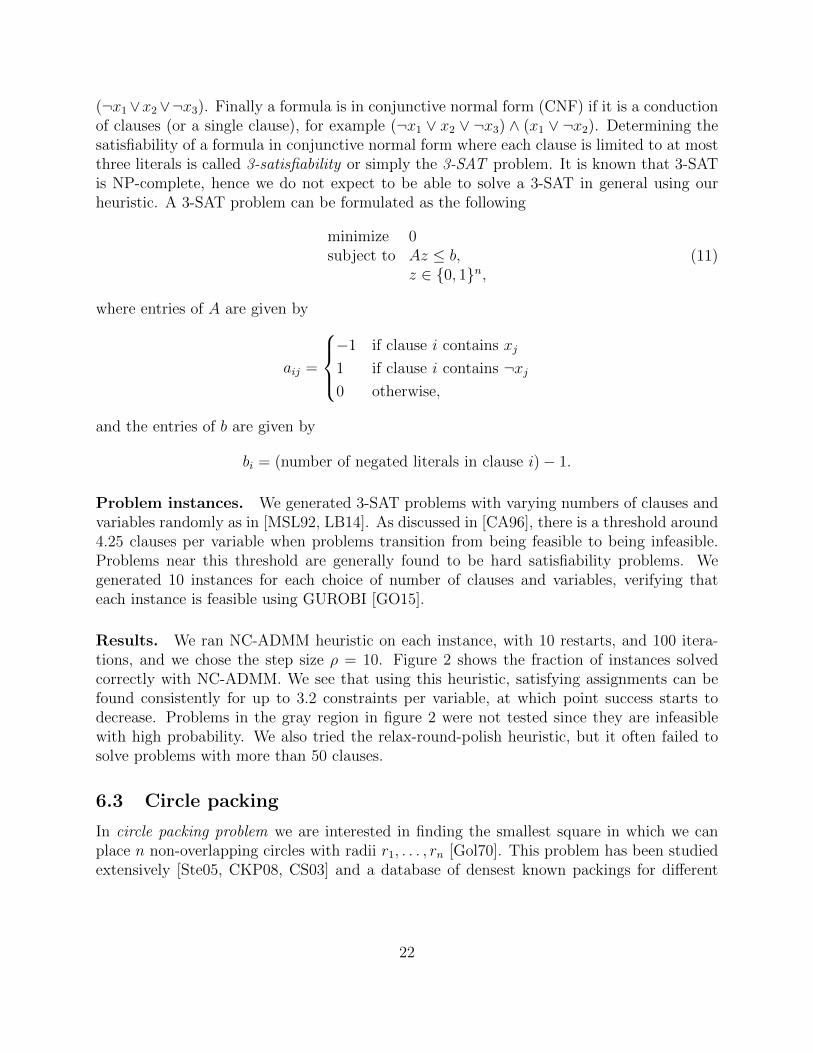
Results. We ran NC-ADMM heuristic on each instance, with 10 restarts, and 100 itera-tions, and we chose the step size ρ = 10. Figure 2 shows the fraction of instances solvedcorrectly with NC-ADMM. We see that using this heuristic, satisfying assignments can befound consistently for up to 3.2 constraints per variable, at which point success starts todecrease. Problems in the gray region in figure 2 were not tested since they are infeasiblewith high probability. We also tried the relax-round-polish heuristic, but it often failed tosolve problems with more than 50 clauses.

6.3 Circle packing

In circle packing problem we are interested in finding the smallest square in which we canplace n non-overlapping circles with radii r1, . . . , rn [Gol70]. This problem has been studiedextensively [Ste05, CKP08, CS03] and a database of densest known packings for different

22

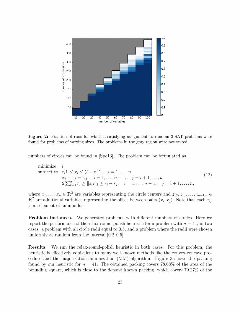
Figure 2: Fraction of runs for which a satisfying assignment to random 3-SAT problems werefound for problems of varying sizes. The problems in the gray region were not tested.

numbers of circles can be found in [Spe13]. The problem can be formulated as

minimize lsubject to ri1 ≤ xi ≤ (l − ri)1, i = 1, . . . , n

xi − xj = zij, i = 1, . . . , n− 1, j = i+ 1, . . . , n2∑n

k=1 ri ≥ ‖zij‖2 ≥ ri + rj, i = 1, . . . , n− 1, j = i+ 1, . . . , n,

(12)

where x1, . . . , xn ∈ R2 are variables representing the circle centers and z12, z13, . . . , zn−1,n ∈R2 are additional variables representing the offset between pairs (xi, xj). Note that each zijis an element of an annulus.

Problem instances. We generated problems with different numbers of circles. Here wereport the performance of the relax-round-polish heuristic for a problem with n = 41, in twocases: a problem with all circle radii equal to 0.5, and a problem where the radii were chosenuniformly at random from the interval [0.2, 0.5].

Results. We run the relax-round-polish heuristic in both cases. For this problem, theheuristic is effectively equivalent to many well-known methods like the convex-concave pro-cedure and the majorization-minimization (MM) algorithm. Figure 3 shows the packingfound by our heuristic for n = 41. The obtained packing covers 78.68% of the area of thebounding square, which is close to the densest known packing, which covers 79.27% of the

23

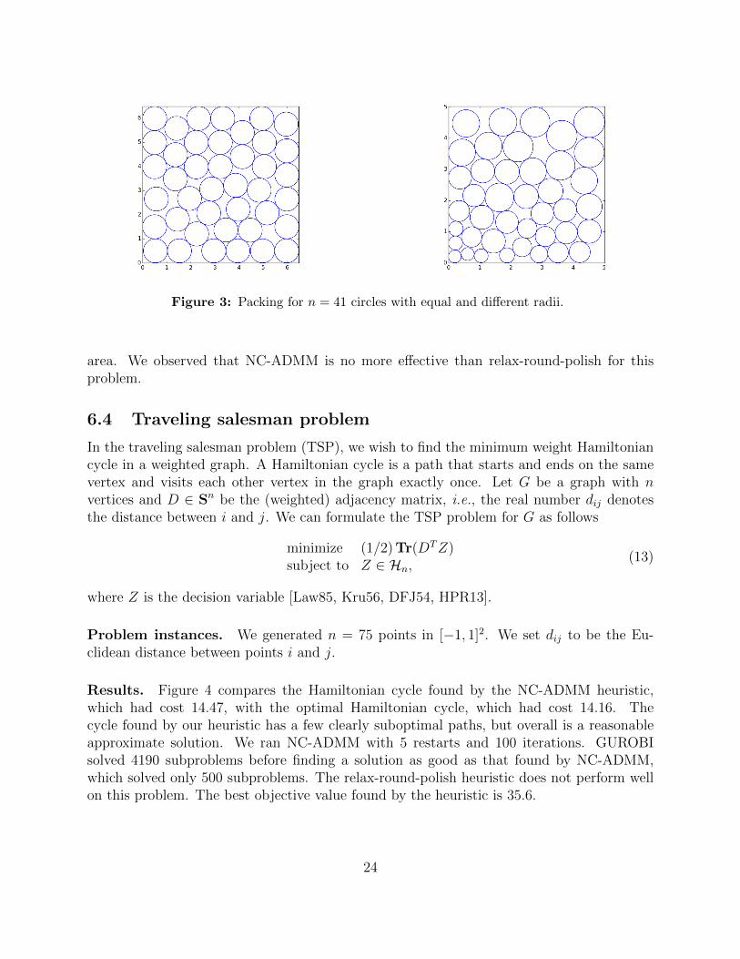
Figure 3: Packing for n = 41 circles with equal and different radii.

area. We observed that NC-ADMM is no more effective than relax-round-polish for thisproblem.

6.4 Traveling salesman problem

In the traveling salesman problem (TSP), we wish to find the minimum weight Hamiltoniancycle in a weighted graph. A Hamiltonian cycle is a path that starts and ends on the samevertex and visits each other vertex in the graph exactly once. Let G be a graph with nvertices and D ∈ Sn be the (weighted) adjacency matrix, i.e., the real number dij denotesthe distance between i and j. We can formulate the TSP problem for G as follows

minimize (1/2) Tr(DTZ)subject to Z ∈ Hn,

(13)

where Z is the decision variable [Law85, Kru56, DFJ54, HPR13].

Problem instances. We generated n = 75 points in [−1, 1]2. We set dij to be the Eu-clidean distance between points i and j.

Results. Figure 4 compares the Hamiltonian cycle found by the NC-ADMM heuristic,which had cost 14.47, with the optimal Hamiltonian cycle, which had cost 14.16. Thecycle found by our heuristic has a few clearly suboptimal paths, but overall is a reasonableapproximate solution. We ran NC-ADMM with 5 restarts and 100 iterations. GUROBIsolved 4190 subproblems before finding a solution as good as that found by NC-ADMM,which solved only 500 subproblems. The relax-round-polish heuristic does not perform wellon this problem. The best objective value found by the heuristic is 35.6.

24

Figure 4: Left: Hamiltonian cycle found by NC-ADMM. Right: optimal Hamiltonian cycle, foundusing GUROBI.

6.5 Factor analysis model

The factor analysis problem decomposes a matrix as a sum of a low-rank and a diagonalmatrix and has been studied extensively (for example in [SCPW12, NTGTB15]). It is alsoknown as the Frisch scheme in the system identification literature [Kal85, DM93]. Theproblem is the following

minimize ‖Σ− Σlr −D‖2F

subject to D = diag(d), d ≥ 0Σlr � 0Rank(Σlr) ≤ k,

(14)

where Σlr ∈ Sn+ and diagonal matrix D ∈ Rn×n with nonnegative diagonal entries are thedecision variables, and Σ ∈ Sn+ and k ∈ Z+ are problem data. One well-known heuristicfor solving this problem is adding ‖ · ‖∗, or nuclear norm, regularization and minimizing‖Σ−Σlr −D‖2

F + λ‖Σlr‖∗. The value of λ is chosen as the smallest value possible such thatRank(Σlr) ≤ k. Since Σlr is positive semidefinite, ‖Σlr‖∗ = Tr(Σlr).

Problem instances. We set k = bn/2c and generated the matrix F ∈ Rn×k by drawingthe entries i.i.d. from a standard normal distribution. We generated a diagonal matrix Dwith diagonal entries drawn i.i.d. from an exponential distribution with mean 1. We setΣ = FF T + D + V , where V ∈ Rn×n is a noise matrix with entries drawn i.i.d. fromN (0, σ2). We set σ2 = ‖FF T + diag(d)‖2

F/(400n2) so that the signal-to-noise ratio was near20.

Results. Figure 5 compares the average sum of squares error for the Σlr and d valuesfound by NC-ADMM, relax-round-polish, and the nuclear norm heuristic over 50 instances

25

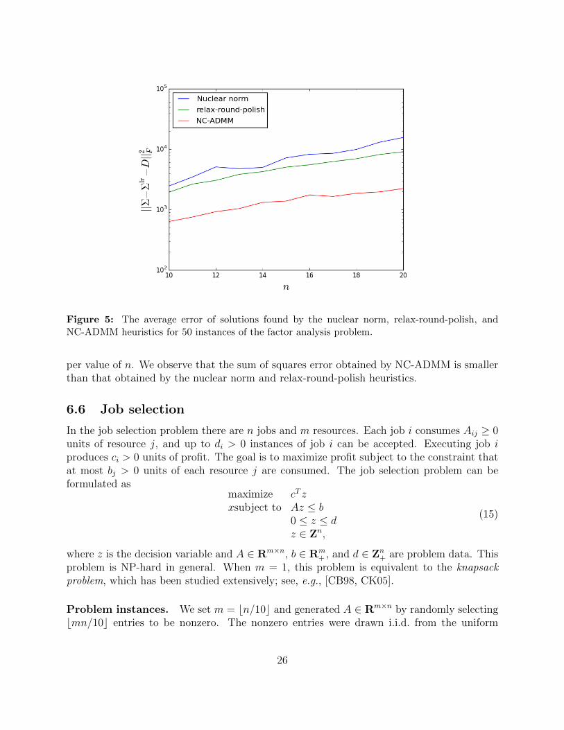
Figure 5: The average error of solutions found by the nuclear norm, relax-round-polish, andNC-ADMM heuristics for 50 instances of the factor analysis problem.

per value of n. We observe that the sum of squares error obtained by NC-ADMM is smallerthan that obtained by the nuclear norm and relax-round-polish heuristics.

6.6 Job selection

In the job selection problem there are n jobs and m resources. Each job i consumes Aij ≥ 0units of resource j, and up to di > 0 instances of job i can be accepted. Executing job iproduces ci > 0 units of profit. The goal is to maximize profit subject to the constraint thatat most bj > 0 units of each resource j are consumed. The job selection problem can beformulated as

maximize cT zxsubject to Az ≤ b

0 ≤ z ≤ dz ∈ Zn,

(15)

where z is the decision variable and A ∈ Rm×n, b ∈ Rm+ , and d ∈ Zn

+ are problem data. Thisproblem is NP-hard in general. When m = 1, this problem is equivalent to the knapsackproblem, which has been studied extensively; see, e.g., [CB98, CK05].

Problem instances. We set m = bn/10c and generated A ∈ Rm×n by randomly selectingbmn/10c entries to be nonzero. The nonzero entries were drawn i.i.d. from the uniform

26

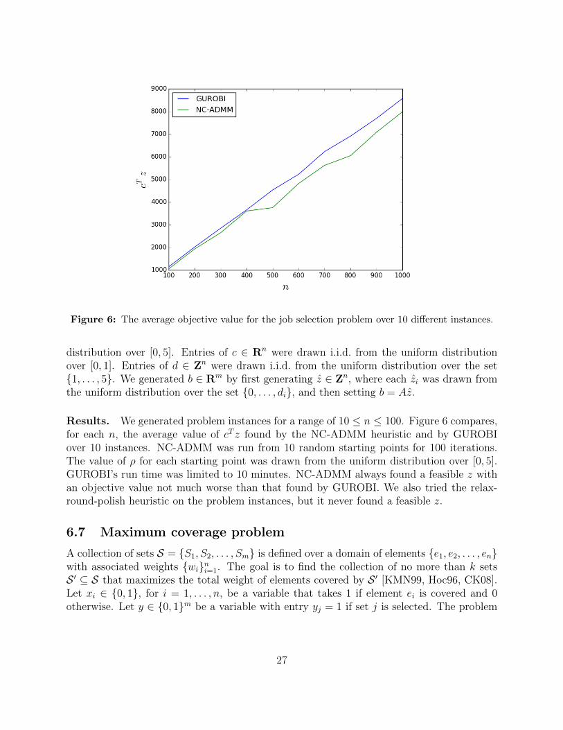
Figure 6: The average objective value for the job selection problem over 10 different instances.

distribution over [0, 5]. Entries of c ∈ Rn were drawn i.i.d. from the uniform distributionover [0, 1]. Entries of d ∈ Zn were drawn i.i.d. from the uniform distribution over the set{1, . . . , 5}. We generated b ∈ Rm by first generating z ∈ Zn, where each zi was drawn fromthe uniform distribution over the set {0, . . . , di}, and then setting b = Az.

Results. We generated problem instances for a range of 10 ≤ n ≤ 100. Figure 6 compares,for each n, the average value of cT z found by the NC-ADMM heuristic and by GUROBIover 10 instances. NC-ADMM was run from 10 random starting points for 100 iterations.The value of ρ for each starting point was drawn from the uniform distribution over [0, 5].GUROBI’s run time was limited to 10 minutes. NC-ADMM always found a feasible z withan objective value not much worse than that found by GUROBI. We also tried the relax-round-polish heuristic on the problem instances, but it never found a feasible z.

6.7 Maximum coverage problem

A collection of sets S = {S1, S2, . . . , Sm} is defined over a domain of elements {e1, e2, . . . , en}with associated weights {wi}ni=1. The goal is to find the collection of no more than k setsS ′ ⊆ S that maximizes the total weight of elements covered by S ′ [KMN99, Hoc96, CK08].Let xi ∈ {0, 1}, for i = 1, . . . , n, be a variable that takes 1 if element ei is covered and 0otherwise. Let y ∈ {0, 1}m be a variable with entry yj = 1 if set j is selected. The problem

27

Figure 7: The average solution weight over 10 different instances.

ismaximize wTxsubject to

∑j∈Sj

yj ≥ xi, i = 1, . . . , n

xi ∈ {0, 1}, i = 1, . . . , ny ∈ {0, 1}mcard(y) = k.

(16)

Note that y is a Boolean vector with fixed cardinality.

Problem instances. We generated problems as follows. Each set contained each of theelements independently with a constant probability p. Hence the expected size of each setwas np. There were m = 3/p sets, so the expected total number of elements in all sets (withrepetition) was equal to mnp = 3n. We set k = 1/(3p). Each wi was chosen uniformly atrandom from the interval [0, 1].

Results. We generated problems as described above for n = 50, 60, . . . , 240 and p = 0.01.For each value of n, we generated 10 problems and recorded the average weight wTx of theapproximate solutions found by NC-ADMM and the optimal solutions found by GUROBI.Figure 7 shows the results of our comparison of NC-ADMM and GUROBI. Approximatesolutions found by the relax-round-polish heuristic were far worse than those found by NC-ADMM for this problem.

28

6.8 Inexact graph isomorphism

Two (undirected) graphs are isomorphic if we can permute the vertices of one so it is thesame as the other (i.e., the same pairs of vertices are connected by edges). If we describethem by their adjacency matrices A and B, isomorphism is equivalent to the existence of apermutation matrix Z ∈ Rn×n such that ZAZT = B, or equivalently ZA = BZ.

Since in practical applications isomorphic graphs might be contaminated by noise, theinexact graph isomorphism problem is usually stated [ABK14, Ume88, CWH97], in which wewant to find a permutation matrix Z such that the disagreement ‖ZAZT −B‖2

F between thetransformed matrix and the target matrix is minimized. Since ‖ZAZT−B‖2

F = ‖ZA−BZ‖2F

for any permutation matrix Z, the inexact graph isomorphism problem can be formulatedas

minimize ‖ZA−BZ‖2F

subject to Z ∈ Pn.(17)

If the optimal value of this problem is zero, it means that A and B are isomorphic. Otherwise,the solution of this problem minimizes the disagreement of ZAZT and B in the Frobeniusnorm sense.

Solving inexact graph isomorphism problems is of interest in pattern recognition [CFSV04,RP94], computer vision [SRS01], shape analysis [SKK04, HHW06], image and video indexing[Lee06], and neuroscience [VCP+11]. In many of the aforementioned fields graphs are usedto represent geometric structures, and ‖ZAZT − B‖2

F can be interpreted as the strength ofgeometric deformation.

Problem instances. It can be shown that if A and B are isomorphic and A has distincteigenvalues and for all eigenvectors v of A for which 1Tv 6= 0, then the relaxed problem hasa unique solution which is the permutation matrix that relates A and B [ABK14]. Hence,in order to generate harder problems, we generated the matrix A such that it violatedthese conditions. In particular, we constructed A for the Peterson graph (3-regular with10 vertices), icosahedral graph (5-regular with 12 vertices), Ramsey graph (8-regular with17 vertices), dodecahedral graph (3-regular with 20 vertices), and the Tutte-Coxeter graph(3-regular with 30 vertices). For each example we randomly permuted the vertices to obtaintwo isomorphic graphs.

Results. We ran NC-ADMM with 20 iterations and 5 restarts. For all of our examplesNC-ADMM was able to find the permutation relating the two graphs. It is interesting tonotice that running the algorithm multiple times can find different solutions if there is morethan one permutation relating the two graphs. The relax-round-polish heuristic failed tofind a solution for all of the aforementioned problems.

29

7 Conclusions

We have discussed the relax-round-polish and NC-ADMM heuristics and demonstrated theirperformance on many different problems with convex objectives and decision variables froma nonconvex set. Our heuristics are easy to extend to additional problems because theyrely on a simple mathematical interface for nonconvex sets. We need only know a methodfor (approximate) projection onto the set. We do not require but benefit from knowing aconvex relaxation of the set, a convex restriction at any point in the set, and the neighborsof any point in the set under some discrete distance metric. Adapting our heuristics to anyparticular problem is straightforward, and we have fully automated the process in the NCVXpackage.

We do not claim that our heuristics give state-of-the-art results for any particular prob-lem. Rather, the purpose of our heuristics is to give a fast and reasonable solution withminimal tuning for a wide variety of problems. Our heuristics also take advantage of thetremendous progress in technology for solving general convex optimization problems, whichmakes it practical to treat solving a convex problem as a black box.

30

References

[ABK14] Y. Aflalo, A. Bronstein, and R. Kimmel. Graph matching: relax or not? arXivpreprint arXiv:1401.7623, 2014.

[ABK15] Y. Aflalo, A. Bronstein, and R. Kimmel. On convex relaxation of graph isomor-phism. Proceedings of the National Academy of Sciences, 112(10):2942–2947,2015.

[Ach09] T. Achterberg. SCIP: solving constraint integer programs. Mathematical Pro-gramming Computation, 1(1):1–41, 2009.

[AM85] W. N. Anderson and T. D. Morley. Eigenvalues of the Laplacian of a graph.Linear and Multilinear Algebra, 18(2):141–145, 1985.

[ApS15] MOSEK ApS. The MOSEK optimization toolbox for MATLAB manual. Ver-sion 7.1 (Revision 28), 2015.

[BBC+08] P. Bonami, L. T. Biegler, A. R. Conn, G. Cornuejols, I. E. Grossmann, C. D.Laird, J. Lee, A. Lodi, F. Margot, and N. Sawaya. An algorithmic framework forconvex mixed integer nonlinear programs. Discrete Optimization, 5(2):186–204,2008.

[Bec14] A. Beck. Introduction to Nonlinear Optimization: Theory, Algorithms, andApplications with MATLAB, volume 19. SIAM, 2014.

[Bel09] P. Belotti. Couenne: a user’s manual. Technical Report, 2009.

[Bem15] A. Bemporad. Solving mixed-integer quadratic programs via nonnegative leastsquares. 5th IFAC Conference on Nonlinear Model Predictive Control, pages73–79, 2015.

[Ber14] D. P. Bertsekas. Constrained optimization and Lagrange multiplier methods.Academic press, 2014.

[BHA15] S. Boyd, M. Hast, and K. J. Astrom. MIMO PID tuning via iterated LMIrestriction. International Journal of Robust and Nonlinear Control, 2015.

[BJS94] P. Brucker, B. Jurisch, and B. Sievers. A branch and bound algorithm forthe job-shop scheduling problem. Discrete applied mathematics, 49(1):107–127,1994.

[BM99] A. Bemporad and M. Morari. Control of systems integrating logic, dynamics,and constraints. Automatica, 35(3):407–427, 1999.

[BNW06] R. H. Byrd, J. Nocedal, and R. A. Waltz. Knitro: An integrated package fornonlinear optimization. In Large-scale nonlinear optimization, pages 35–59.Springer, 2006.

31

[Bol13] D. Boley. Local linear convergence of the alternating direction method ofmultipliers on quadratic or linear programs. SIAM Journal on Optimization,23(4):2183–2207, 2013.

[BP12] A. Bemporad and P. Patrinos. Simple and certifiable quadratic programmingalgorithms for embedded linear model predictive control. In Nonlinear ModelPredictive Control, volume 4, pages 14–20, 2012.

[BPC+11] S. Boyd, N. Parikh, E. Chu, B. Peleato, and J. Eckstein. Distributed optimiza-tion and statistical learning via the alternating direction method of multipliers.Foundations and Trends in Machine Learning, 3(1):1–122, 2011.

[Bra10] A. M. Bradley. Algorithms for the Equilibration of Matrices and their Ap-plication to Limited-Memory Quasi-Newton Methods. PhD thesis, StanfordUniversity, 2010.

[BRL01] A. Bemporad, J. Roll, and L. Ljung. Identification of hybrid systems via mixed-integer programming. In IEEE Conference on Decision and Control, volume 1,pages 786–792, 2001.

[BV04] S. Boyd and L. Vandenberghe. Convex Optimization. Cambridge UniversityPress, 2004.

[CA96] J. M. Crawford and L. D. Auton. Experimental results on the crossover pointin random 3-SAT. Artificial intelligence, 81(1):31–57, 1996.

[CA06] M. Carrion and J. M. Arroyo. A computationally efficient mixed-integer linearformulation for the thermal unit commitment problem. IEEE Transactions onPower Systems, 21(3):1371–1378, 2006.

[CB98] P. C. Chu and J. E. Beasley. A genetic algorithm for the multidimensionalknapsack problem. Journal of heuristics, 4(1):63–86, 1998.

[CFSV04] D. Conte, P. Foggia, C. Sansone, and M. Vento. Thirty years of graph matchingin pattern recognition. International journal of pattern recognition and artificialintelligence, 18(03):265–298, 2004.

[Cha12] R. Chartrand. Nonconvex splitting for regularized low-rank + sparse decom-position. IEEE Transactions on Signal Processing, 60(11):5810–5819, 2012.

[CK05] C. Chekuri and S. Khanna. A polynomial time approximation scheme for themultiple knapsack problem. SIAM Journal on Computing, 35(3):713–728, 2005.

[CK08] R. Cohen and L. Katzir. The generalized maximum coverage problem. Infor-mation Processing Letters, 108(1):15–22, 2008.

32

[CKP08] I. Castillo, F. J. Kampas, and J. D. Pinter. Solving circle packing problems byglobal optimization: numerical results and industrial applications. EuropeanJournal of Operational Research, 191(3):786–802, 2008.

[CPDB13] E. Chu, N. Parikh, A. Domahidi, and S. Boyd. Code generation for embeddedsecond-order cone programming. In Proceedings of the 2013 European ControlConference, pages 1547–1552, 2013.

[CPL09] IBM ILOG CPLEX. User’s manual for CPLEX, version 12.1. InternationalBusiness Machines Corporation, 46(53):157, 2009.

[CPM10] J. P. S. Catalao, H. M. I. Pousinho, and V. M. F. Mendes. Scheduling ofhead-dependent cascaded hydro systems: Mixed-integer quadratic program-ming approach. Energy Conversion and Management, 51(3):524–530, 2010.

[CS03] C. R. Collins and K. Stephenson. A circle packing algorithm. ComputationalGeometry, 25(3):233–256, 2003.

[CW13] R. Chartrand and B. Wohlberg. A nonconvex ADMM algorithm for groupsparsity with sparse groups. In Proceedings of IEEE International Conferenceon Acoustics, Speech and Signal Processing (ICASSP), pages 6009–6013. IEEE,2013.

[CWH97] A. D. J. Cross, R. C. Wilson, and E. R. Hancock. Inexact graph matchingusing genetic search. Pattern Recognition, 30(6):953–970, 1997.

[DBEY13] N. Derbinsky, J. Bento, V. Elser, and J. S. Yedidia. An improved three-weightmessage-passing algorithm. arXiv:1305.1961 [cs.AI], 2013.

[DCB13] A. Domahidi, E. Chu, and S. Boyd. ECOS: An SOCP solver for embeddedsystems. In Proceedings of the 12th European Control Conference, pages 3071–3076. IEEE, 2013.

[DCB14] S. Diamond, E. Chu, and S. Boyd. CVXPY: A Python-embedded modelinglanguage for convex optimization, version 0.2. http://cvxpy.org/, May 2014.

[DFJ54] G. Dantzig, R. Fulkerson, and S. Johnson. Solution of a large-scale traveling-salesman problem. Journal of the operations research society of America,2(4):393–410, 1954.

[DM93] J. David and B. De Moor. The opposite of analytic centering for solving min-imum rank problems in control and identification. In Proceedings of the 32ndIEEE Conference on Decision and Control, pages 2901–2902. IEEE, 1993.

[EB92] J. Eckstein and D. P. Bertsekas. On the Douglas-Rachford splitting method andthe proximal point algorithm for maximal monotone operators. MathematicalProgramming, 55(1-3):293–318, 1992.

33

[Ers14] T. Erseghe. Distributed optimal power flow using ADMM. IEEE Transactionson Power Systems, 29(5):2370–2380, 2014.

[FDM15] D. Frick, A. Domahidi, and M. Morari. Embedded optimization for mixedlogical dynamical systems. Computers and Chemical Engineering, 72:21–33,2015.

[FHT01] J. Friedman, T. Hastie, and R. Tibshirani. The elements of statistical learning,volume 1. Springer series in statistics Springer, Berlin, 2001.

[Fle73] R. Fletcher. An exact penalty function for nonlinear programming with in-equalities. Mathematical Programming, 5(1):129–150, 1973.

[Flo95] C. A. Floudas. Nonlinear and Mixed-Integer Optimization: Fundamentals andApplications. Oxford University Press, 1995.

[GB14a] P. Giselsson and S. Boyd. Diagonal scaling in Douglas-Rachford splitting andADMM. In 53rd Annual IEEE Conference on Decision and Control (CDC),pages 5033–5039, 2014.

[GB14b] P. Giselsson and S. Boyd. Monotonicity and restart in fast gradient methods.In 53rd Annual IEEE Conference on Decision and Control (CDC), pages 5058–5063, 2014.

[GB14c] P. Giselsson and S. Boyd. Preconditioning in fast dual gradient methods. In53rd Annual IEEE Conference on Decision and Control (CDC), pages 5040–5045, 2014.

[GM12] S. Gualandi and F. Malucelli. Exact solution of graph coloring problems viaconstraint programming and column generation. INFORMS Journal on Com-puting, 24(1):81–100, 2012.

[GO15] Inc. Gurobi Optimization. Gurobi Optimizer Reference Manual, 2015.

[Gol70] M. Goldberg. The packing of equal circles in a square. Mathematics Magazine,pages 24–30, 1970.

[Gro07] J. L. Gross. Combinatorial methods with computer applications. CRC Press,2007.

[GTSJ15] E. Ghadimi, A. Teixeira, I. Shames, and M. Johansson. Optimal parameter se-lection for the alternating direction method of multipliers (ADMM): Quadraticproblems. IEEE Transactions on Automatic Control, 60(3):644–658, 2015.

[Hes69] M. R. Hestenes. Multiplier and gradient methods. Journal of optimizationtheory and applications, 4(5):303–320, 1969.

34

[HHW06] L. He, C. Y. Han, and W. G. Wee. Object recognition and recovery by skeletongraph matching. In IEEE International Conference on Multimedia and Expo,pages 993–996. IEEE, 2006.

[HL12] M. Hong and Z. Luo. On the linear convergence of the alternating directionmethod of multipliers. arXiv preprint arXiv:1208.3922, 2012.

[HLR14] M. Hong, Z. Luo, and M. Razaviyayn. Convergence analysis of alternatingdirection method of multipliers for a family of nonconvex problems. arXivpreprint arXiv:1410.1390, 2014.

[HM79] S. P. Han and O. L. Mangasarian. Exact penalty functions in nonlinear pro-gramming. Mathematical programming, 17(1):251–269, 1979.

[Hma10] H. Hmam. Quadratic optimization with one quadratic equality constraint.Technical report, Electronic Warfare and Radar Division, Defence Science andTechnology Organisation (DSTO), Australia, 2010.

[Hoc96] D. S. Hochbaum. Approximating covering and packing problems: set cover, ver-tex cover, independent set, and related problems. In Approximation algorithmsfor NP-hard problems, pages 94–143. PWS Publishing Co., 1996.

[Hon14] M. Hong. A distributed, asynchronous and incremental algorithm for nonconvexoptimization: An ADMM based approach. arXiv preprint arXiv:1412.6058,2014.

[HPR13] K. L. Hoffman, M. Padberg, and G. Rinaldi. Traveling salesman problem. InEncyclopedia of Operations Research and Management Science, pages 1573–1578. Springer, 2013.

[HS16] K. Huang and N. D. Sidiropoulos. Consensus-ADMM for general quadraticallyconstrained quadratic programming. arXiv preprint arXiv:1601.02335, 2016.

[JGR+14] J. L. Jerez, P. J. Goulart, S. Richter, G. Constantinides, E. C. Kerrigan,M. Morari, et al. Embedded online optimization for model predictive control atmegahertz rates. IEEE Transactions on Automatic Control, 59(12):3238–3251,2014.

[JMZ14] B. Jiang, S. Ma, and S. Zhang. Alternating direction method of multipliers forreal and complex polynomial optimization models. Optimization, 63(6):883–898, 2014.

[Joh14] S. G. Johnson. The NLopt nonlinear-optimization package, 2014.

[Kal85] R. E. Kalman. Identification of noisy systems. Russian Mathematical Surveys,40(4):25–42, 1985.

35

[KMN99] S. Khuller, A. Moss, and J. S. Naor. The budgeted maximum coverage problem.Information Processing Letters, 70(1):39–45, 1999.

[Kru56] J. B. Kruskal. On the shortest spanning subtree of a graph and the travelingsalesman problem. Proceedings of the American Mathematical society, 7(1):48–50, 1956.

[Kuh05] H. W. Kuhn. The hungarian method for the assignment problem. Naval Re-search Logistics (NRL), 52(1):7–21, 2005.

[Law85] E. L. Lawler. The traveling salesman problem: a guided tour of combinatorialoptimization. Wiley Series in Discrete Mathematics, 1985.

[LB14] T. Lipp and S. Boyd. Variations and extensions of the convex-concave proce-dure, 2014.

[Lee06] J. Lee. A graph-based approach for modeling and indexing video data. In IEEEInternational Symposium on Multimedia, pages 348–355. IEEE, 2006.

[LP14] G. Li and T. K. Pong. Splitting methods for nonconvex composite optimization.arXiv preprint arXiv:1407.0753, 2014.

[LP15] G. Li and T. K. Pong. Global convergence of splitting methods for nonconvexcomposite optimization. arXiv e-Print 1407.0753, 2015.

[LS14] A. P. Liavas and N. D. Sidiropoulos. Parallel algorithms for constrained tensorfactorization via the alternating direction method of multipliers. arXiv preprintarXiv:1409.2383, 2014.

[LW66] E. L. Lawler and D. E. Wood. Branch-and-bound methods: A survey. Opera-tions research, 14(4):699–719, 1966.

[MB10] J. Mattingley and S. Boyd. Automatic code generation for real-time convexoptimization. Convex Optimization in Signal Processing and Communications,pages 1–41, 2010.

[MB12] J. Mattingley and S. Boyd. CVXGEN: a code generator for embedded convexoptimization. Optimization and Engineering, 13(1):1–27, 2012.

[Mer94] R. Merris. Laplacian matrices of graphs: a survey. Linear algebra and itsapplications, 197:143–176, 1994.

[MSL92] D. Mitchell, B. Selman, and H. Levesque. Hard and easy distributions of SATproblems. In AAAI, volume 92, pages 459–465, 1992.

[MWB11] J. Mattingley, Y. Wang, and S. Boyd. Receding horizon control: Automaticgeneration of high-speed solvers. IEEE Control Systems Magazine, 31(3):52–65,2011.

36

[Neu37] J. Von Neumann. Some matrix inequalities and metrization of metric space.Tomsk University Review, 1:286–296, 1937.

[NF77] P. M. Narendra and K. Fukunaga. A branch and bound algorithm for featuresubset selection. IEEE Transactions on Computers, 100(9):917–922, 1977.

[NTGTB15] L. Ning, T. Tryphon T. Georgiou, A. Tannenbaum, and S. Boyd. Linear modelsbased on noisy data and the frisch scheme. SIAM Review, 57(2):167–197, 2015.

[OSB13] B. O’Donoghue, G. Stathopoulos, and S. Boyd. A splitting method for optimalcontrol. IEEE Transactions on Control Systems Technology, 21(6):2432–2442,2013.

[PB13] N. Parikh and S. Boyd. Proximal algorithms. Foundations and Trends inOptimization, 1(3):123–231, 2013.

[PB14] N. Parikh and S. Boyd. Block splitting for distributed optimization. Mathe-matical Programming Computation, 6(1):77–102, 2014.

[PCZ15] Z. Peng, J. Chen, and W. Zhu. A proximal alternating direction method ofmultipliers for a minimization problem with nonconvex constraints. Journal ofGlobal Optimization, pages 1–18, 2015.

[PF07] L. G. Papageorgiou and E. S. Fraga. A mixed integer quadratic programmingformulation for the economic dispatch of generators with prohibited operatingzones. Electric power systems research, 77(10):1292–1296, 2007.

[PG89] G. Di Pillo and L. Grippo. Exact penalty functions in constrained optimization.SIAM Journal on control and optimization, 27(6):1333–1360, 1989.

[PR91] M. Padberg and G. Rinaldi. A branch-and-cut algorithm for the resolution oflarge-scale symmetric traveling salesman problems. SIAM review, 33(1):60–100,1991.

[RP94] J. Rocha and T. Pavlidis. A shape analysis model with applications to a char-acter recognition system. IEEE Transactions on Pattern Analysis and MachineIntelligence, 16(4):393–404, 1994.

[SA90] H. D. Sherali and W. P. Adams. A hierarchy of relaxations between the con-tinuous and convex hull representations for zero-one programming problems.SIAM Journal on Discrete Mathematics, 3(3):411–430, 1990.

[SCPW12] J. Saunderson, V. Chandrasekaran, P. A. Parrilo, and A. S. Willsky. Diagonaland low-rank matrix decompositions, correlation matrices, and ellipsoid fitting.SIAM Journal on Matrix Analysis and Applications, 33(4):1395–1416, 2012.

37

[SKK04] T. B. Sebastian, P. N. Klein, and B. B. Kimia. Recognition of shapes by edit-ing their shock graphs. IEEE Transactions on Pattern Analysis and MachineIntelligence, 26(5):550–571, 2004.

[Slu69] A. V. D. Sluis. Condition numbers and equilibration of matrices. NumerischeMathematik, 14(1):14–23, 1969.

[SLY+14] W. Shi, Q. Ling, K. Yuan, G. Wu, and W. Yin. On the linear convergenceof the admm in decentralized consensus optimization. IEEE Transactions onSignal Processing, 62(7):1750–1761, 2014.

[SM99] R. A. Stubbs and S. Mehrotra. A branch-and-cut method for 0-1 mixed convexprogramming. Mathematical programming, 86(3):515–532, 1999.

[SP14] S.You and Q. Peng. A non-convex alternating direction method of multipliersheuristic for optimal power flow. In 2014 IEEE International Conference onSmart Grid Communications (SmartGridComm), pages 788–793. IEEE, 2014.

[Spe13] E. Specht. Packomania. http://www.packomania.com/, October 2013.

[Spi85] J. E. Spingarn. Applications of the method of partial inverses to convex pro-gramming: decomposition. Mathematical Programming, 32(2):199–223, 1985.

[SRS01] C. Schellewald, S. Roth, and C. Schnorr. Evaluation of convex optimizationtechniques for the weighted graph-matching problem in computer vision. InPattern Recognition, pages 361–368. Springer, 2001.

[Ste05] K. Stephenson. Introduction to circle packing: The theory of discrete analyticfunctions. Cambridge University Press, 2005.

[TMBB15] R. Takapoui, N. Moehle, S. Boyd, and A. Bemporad. A simple effectiveheuristic for embedded mixed-integer quadratic programming. arXiv preprintarXiv:1509.08416, 2015.

[TS05a] M. Tawarmalani and N. V. Sahinidis. A polyhedral branch-and-cut approachto global optimization. Mathematical Programming, 103:225–249, 2005.

[TS05b] M. Tawarmalani and N. V. Sahinidis. A polyhedral branch-and-cut approachto global optimization. Mathematical Programming, 103(2):225–249, 2005.

[Ull11] F. Ullmann. FiOrdOs: A Matlab toolbox for C-code generation for first ordermethods. Master’s thesis, ETH Zurich, 2011.

[Ume88] S. Umeyama. An eigendecomposition approach to weighted graph matchingproblems. IEEE Transactions on Pattern Analysis and Machine Intelligence,10(5):695–703, 1988.

38

[VCP+11] J. T. Vogelstein, J. M. Conroy, L. J. Podrazik, S. G. Kratzer, E. T. Harley, D. E.Fishkind, R. J. Vogelstein, and C. E. Priebe. Large (brain) graph matchingvia fast approximate quadratic programming. arXiv preprint arXiv:1112.5507,2011.

[WB10] Y. Wang and S. Boyd. Fast model predictive control using online optimization.IEEE Transactions on Control Systems Technology, 18(2):267–278, 2010.

[WLMK09] A. Waechter, C. Lairdl, F. Margot, and Y. Kawajir. Introduction to IPOPT:A tutorial for downloading, installing, and using IPOPT, 2009.

[WN99] S. J. Wright and J. Nocedal. Numerical Optimization, volume 2. Springer NewYork, 1999.

[WXX14] F. Wang, Z. Xu, and H. Xu. Convergence of alternating directionmethod with multipliers for non-convex composite problems. arXiv preprintarXiv:1410.8625, 2014.

[XYWZ12] Y. Xu, W. Yin, Z. Wen, and Y. Zhang. An alternating direction algorithmfor matrix completion with nonnegative factors. Frontiers of Mathematics inChina, 7(2):365–384, 2012.

39