a general adaptive solver for hyperbolic pdes based on filter bank subdivisions

Applied Numerical Mathematics 33 (2000) 317–325

A general adaptive solver for hyperbolic PDEs based onfilter bank subdivisions

Johan Waldén1

Yale University, Department of Mathematics, 10 Hillhouse Avenue, P.O. Box 208283, New Haven, CT 06520, USA

Abstract

We use the filter bank method to solve hyperbolic PDEs adaptively. We show that the method is well-suitedfor object-oriented design. We also test the robustness and computational speed of the method, and it is shownto outperform nonadaptive schemes even for small problem sizes. 2000 IMACS. Published by Elsevier ScienceB.V. All rights reserved.

Keywords:Wavelets; Adaptive PDE methods; Filter banks; Numerical methods

1. Introduction

1.1. Background

The idea that the regularity of a function (in terms of its Hölder exponent) is completely characterizedby the magnitude of the coefficients of its wavelet expansion [2] seems useful if we want to constructadaptive solvers for hyperbolic PDEs.

As the solutions of hyperbolic equations often are smooth except for some small regions with sharpgradients (or even discontinuities in the nonviscous case), and the wavelet coefficients only depend onthe local regularity of a function, we can expect such a solution to have a sparse representation in awavelet basis, at least if we decide some threshold value below which we set coefficients to zero (socalledε-thresholding).

However, the straightforward implementation of such a sparse solver, using a Galerkin method, tendsto be inefficient as shown, e.g., in [1]. This is true especially for nonlinear equations, as multiplicationis nontrivial in the wavelet domain. The constants in the asymptotic complexity estimates are simply toolarge for numerical efficiency.

These difficulties inspired the development of thefilter bank method[3]. The idea is to “split”the solver into two parts:the operator part, for which finite difference approximations are used, and

1 E-mail: [email protected]

0168-9274/00/$20.00 2000 IMACS. Published by Elsevier Science B.V. All rights reserved.PII: S0168-9274(99)00098-7

318 J. Waldén / Applied Numerical Mathematics 33 (2000) 317–325

Fig. 1. Splitting of solver into two parts. The operator part and the representation part are independent. InterfacethroughΛ-cycles.

the representation partwhere the filter bank transform (which is the discrete version of the wavelettransform) is used. Ideally, the operator part of the solver would be constructed taking into considerationthe questions of stability and order of approximation and then the representation part, which is very muchthe same regardless of the problem, is “hooked onto the solver” to give adaptivity. The interface betweenthese two parts consists of so calledΛ-cycles. The idea is shown in Fig. 1.

This approach of splitting the solver, switching from the wavelet to the filter bank transform for therepresentation part and using finite difference methods for the operator part has a number of advantages.The most crucial are:• With the right filter banks, multiplication of functions becomes trivial.• Short filters that may not correspond to any wavelets can be used, leading to faster solvers, and less

extra work at boundaries.• The automatic scale decomposition and detection of sharp gradients make it simple to use different

solvers in different parts of the domain. We can, e.g., add viscosity terms in a neighborhood ofboundary layers. Furthermore, we can take larger time steps on coarser levels, which we will use inthis paper to increase the efficiency of the method.

A discrete version of the implication: local Hölder regularity⇒ local sparse representation was alsoderived in [3], which implies that by restricting ourselves to grids with dyadic structures, and using thefilter bank transform to go between different resolutions, we get a bound on the growth of the norms ofthe transforms as we increase the number of levels. This will lead to nice stability properties as we willsee.

The results presented in [3] were promising, but as we only dealt with periodic boundary conditions,and never measured the computational speed of the method, it was still “experimental”. The tests in thispaper were made for problems with boundary conditions (by using the boundary filter banks introducedin [4]), and we will compare the CPU time for the sparse and a nonsparse solver.

J. Waldén / Applied Numerical Mathematics 33 (2000) 317–325 319

Fig. 2. Applying the filter bank transform to a grid function. The function is smooth, except for in themiddle where it has a sharp gradient. (a) initial grid (squares represent grid points), (b) filter bank transformedmultilevel representation, (c) thresholded representation. (The squares are coefficients that are kept in the sparserepresentation.)

Fig. 3.Λ-cycle for fast differentiation of thresholded representation. Squares denote kept coefficients.

1.2. The filter bank method

We give a brief description of the filter bank method. The filter bank transform formally does thesame thing as the wavelet transform, but it works on discrete functions (grid functions) instead of onwavelet spaces. The transform decomposes a grid function into a multilevel representation. By requiringvanishing momentproperties of the filters involved in the transform, it is assured that we get a sparserepresentation when we do the thresholding, i.e.,ns� n wheren is the initial number of grid points andns is the number of coefficients in the thresholded expansion. The idea is shown in Fig. 2.

We need methods of complexity O(ns), that apply operators to a sparse representation. We do asfollows: We start on the coarsest level. For coefficients where there is no finer scale “above” (meaningthat there is no coefficient on a finer level which would influence the result if we transformed back tothe finer level) we apply the operator. For coefficients where thereare such coefficients, we transformone step backwards, and do the same procedure again. We do this recursively, back to the finest scale,and then start transforming forward, getting the coefficients from finer scales where they exist. The ideais shown in Fig. 3, in which the solid arrows represent the part when we go backwards, and the dashedarrows when we go forward. The coefficients lying between the dashed arrows will be fetched from finerlevels, and we apply the operator on the same level for the coefficients lying outside the dashed arrows.We call this total procedure aΛ-cycle.

We remark that theΛ-cycle will be the same regardless of the operator (although we might have toadd special conditions for the filters in the filter bank transform depending on the operator), and that theoperators work onuniformgrids although the total representation is nonuniform. This means that we canimplement them as if we are working with a nonadaptive method on a uniform grid, which permits us toseparate the solver into the representation part and the operator part.


We also remark that theΛ-cycle relies on the fact that for hyperbolic equations, things will not happen“too fast” (e.g., a shock will not travel more than a couple of points in each time step). Such restrictionsare already present by the CFL-condition.

For a detailed description of the filter bank transform, andΛ-cycles, we refer to [3].

1.3. Contents

We test the filter bank method. We are especially interested in answering the following questions:• How well separated are the operator and the representation problems? Is it “easy” to hook the filter

bank part onto an arbitrary problem? As the program is written in C++, this would capture theimportant object oriented properties of encapsulation and code reuse.• What is the break-even problem size between the adaptive method and the nonadaptive method

(i.e., the “pure” finite difference solver)? How far have we brought down the complexity constantsby using the filter bank method?• How robust is the method? Can we solve a large set of problems without having to fine-tune

parameters?

2. Implementation

The separation of the solver into different parts fits well into the framework of an object orientedprogramming language, and the solver has been implemented in C++.

Of course, the choice of representation of the thresholded expansion is crucial for the performanceof the sparse solver. In [3], a block linked list data structure was proposed for the representation of athresholded grid. By working with blocks of 8–32 coefficients we decrease the overhead involved inaccessing coefficients, thresholding, etc. Another choice would be to have a two level tree representation,where on the first level each element is a pointer to a block. A NULL pointer means that the block hasbeen thresholded. The different data structures are shown in Fig. 4.

If we compare the tree and the linked list data structure, there will be much less overhead involved infinding coefficients when using a tree structure. On the other hand, traversing a whole grid will be moreefficient for the linked list structure, which will also use less memory.

The asymptotic behavior of the tree structure will be the same as of the nonsparse solver (although,hopefully the constants involved will bemuchsmaller), as traversing a grid implemented with a treestructure is of complexity O(N), whereN is the number of blocks of thenonsparserepresentation. Thisis in contrast to the linked list representation where the operation is O(Ns), whereNs is the number ofblocks of thesparserepresentation. We would, therefore, expect that the solver with a tree structure willbe more efficient for small problem sizes, whereas for larger problem sizes, the linked list structure willbe more efficient. We have the same asymptotics from the memory point of view: O(N) for the treestructure and O(Ns) for the linked list structure.

We have implemented all three of these data structures. We show a class diagram over the classesused (Fig. 5). The virtual classLevelhas the childrenLevelGrid, LevelListandLevelTree. The operatorpart of the program works on these classes, and the classFiniteDifferenceStencilis a part of a generaloperator.


Fig. 4. Some possible representations of a level. (a) The nonsparse representation, which is simply to allocate allthe coefficients consecutively in memory. (b) The linked list representation where only significant blocks are kept.(c) A two level tree representation where NULL pointers correspond to thresholded blocks.

Fig. 5. Class diagram for filter bank solver.

A SparseExpansionconsists of a number ofLevels, and to this class we associate the filter bankoperations, which use the classesFilter and FilterBank. Furthermore, the thresholding operation is amember of this class.

3. Efficiency

We now compare a nonsparse and a sparse solver. We are especially interested in finding the break-evenbetween these two when it comes to CPU time and memory allocation. As a test problem, we choose theadvection equation{

ut = ux, 06 x 6 1, t > 0,u(x,0)= u0(x), u(1, t)= u0(t mod 1),

(1)

where

u0(x)= sin(2πx)+ e−α(x−0.5)2, α = 0.22n8/5, (2)


Fig. 6. CPU time for solving advection equation with different data structures and problem sizesn= 1024–32768.‘x’ = nonsparse solver, ‘◦’ = linked list data structure, ‘∗’ = tree data structure, ‘+’= tree data structure andvariable time steps.

as it is very simple, but still captures the essence of the filter bank method (we have tested the one-dimensional Euler’s equations with similar results). This equation is in some sense the worst case forthe nonsparse solver, as the operator is so easy to evaluate and the overhead of using the sparse solver isroughly constant.

In (2), n denotes the number of grid points (each block containing 16 points, son= 16N whereN isthe number ofblocks). The solution is a smooth function with a “spike” traveling to the left of the interval.We use a 4th finite difference scheme with one sided boundary stencils, the classical 4th order Runge–Kutta method for the time marching, and the 4th order boundary filter bank described in [4]. We varythe sharpness of the spike with the number of grid points, as otherwise we would resolve the spike whenincreasing the number of points and threshold all coefficients on fine levels. An analysis of the localtruncation error shows that we should chooseα ∝ n8/5 for a 4th order method.

The program was compiled with the -fast flag, and run on a SUN UltraSPARC. We compare the CPUtime for a nonsparse solver with the tree and linked list implementations of the sparse solver. The resultsare shown in Fig. 6. We see that the nonsparse solver behaves as O(n2). The break-even when using thelinked list solver lies between 8192 and 16384 points. This is improved by using the tree solver, whichhas a break-even between 4096 and 8192 points. The tree solver is O(n2) whereas the linked list solverideally would be O(n log(n)) (as ideally, we would havens∝ logn). However, for these problem sizesthis difference does not show, and the problem size needs to be large before the linked list structure willbeat the tree data structure. Furthermore, the tree structure is simpler to implement.

If we go one step further and use variable time steps (having a time step proportional to the spaceresolution on each level), we can bring down the break-even size even further, as shown in Fig. 6. Withthis solver the break-even size lies between 1024 and 2048 points. Asymptotically this could bring the


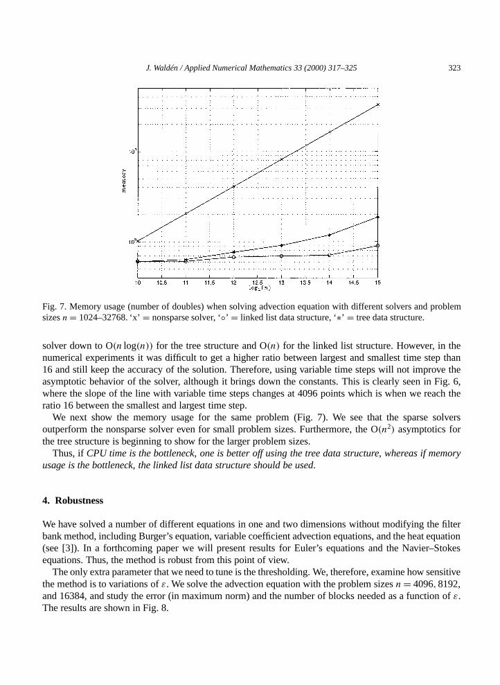
Fig. 7. Memory usage (number of doubles) when solving advection equation with different solvers and problemsizesn= 1024–32768. ‘x’= nonsparse solver, ‘◦’ = linked list data structure, ‘∗’ = tree data structure.

solver down to O(n log(n)) for the tree structure and O(n) for the linked list structure. However, in thenumerical experiments it was difficult to get a higher ratio between largest and smallest time step than16 and still keep the accuracy of the solution. Therefore, using variable time steps will not improve theasymptotic behavior of the solver, although it brings down the constants. This is clearly seen in Fig. 6,where the slope of the line with variable time steps changes at 4096 points which is when we reach theratio 16 between the smallest and largest time step.

We next show the memory usage for the same problem (Fig. 7). We see that the sparse solversoutperform the nonsparse solver even for small problem sizes. Furthermore, the O(n2) asymptotics forthe tree structure is beginning to show for the larger problem sizes.

Thus, ifCPU time is the bottleneck, one is better off using the tree data structure, whereas if memoryusage is the bottleneck, the linked list data structure should be used.

4. Robustness

We have solved a number of different equations in one and two dimensions without modifying the filterbank method, including Burger’s equation, variable coefficient advection equations, and the heat equation(see [3]). In a forthcoming paper we will present results for Euler’s equations and the Navier–Stokesequations. Thus, the method is robust from this point of view.

The only extra parameter that we need to tune is the thresholding. We, therefore, examine how sensitivethe method is to variations ofε. We solve the advection equation with the problem sizesn= 4096,8192,and 16384, and study the error (in maximum norm) and the number of blocks needed as a function ofε.The results are shown in Fig. 8.


Fig. 8. Error (a), and number of blocks (b) of approximated solution of advection equation at timet = 0.4 as afunction of threshold-value,ε for problem with 4096 (‘◦’), 8192 (‘+’) and 16384 (‘∗’) points.

We see that we indeed have a large interval from whichε can be chosen for these problems.Typically, the solution will have about the same error (governed by the error from the finite differenceapproximation of theoperator, andnot from the thresholding) and number of nonthresholded coefficientswhen 10−106 ε 6 10−6. With a smallerε, the method starts to degenerate into the nonsparse solver onthe finest grid, and the number of blocks increases. For a largerε it starts to degenerate into the nonsparsesolver on the coarsest grid, and the error becomes large.

It is interesting that there is a region aroundε = 10−5, where the number of blocks behaves erratically,while the error is close to constant. This is the region where the error from the approximation of theoperator is of the same order as the error from the thresholding. When these errors interact we get highfrequency ascillations, which ruins the sparseness of the representation. Therefore, arule of thumb is tochooseε a couple of magnitudes smaller than the local truncation error.

Fig. 8 also gives a hint why the filter bank method is robust from the stability point of view. In fact,we have not encountered any example, where using the filter bank methodmakesthe method unstable(although, of course, the uniform finite difference solver has to be stable in the first case). If we start toencounter instability, the method degenerates into a uniform finest grid solver, whichis stable, so whatwe need to worry about is whether we can keep sparsity or not.

5. Conclusions

The filter bank method decomposes the solver into an operator and a representation part, in a way suchthat object oriented programming can be efficiently used.


The special properties of the filter bank transform, namely the dyadic structure of the representation,the bounds for the norms of the transform, and that there are two degenerate cases (when the thresholdapproaches zero, which leads to a uniform grid with high resolution, and when it becomes large, whichleads to a uniform grid with low resolution) has as a consequence that we avoid stability problems.

The method also seems to be robust in that we have not encountered any need for finetuning thethresholding parameter. The method works for a large range of values, and for different equations.

Experiments measuring CPU time and memory usage show that the filter bank method outperforms anonsparse solver even for small problem sizes.

References

[1] M. Holström, J. Waldén, Adaptive wavelet methods for hyperbolic PDEs, J. Sci. Comput. 13 (1) (1998) 19–49.[2] Y. Meyer, Wavelets and Operators, Cambridge University Press, 1992.[3] J. Waldén, Filter bank methods for hyperbolic PDEs, SIAM J. Numer. Anal. 36 (4) (1999) 1183–1233.[4] J. Waldén, Filter bank subdivisions of bounded domains, Appl. Numer. Math. 32 (3) (2000) 331–357.

a general adaptive solver for hyperbolic pdes based on filter bank subdivisions

Documents