a gaussian process-based approach for … · ondone isthe msc.adams/car commercial software...

Proceedings of IMECE20082008 ASME International Mechanical Engineering Congress and Exposition

November 2-6, 2008, Boston, Massachusetts, USA

IMECE2008-66664

A GAUSSIAN PROCESS-BASED APPROACH FOR HANDLING UNCERTAINTY INVEHICLE DYNAMICS SIMULATION

Kyle Schmitt∗Dept. Mech. Engineering

University of Wisconsin, Madison, WIEmail: [email protected]

Justin MadsenDept. Mech. Engineering


Mihai AnitescuMathematics and Computer Science Div.

Argonne National LaboratoryEmail: [email protected]

Dan NegrutDept. Mech. Engineering


ABSTRACTAdvances in vehicle modeling and simulation in recent years

have led to designs that are safer, easier to handle, and lesssensitive to external factors. Yet, the potential of simulation isadversely impacted by its limited ability to predict vehicle dy-namics in the presence of uncertainty. A commonly occurringsource of uncertainty in vehicle dynamics is the road-tire frictioninteraction, typically represented through a spatially distributedstochastic friction coefficient. The importance of its variation be-comes apparent on roads with ice patches, where if the stochas-tic attributes of the friction coefficient are correctly factored intoreal time dynamics simulation, robust control strategies could bedesigned to improve transportation safety.

This work concentrates on correctly accounting in the non-linear dynamics of a car model for the inherent uncertainty infriction coefficient distribution at the road/tire interface. Theoutcome of this effort is the ability to quantify the effect of in-put uncertainty on a vehicle’s trajectory and the associated es-calation of risk in driving. By using a space-dependent Gaussianprocess, the statistical representation of the friction coefficientallows for consistent space dependence of randomness. The ap-proach proposed allows for the incorporation of noise in the ob-served data and a nonzero mean for inhomogeneous distribution

∗Address all correspondence to this author.

of the friction coefficient. Based on the statistical model con-sidered, consistent friction coefficient sample distributions aregenerated over large spatial domains of interest. These samplesare subsequently used to compute and characterize the statis-tics associated with the dynamics of a nonlinear vehicle model.The information concerning the state of the road and thus thefriction coefficient is assumed available (measured) at a limitednumber of points by some sensing device that has a relativelyhomogeneous noise field (satellite picture or ground sensors, forinstance). The methodology proposed can be modified to incor-porate information that is sensed by each individual car as itadvances along its trajectory.

INTRODUCTIONDuring the 1970s increasing awareness of the theory of

stochastic process, together with the wider availability of digitalcomputers, brought to automatic engineers a new and powerfultechnique for treating the response of vehicles to the irregular un-dulations of roads [1]. Over the last decade, stochastic techniquesand computing power have been harnessed further, allowing forhigh-fidelity real-time simulations of vehicles on roads with un-certain conditions. The most common application of spatial un-certainty quantification has been in modeling vehicles under ran-

1 Copyright c© 2008 by ASME

dom road excitation. Random ground excitation has been mod-eled with spatial homogeneous random processes, the output of alinear shaping filter to white noise, as in [2,3]. A stochastic roadexcitation assumption is used in [4] to monitor tire conditionsand reduce tire vibration. One prevailing method for addressingspatial randomness is the method of Gaussian processes, whichhas been employed to model road surfaces for stationary [5] ornonstationary processes, the latter represented as a series of sta-tionary process [6].

An unexplored, commonly occurring, spatially stochasticparameter in vehicle dynamics is the road-tire friction interac-tion. The importance of this variation is exhibited on roads withice patches. The physical challenges of low friction coefficientsand control challenges of driver misperception are cited in [7] askey causes for the escalation of risk in winter weather conditions.

The primary goal of this work is to devise an efficient andflexible methodology focused on addressing uncertainty in ve-hicle dynamics simulation; we will use icy road conditions asour inherently stochastic enviroment for testing and evaluationof our methodology. To this end, Gaussian processes are pro-posed to produce continuous high-fidelity models of icy terrainfrom a discrete set of known friction values (attained from satel-lite imagery, ground sensors, or information estimated by othervehicles [8, 9]). A vehicle model is simulated on the constructedterrain to quantify the effect of ice patches on a vehicle’s tra-jectory (compared to the deterministic case) and to quantify theescalated risk of spinout and oversteer. The proposed method-ology is demonstrated in conjunction with two simulation envi-ronments. The first one draws on the MATLAB package, whichis used to implement a simplified bicycle model, and the sec-ond one is the MSC.ADAMS/Car commercial software package,widely used in industry for vehicle dynamics simulation [10].

PROPOSED METHODOLOGYIn this work, modeling the friction coefficient at the wheel-

ground contact draws on a Gaussian process approach to providea consistent space distribution based on information available ata limited number of locations.

Other approaches for modeling randomness in the road sur-face or road-tire interaction do exist. One class of past ap-proaches is based on homogeneous random processes [2, 3].While these approaches model a large class of problems and maybe useful in design and simulation, they are nonetheless not ap-propriate for situations where the variation of the road surfacehas large areas of coherence that are inhomogeneous, even if theymay be stationary in terms of the uncertainty given the measuredsurface data. Another class of past approaches is the one that wecall “spectral” Gaussian processes [5]. In these approaches, theproperties of the surface are represented by their spatial Fouriertransform with independent, normally distributed, coefficients.As a result, the distribution of the respective property is also

Gaussian at every point in space, which is also the case for ourapproach. Nonetheless, our approach, which is based on an ini-tial specification of the covariance function, has two key advan-tages. The first advantage originates in the fact that spectralGaussian process approaches cannot easily accommodate rapidvariations in the properties of the surface, which is a well-knownside effect of the Gibbs phenomenon. In the proposed approach,since both the representation of the Gaussian process and the datafitting procedure occur in real space, there is far more flexibilityin dealing with such situations (which appear, for example, whenone considers the limits of the road). Such difficulties may con-ceivably be overcome by spectral methods by using a differentorthogonal basis defined only in the region of interest. However,the complexity and computational effort to generate such a basismay be far from trivial; and in fact such an approach has not,to our knowledge, been demonstrated. The second advantage ofthe proposed approach has to do with the fact that covariancefunction-based Gaussian process modeling is one of the preva-lent methods for representing spatial uncertainty [11,12]. There-fore, road surface data will eventually be provided in a formatcompatible with this representation.

An approach that has recently generated major interest inuncertainty quantification of engineering systems has been theone of polynomials chaos expansions. While that approach isextremely flexible, it also requires approximating the states ofthe system in a polynomial basis that grows roughly as nd , wheren is the polynomial degree used and d is the dimension of theuncertainty space. Such an approximation is intractable for prob-lems that are obtained by spatial discretization with uncertaintyat each node, of the type that is treated here.

A key modeling decision is the selection of a covariancefunction. Various studies in geostatistics suggest that the squaredexponential is a representative correlation function [11], and avariation of that function is will be used herein. Because thefriction coefficients are naturally bounded between two extremevalues (that of dry land µd and ice µs, where µd > µs and areselected from pg. 27 of [13]), the quantity modeled will be thelogarithm of a ratio involving the friction coefficient by the Gaus-sian process. A function f is introduced to provide µ everywhereas

µ = µs +(µd−µs)∗1

1+ e− f . (1)

Therefore,

f =− ln(

µd−µµ−µs

)∈ (−∞,∞). (2)

Herein, f is assumed to be a field providing values at a n-node grid through a Gaussian process that is identified based on


a m-node grid of measurement points. Typically, nm. Consid-ering the road flat (two-dimensional), at locations on x = (x1,x2)it is assumed that f (x) ∼ GP(m(x),k(x,x′)). That is, the fieldf (x) is defined as a Gaussian process with mean function m(x)and covariance function k(x,x′) [14]. A degree one polynomialmean function is used here to account for a nonstationary spatialdistribution in the x1 and x2 directions, while the covariance func-tion is assumed a squared exponential. It should be noted herethat Gaussian processes can be used to consider non-stationarymodels as in [14, Chapter 4.2].

m(x) = a0 +a1x1 +a2x2 (3)

k(x,x′) = exp

(−[(x1− x′1)

αx1

]2/γ

−[(x2− x′2)

αx2

]2/γ)

(4)

The distribution parameters a0,a1,a2,αx1 ,αx2 , and γ are computedfrom the observed data. By far the most popular techniquefor doing that is the one of using the maximum likelihood ap-proach [14]. In that approach, the likelihood function is writtenbased on the covariance function Gaussian process representa-tion. Then, it is maximized by using standard optimization tech-niques. While the approach is laborious, it is also fairly straight-forward, standard, and comprehensively described in multiplereferences, such as [14, Chapter 5]. One of the detriments ofusing other processes (non-Gaussian) for data-driven uncertaintyquantification, is the difficulty of estimating the hyperparametersefficiently and accurately. In this work, we concentrate on the is-sues concerning the application of the Gaussian process modelfor representating the state of the road surface in conjunctionwith advanced dynamical simulation tools.

The phase parameter f remains to be evaluated at all n nodesof the evaluation grid x∗.

x∗ =

(x11,x21)...

(x1n,x2n)

∈Rn (5)

If W ∈Rm is the set of observed values, a provision is made forincluding noise in this data by means of the parameter σn,

f∗ = m(x∗)+k(x∗,x)kW−1(W−m(x)) ∈Rn (6)

kW = k(x,x)+σ2nI ∈Rm×m (7)

COV(f∗) = k(x∗,x∗)−k(x∗,x)kW−1k(x,x∗) ∈Rn×n, (8)

where x is the set of all measured point coordinates and x∗ is theset of all computed point coordinates.

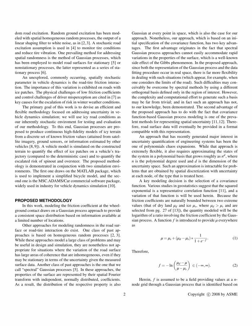
Figure 1. Gaussian processes are used to compute sampling character-istics on fine grid from deterministic data on sparse grid.

Samples at the n-node evaluation grid are obtained by draw-ing from a normal distribution with mean f∗ and covariance ma-trix COV(f∗):

f(x∗)∼ N(f∗,COV(f∗)) ∈Rn . (9)

For each sample, a cubic spline is used in conjunction with thegenerated data to produce friction coefficients outside the n-nodegrid. During the simulation, the spline is invoked to evaluate fat all the road-tire contact points at any time, as shown in Figure4. The equations of motion are formulated and solved by usingfriction coefficient input from the constructed spline. The vehi-cle positions and velocities are computed for each sample andaveraged; furthermore, variance is computed at each simulationtime step.

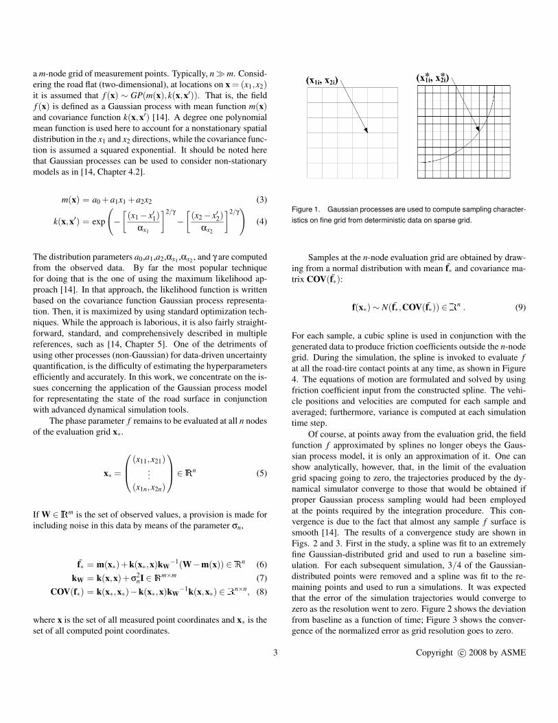
Of course, at points away from the evaluation grid, the fieldfunction f approximated by splines no longer obeys the Gaus-sian process model, it is only an approximation of it. One canshow analytically, however, that, in the limit of the evaluationgrid spacing going to zero, the trajectories produced by the dy-namical simulator converge to those that would be obtained ifproper Gaussian process sampling would had been employedat the points required by the integration procedure. This con-vergence is due to the fact that almost any sample f surface issmooth [14]. The results of a convergence study are shown inFigs. 2 and 3. First in the study, a spline was fit to an extremelyfine Gaussian-distributed grid and used to run a baseline sim-ulation. For each subsequent simulation, 3/4 of the Gaussian-distributed points were removed and a spline was fit to the re-maining points and used to run a simulations. It was expectedthat the error of the simulation trajectories would converge tozero as the resolution went to zero. Figure 2 shows the deviationfrom baseline as a function of time; Figure 3 shows the conver-gence of the normalized error as grid resolution goes to zero.


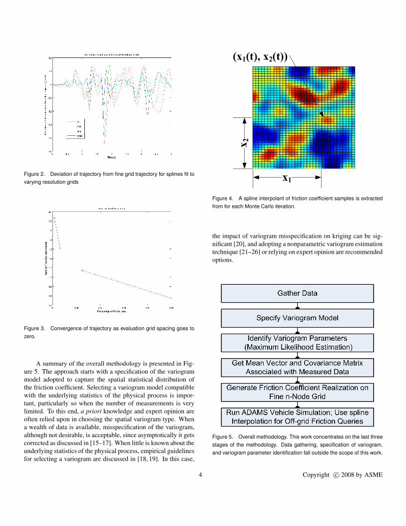
Figure 2. Deviation of trajectory from fine grid trajectory for splines fit tovarying resolution grids

Figure 3. Convergence of trajectory as evaluation grid spacing goes tozero.

A summary of the overall methodology is presented in Fig-ure 5. The approach starts with a specification of the variogrammodel adopted to capture the spatial statistical distribution ofthe friction coefficient. Selecting a variogram model compatiblewith the underlying statistics of the physical process is impor-tant, particularly so when the number of measurements is verylimited. To this end, a priori knowledge and expert opinion areoften relied upon in choosing the spatial variogram type. Whena wealth of data is available, misspecification of the variogram,although not desirable, is acceptable, since asymptotically it getscorrected as discussed in [15–17]. When little is known about theunderlying statistics of the physical process, empirical guidelinesfor selecting a variogram are discussed in [18, 19]. In this case,

Figure 4. A spline interpolant of friction coefficient samples is extractedfrom for each Monte Carlo iteration.

the impact of variogram misspecification on kriging can be sig-nificant [20], and adopting a nonparametric variogram estimationtechnique [21–26] or relying on expert opinion are recommendedoptions.

Figure 5. Overall methodology. This work concentrates on the last threestages of the methodology. Data gathering, specification of variogram,and variogram parameter identification fall outside the scope of this work.


MODELS CONSIDERED

The first model considered is a simple bicycle model imple-mented in MATLAB. An open-loop step steer angle is used tonegotiate a turn. A high-fidelity car model is used as well. Thevehicle is modeled in MSC.ADAMS/Car and is used to performa J-turn maneuver: drive straight up to a certain point, then ap-ply a ramp steer input to the steering wheel. These models arepresented in more detail in the following subsections.

Bicycle Model

The bicycle model, shown in Figure 6, has three degrees offreedom: longitudinal motion Vx, lateral motion Vy, and yaw Ωz.Three input functions determine the behavior of the model: steerangle δ f (t) and the front/rear wheel road adhesion coefficientsµ f and µr, respectively.

Figure 6. Bicycle model used in preliminary research of methodology[13].

After neglecting roll and asymetry and assuming that nothrust forces exist (that is, the vehicle coasts into the turn), thegoverning differential equations for vehicle velocities and posi-tions are

m(Vx−VyΩz) = −Fy f sinδ f

m(Vy +VxΩz) = Fyr +Fy f cosδ f (10)IzΩz = l1Fy f cosδ f − l2Fyr

X = Vx cosΘz−Vy sinΘz

Y = Vx sinΘz +Vy cosΘz (11)Θz = Ωz.

The geometric parameters for the bicycle were taken from[27]. The constitutive equations for the forces acting on the tiresare provided by [13].

Fy f =

µpW f2tanαc

tanα f α f ≤ αc

µpWf (1− tanαc2tanα f

) α f > αc(12)

Fyr =

µpWr

2tanαctanαr αr ≤ αc

µpWr(1− tanαc2tanαr

) αr > αc(13)

Wf and Wr are the front and back tire normal forces, respectively;α is the respective slip angle for each tire; µp is the respectivepeak road adhesion coefficient for each tire; and αc is the criticalslip angle.

Geometrically, the slip angles are related to the state vari-ables and the steer angle alone.

α f = δ f − arctanl1Ωz +Vy

Vx(14)

αr = arctanl2Ωz−Vy

Vx(15)

ADAMS Car ModelThe more sophisticated vehicle model is obtained through

MSC.ADAMS/Car, a full vehicle simulation package distributedby MSC.Software. The vehicle parameters used were taken di-rectly from the default MSC.ADAMS/Car library. The full ve-hicle model is the integration of several subsystems includinga rack-and-pinion type steering subsystem, an Ackerman armsuspension system, and a flexible chassis. Figure 7 shows thetopology of a vehicle with front and rear suspension, wheels, andsteering subsystems (the chassis is not shown).

The test rig is a special subsystem that conveys user inputsfor steering angle to the model. ADAMS/View variables called”Communicators” are used to communicate between the subsys-tems.


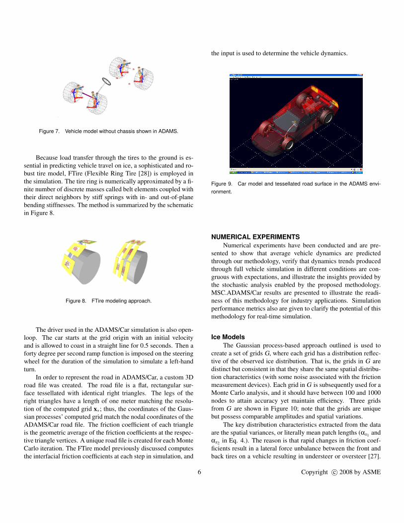
Figure 7. Vehicle model without chassis shown in ADAMS.

Because load transfer through the tires to the ground is es-sential in predicting vehicle travel on ice, a sophisticated and ro-bust tire model, FTire (Flexible Ring Tire [28]) is employed inthe simulation. The tire ring is numerically approximated by a fi-nite number of discrete masses called belt elements coupled withtheir direct neighbors by stiff springs with in- and out-of-planebending stiffnesses. The method is summarized by the schematicin Figure 8.

Figure 8. FTire modeling approach.

The driver used in the ADAMS/Car simulation is also open-loop. The car starts at the grid origin with an initial velocityand is allowed to coast in a straight line for 0.5 seconds. Then aforty degree per second ramp function is imposed on the steeringwheel for the duration of the simulation to simulate a left-handturn.

In order to represent the road in ADAMS/Car, a custom 3Droad file was created. The road file is a flat, rectangular sur-face tessellated with identical right triangles. The legs of theright triangles have a length of one meter matching the resolu-tion of the computed grid x∗; thus, the coordinates of the Gaus-sian processes’ computed grid match the nodal coordinates of theADAMS/Car road file. The friction coefficient of each triangleis the geometric average of the friction coefficients at the respec-tive triangle vertices. A unique road file is created for each MonteCarlo iteration. The FTire model previously discussed computesthe interfacial friction coefficients at each step in simulation, and

the input is used to determine the vehicle dynamics.

Figure 9. Car model and tessellated road surface in the ADAMS envi-ronment.

NUMERICAL EXPERIMENTSNumerical experiments have been conducted and are pre-

sented to show that average vehicle dynamics are predictedthrough our methodology, verify that dynamics trends producedthrough full vehicle simulation in different conditions are con-gruous with expectations, and illustrate the insights provided bythe stochastic analysis enabled by the proposed methodology.MSC.ADAMS/Car results are presented to illustrate the readi-ness of this methodology for industry applications. Simulationperformance metrics also are given to clarify the potential of thismethodology for real-time simulation.

Ice ModelsThe Gaussian process-based approach outlined is used to

create a set of grids G, where each grid has a distribution reflec-tive of the observed ice distribution. That is, the grids in G aredistinct but consistent in that they share the same spatial distribu-tion characteristics (with some noise associated with the frictionmeasurement devices). Each grid in G is subsequently used for aMonte Carlo analysis, and it should have between 100 and 1000nodes to attain accuracy yet maintain efficiency. Three gridsfrom G are shown in Figure 10; note that the grids are uniquebut possess comparable amplitudes and spatial variations.

The key distribution characteristics extracted from the dataare the spatial variances, or literally mean patch lengths (αx1 andαx2 in Eq. 4.). The reason is that rapid changes in friction coef-ficients result in a lateral force unbalance between the front andback tires on a vehicle resulting in understeer or oversteer [27].


Figure 10. Phase parameter grids created from the same set of ob-served data.

The grids shown in Figure 11 are from two different sets of ob-served data: the top plot from a mean patch length of one meterand the bottom plot from a mean patch length of three meters.These grids demonstrate the sensitivity of the methodology tospatial variance.

As indicated earlier, in order to account for the biextremalnature of the friction coefficient, a phase parameter f – the log-arithm of a ratio involving the friction coefficient – is used. TheGaussian process is exercised on the phase parameter distribu-tion, creating a phase parameter grid that is subsequently trans-formed to a friction coefficient grid. Figure 12 shows a realiza-tion of f on a grid and the corresponding realization of µ on thesame grid.

The grids used in the following simulations were producedfrom randomly generated data assuming the values of distribu-tion parameter from Eqs. 3 and 4: a0=a1=a2=0, γ=1, and σn=.15.Different parameters, αx1 and αx2 , were used in experimentation

Figure 11. Phase parameter grids created from data sets with meanpatch lengths one meter (top) and three meters (bottom).

and are stated for individual tests as mean patch lengths.

Bicycle SimulationThe bicycle dynamics were investigated in MATLAB, and

two simulation outcomes were monitored: yaw velocity, to gaugespin-out and instability, and global position, to gauge deviationfrom the desired path as a product of slip, oversteer, or under-steer. Simulations were first run with deterministic conditions,and Figures 13 and 14 show the friction input to each bicycle tiresand the yaw velocity output as functions of time, respectively.The greatest instabilities occur during rapid friction changes; thehigh yaw rates are reached when the front steering tire has moretraction than the rear tire (particularly between 13 and 14 secondsin simulation time).

Gaussian processes were implemented and simulations runfor several vehicle conditions including a variety of speed andsteer angles. Different data sets were used to represent road con-ditions. The simulation results shown in Figs. 15 and 16 are forhigh and low ice densities, respectively. Several interesting sim-ilarities exist between the two simulations and across the othersimulations conducted. First, the average response (dynamics)of the vehicle is far from the constant friction case; this disparityresults in deviation from the desired travel path and makes navi-gation more difficult. Second, as shown in Figure 17, the uncer-tainty in the response tends to increase in time or with distance


Figure 12. Transformation from the phase parameter grid (top) to thefriction coefficient grid (bottom).

traveled. This illustrates the danger of long turns if the driveris not vigilant at the wheel. As the driver progresses around theturn, the risk of instability increases. Third, the uncertainty of thevehicle dynamics is varying in space, as seen in Figure 17. Wehave noticed that deep local minima in the yaw uncertainty cor-respond to passing near a known data point as verified by com-paring the global position at these time iterations with the ob-served data coordinates. That is perhaps to be expected, thoughthe depth of some of those minima was surprising to us giventhat for dynamical systems the uncertainty tends to grow fairlysteadily in time. Whether higher certainty of a surface patch statecan be exploited in a control procedure is an interesting topic forfuture research.

An experiment was set up to validate the predictive capa-bility of the methodology. The original random set of frictioncoefficients was amended to introduce a strip of abrupt ice (lowfriction coefficients) approximately two seconds into the vehi-cle’s travel. The result of the simulation is shown in Figure 18;the constant friction simulation would have resulted in a yaw ve-locity of approximately 0.2 but it is not shown for the sake ofclarity. Clearly, the Gaussian process accounts for the ice strip

Figure 13. Deterministic simulation: friction coefficient input.

Figure 14. Deterministic simulation: resulting vehicle dynamics.

as nearly all Monte Carlo iterations diverge drastically from theconstant friction dynamics. The resulting average indicates thatthe driver will experience an uncomfortable change in yaw veloc-ity and should enter the turn at a lower speed. Incidentally, thedrop in yaw around 3.5 seconds was the result not of a manualice insertion but rather of a coincidental low friction coefficientgrouping generated randomly.

ADAMS Car SimulationTo demonstrate the propensity of our methodology for

industry applications, we introduced our ice model intoMSC.ADAMS/Car. The car model used considers several ve-hicle subsystems and intersystem interactions to produce high-


Figure 15. Bicycle simulation: one-meter mean patch length, one de-gree steer angle, 200 Monte Carlo iterations.

Figure 16. Bicycle simulation: three-meter mean patch length, one de-gree steer angle, 200 Monte Carlo iterations.

fidelity results as explained in the Models Considered section.The results shown in Figs. 19 and 20 are for the simulation ofa car executing a left turn on an icy road. The observed frictiondata, for the results shown, was generated randomly and thenmanipulated to introduce a strip of ice expectedly two secondsinto the vehicle’s travel. The Gaussian process results in Figure19 possess the same three characteristics discussed in the Bicyclemodel results: divergence from the constant friction case, prolif-eration of uncertainty with time, and alternating uncertainty de-pending on proximity to observed data coordinates. The paths oftravel shown in Figure 20 are one example of how our method-

Figure 17. Dynamical uncertainty as a function of time: one meter patchlength, one degree steer angle, 200 Monte Carlo iterations.

Figure 18. Gaussian process simulation with implanted ice strip: three-meter mean patch length, one degree steer angle, 200 Monte Carlo iter-ations.

ology could be an asset to visualization and communication inindustry. Moreover, the divergence from the desired turn is theresult of the strip of ice in the road and possibly other smallerpatches accumulated in the randomly generated data; quantify-ing the magnitude of this divergence is essential to driver safety.

DiagnosticsFor this methodology to be useful in an industry setting, it

has to produce results fast and reliably. To understand the run-time characteristics of the simulation processes, we monitor theduration of generating a realization x∗ for different simulationtimes (Figure 21), different evaluation grid (x∗) resolutions (Fig-ure 22), and different sample grid ((x) resolutions (Figure 23).


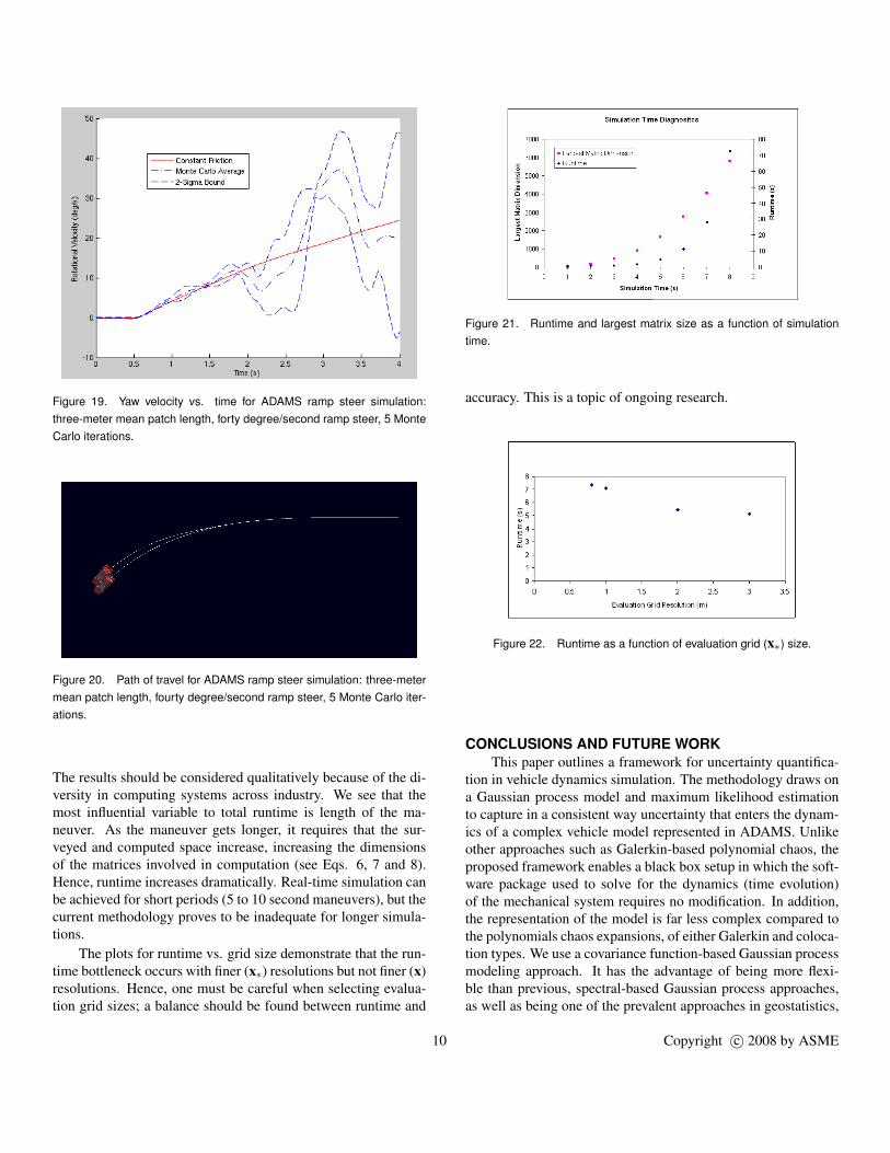
Figure 19. Yaw velocity vs. time for ADAMS ramp steer simulation:three-meter mean patch length, forty degree/second ramp steer, 5 MonteCarlo iterations.

Figure 20. Path of travel for ADAMS ramp steer simulation: three-metermean patch length, fourty degree/second ramp steer, 5 Monte Carlo iter-ations.

The results should be considered qualitatively because of the di-versity in computing systems across industry. We see that themost influential variable to total runtime is length of the ma-neuver. As the maneuver gets longer, it requires that the sur-veyed and computed space increase, increasing the dimensionsof the matrices involved in computation (see Eqs. 6, 7 and 8).Hence, runtime increases dramatically. Real-time simulation canbe achieved for short periods (5 to 10 second maneuvers), but thecurrent methodology proves to be inadequate for longer simula-tions.

The plots for runtime vs. grid size demonstrate that the run-time bottleneck occurs with finer (x∗) resolutions but not finer (x)resolutions. Hence, one must be careful when selecting evalua-tion grid sizes; a balance should be found between runtime and

Figure 21. Runtime and largest matrix size as a function of simulationtime.

accuracy. This is a topic of ongoing research.

Figure 22. Runtime as a function of evaluation grid (x∗) size.

CONCLUSIONS AND FUTURE WORKThis paper outlines a framework for uncertainty quantifica-

tion in vehicle dynamics simulation. The methodology draws ona Gaussian process model and maximum likelihood estimationto capture in a consistent way uncertainty that enters the dynam-ics of a complex vehicle model represented in ADAMS. Unlikeother approaches such as Galerkin-based polynomial chaos, theproposed framework enables a black box setup in which the soft-ware package used to solve for the dynamics (time evolution)of the mechanical system requires no modification. In addition,the representation of the model is far less complex compared tothe polynomials chaos expansions, of either Galerkin and coloca-tion types. We use a covariance function-based Gaussian processmodeling approach. It has the advantage of being more flexi-ble than previous, spectral-based Gaussian process approaches,as well as being one of the prevalent approaches in geostatistics,


Figure 23. Runtime as a function of sample grid (x) size.

making it likely that this approach will be easy to use in con-junction with emerging spatial database technology. Insofar assimulation, once the Gaussian process model over the road sur-face is obtained, the methodology relies on a Monte Carlo stepthat generates the information required to produce the vehicledynamics statistics of interest.

Several steps have not been discussed here but are being ad-dressed in ongoing projects. First, work is underway to extendthe Gaussian process-based uncertainty model to other classesof models, including nonstationary models. Since in kriging thechoice of weights is completely determined by the choice of thevariogram model, it is particularly important for handling spatialuncertainty (road-tire friction coefficients, road elevation) to lookat other models beyond Gaussian processes. Since a Gaussianprocess approach is guaranteed to work provided the amount ofmeasured data is large, other questions of interest are how to han-dle effectively large sets of measurements and how to use consis-tently and update periodically subsets of data to handle only sub-regions of interest. The latter would allow one to handle smallerregions of data that are surrounding the vehicle as it moves on aroad.

The methodology presented was illustrated for an applica-tion where the source of uncertainty is provided by the road/tirefriction coefficient. It remains to investigate how road profileuncertainty reflects in the overall vehicle dynamics. Such an un-dertaking critically depends on the quality of the tire models usedin the vehicle simulation. However, the FTire model relied on inthis work provides a level of fidelity for fully three-dimensionalsimulation that makes terrain-uncertainty investigation possibleand likely to be very insightful.

ACKNOWLEGMENTSDr. Bahram Fatemi and Dr. Reza Shadeghi are gratefully

acknowledged for facilitating the research support coming fromBritish Aerospace Engineering (BAE) and MSC.Software, re-spectively, that made possible the portion of this work carried

out in the Simulation Based Engineering Lab at the University ofWisconsin, Madison. Mihai Anitescu was supported by ContractNo. DE-AC02-06CH11357 of the U.S. Department of Energy.

REFERENCES[1] Robson, J., and Dobbs, C., 1975. “Stochastic road inputs

and vehicle response”. Vehicle System Dynamics, 5, pp. 1–3.

[2] Narayanan, S., 1990. “Stochastic optimal-control of non-stationary response of a single degree-of freedom vehiclemodel”. Journal of Sound and Vibration, 141, pp. 449–463.

[3] Hammond, J. K., and Harrison, R. F., 1984. Covarianceequivalent forms and evolutionary spectra for nonstation-ary random processes, Vol. 62. Springer Berlin/Heidelberg.

[4] Rustighi, E., and Elliot, J. S., 2007. “Stochastic road ex-citation and control feasibility in a 2d linear tyre model”.Journal of Sound and Vibration, 300, pp. 490–501.

[5] Lei, X., and Noda, N., 2002. “Analyses of dynamic re-sponse of vehicle and track coupling system with randomirregularity of track vertical profile”. Journal of Sound andVibration, 258, pp. 147–165.

[6] Karacay, T., Akturk, N., and Eroglu, M., 2004. “Non-stationary response of a vehicle obtained from a series ofstationary responses”. KSME International Journal, 18,pp. 1565–1571.

[7] Wallman, C., and Astrom, H., 2001. “Friction measurementmethods and the correlation between road friction and traf-fic safety. a literature review.”. VTI meddelande 911A.

[8] Holzmann, F., Bellino, M., Siegwart, R., and Bubb, H.,2006. “Predictive estimation of the road-tire friction coeffi-cient”. In Control Applications IEEE International Confer-ence.

[9] Rajamni, R., Piyabongkarn, D., Lew, J., and Grogg, J.,2006. “Algorithms for real-time estimation of individualwheel tire-road friction coefficients”. In American ControlConference.

[10] MSC.Software, 2005. ADAMS User Manual. Availableonline at http://www.mscsoftware.com.

[11] Chiles, J. P., and Delfiner, P., 1999. Geostatistics: modelingspatial uncertainty. Wiley, New York.

[12] Stein, M., 1999. Interpolation of Spatial Data: Some The-ory for Kriging. Springer.

[13] Wong, J., 2001. Theory of Ground Vehicles. John Wiley &Sons, Inc.

[14] Rasmussen, C., and Williams, C., 2006. Gaussian Pro-cesses for Machine Learning. MIT Press.

[15] Stein, M., 1988. “Asymptotically efficient prediction ofa random field with a misspecified covariance function”.Ann. Stat, 16, pp. 55–63.

[16] Stein, M., 1990. “Uniform asymptotic optimality of lin-


ear predictions of a random field using an incorrect second-order structure”. Ann. Statist, 18(2), pp. 850–872.

[17] Stein, M., and Handcock, M., 1989. “Some asymptoticproperties of kriging when the covariance function is mis-specified”. Mathematical Geology, 21(2), pp. 171–190.

[18] Journel, A., and Huijbregts, C., 1978. “Mining Geostatis-tic”. Academic, San Diego.

[19] Clark, I., 1979. Practical geostatistics. Applied SciencePublishers, London.

[20] Gorsich, D., and Genton, M., 2000. “Variogram Model Se-lection via Nonparametric Derivative Estimation”. Mathe-matical Geology, 32(3), pp. 249–270.

[21] Shapiro, A., and Botha, J., 1991. “Variogram fitting witha general class of conditionally nonnegative definite func-tions.”. Computational Statistics & Data Analysis, 11(1),pp. 87–96.

[22] Lele, S., 1995. “Inner product matrices, kriging, and non-parametric estimation of variogram”. Mathematical Geol-ogy, 27(5), pp. 673–692.

[23] Cherry, S., 1996. “An evaluation of a non-parametricmethod of estimating semi-variograms of isotropic spatialprocesses”. Journal of Applied Statistics, 23(4), pp. 435–449.

[24] CHERRY, S., 1997. “NON-PARAMETRIC ESTIMATIONOF THE SILL IN GEOSTATISTICS”. Environmetrics,8(1), pp. 13–27.

[25] Ecker, M., and Gelfand, A., 1997. “Bayesian variogrammodeling for an isotropic spatial process”. Journal ofAgricultural, Biological and Environmental Statistics, 2(4),pp. 347–369.

[26] Genton, M., and Gorsich, D., 2002. “Nonparametric var-iogram and covariogram estimation with Fourier–Besselmatrices”. Computational Statistics and Data Analysis,41(1), pp. 47–57.

[27] Cossalter, V., 2002. Motorcycle Dynamics. Race DynamicsInc.

[28] Gipser, M., 2005. “Ftire: a physically based application-oriented tyre model for use with detailed mbs and finite-element suspension models”. Vehcile System Dynamics, 43(supplment), pp. 76–91.

The submitted manuscript has been created in part byUChicago Argonne, LLC, operator of Argonne National Lab-oratory (”Argonne”). Argonne, a U.S. Department of EnergyOffice of Science laboratory, is operated under Contract No.DE-AC02-06CH11357. The U.S. Government retains for it-self, and others acting on its behalf, a paid-up nonexclusive,irrevocable worldwide license in said article to reproduce, pre-pare derivative works, distribute copies to the public, and per-form publicly and display publicly, by or on behalf of the Gov-ernment.


a gaussian process-based approach for … · ondone isthe msc.adams/car commercial software...

Documents