a full multigrid implementation on staggered adaptive
TRANSCRIPT

you don’t see
Technische Universitat Munchen
Computational Science and Engineering
(Int. Master’s Program)
Master’s Thesis
A Full Multigrid Implementation on StaggeredAdaptive Cartesian Grids for the PressurePoisson Equation in Computational Fluid
Dynamics
Michael Lieb

Contents
1 Introduction 1
2 Poisson Equation in Fluid Dynamics 32.1 Partial Differential Equations . . . . . . . . . . . . . . . . . . . . . . 32.2 The Poisson Equation in Fluid Dynamics . . . . . . . . . . . . . . . . 32.3 Grids . . . . . . . . . . . . . . . . . . . . . . . . . . . . . . . . . . . . 42.4 Grids for Fluid Dynamics . . . . . . . . . . . . . . . . . . . . . . . . 4
3 Fundamentals 73.1 Spacetrees . . . . . . . . . . . . . . . . . . . . . . . . . . . . . . . . . 73.2 Space-Filling Curves . . . . . . . . . . . . . . . . . . . . . . . . . . . 103.3 Traversal of Grids Using Peano Curves . . . . . . . . . . . . . . . . . 113.4 Notations . . . . . . . . . . . . . . . . . . . . . . . . . . . . . . . . . 11
3.4.1 Systems of Linear Equations . . . . . . . . . . . . . . . . . . . 123.4.2 Sub- and Superscripts . . . . . . . . . . . . . . . . . . . . . . 12
3.5 Iterative Schemes . . . . . . . . . . . . . . . . . . . . . . . . . . . . . 123.6 Residual Based Notation . . . . . . . . . . . . . . . . . . . . . . . . . 133.7 Boundary Conditions . . . . . . . . . . . . . . . . . . . . . . . . . . . 14
3.7.1 Dirichlet Boundary Conditions . . . . . . . . . . . . . . . . . . 143.7.2 Neumann Boundary Conditions . . . . . . . . . . . . . . . . . 14
4 Multigrid Algorithms 154.1 Multigrid Notations . . . . . . . . . . . . . . . . . . . . . . . . . . . . 154.2 Galerkin Approximation . . . . . . . . . . . . . . . . . . . . . . . . . 174.3 Correction Storage Scheme . . . . . . . . . . . . . . . . . . . . . . . . 174.4 Full Approximation Storage Scheme . . . . . . . . . . . . . . . . . . . 184.5 Hierarchical Transformation Scheme . . . . . . . . . . . . . . . . . . . 20
5 Geometry Discretization 25
6 HT-MG on Staggered Adaptive Cartesian Grids 276.1 Information Transfer Using Bilinear Interpolation . . . . . . . . . . . 276.2 Gauss-Seidel on a Cell Based Grid . . . . . . . . . . . . . . . . . . . . 296.3 Boundary Conditions on Staggered Grids . . . . . . . . . . . . . . . . 32
6.3.1 Dirichlet Boundary Conditions . . . . . . . . . . . . . . . . . . 326.3.2 Neumann Boundary Conditions . . . . . . . . . . . . . . . . . 336.3.3 Modification of the Diagonal Elements . . . . . . . . . . . . . 34
I

Contents
6.4 Coarsening of a Staggered Grid . . . . . . . . . . . . . . . . . . . . . 346.5 Calculation of the Hierarchical Surplus . . . . . . . . . . . . . . . . . 366.6 Computing the Hierarchical Residual . . . . . . . . . . . . . . . . . . 386.7 Restriction of the Hierarchical Residual . . . . . . . . . . . . . . . . . 396.8 Inverse Hierarchical Transformation . . . . . . . . . . . . . . . . . . . 40
7 Challenges and Technical Solutions 437.1 The Peano Framework . . . . . . . . . . . . . . . . . . . . . . . . . . 43
7.1.1 Technical Representation of Information . . . . . . . . . . . . 437.1.2 Grid Initialization . . . . . . . . . . . . . . . . . . . . . . . . . 447.1.3 Grid Operations for Solvers . . . . . . . . . . . . . . . . . . . 45
7.2 HT-MG Scheme in Peano . . . . . . . . . . . . . . . . . . . . . . . . 467.3 Stencil Implementations . . . . . . . . . . . . . . . . . . . . . . . . . 50
7.3.1 Skew Stencil . . . . . . . . . . . . . . . . . . . . . . . . . . . . 507.3.2 Standard Stencil . . . . . . . . . . . . . . . . . . . . . . . . . 51
8 Numerical Experiments 538.1 Test Scenarios . . . . . . . . . . . . . . . . . . . . . . . . . . . . . . . 53
8.1.1 Sinus . . . . . . . . . . . . . . . . . . . . . . . . . . . . . . . 538.1.2 Increased Activity . . . . . . . . . . . . . . . . . . . . . . . . . 53
8.2 Gauss-Seidel . . . . . . . . . . . . . . . . . . . . . . . . . . . . . . . . 548.2.1 Peano Curve Based Traversal . . . . . . . . . . . . . . . . . . 548.2.2 Relaxed Gauss-Seidel . . . . . . . . . . . . . . . . . . . . . . . 56
8.3 HT-MG Convergence Analysis . . . . . . . . . . . . . . . . . . . . . . 56
9 Conclusions 61
A HT-MG operations 63A.1 Neighbor Reconstruction of Inner Cells . . . . . . . . . . . . . . . . . 63A.2 Interpolation Values of Hierarchical Surplus . . . . . . . . . . . . . . 64
II
Zusammenfassung
Mehrgitteralgorithmen gehoren zu den effizientesten Algorithmen zur Losung lin-earer Gleichungsysteme, die aus der Diskretisierung partieller Differentialgleichun-gen (PDEs) resultieren. Eines der bekanntesten Beispiele sind wohl die Poisson-Gleichungen, welche zahlreiche physikalische Problemstellungen beschreiben. Indieser Arbeit untersuchen wir einen geometrischen Mehrgitterloser zur Losung Poisson-artiger Gleichungen, welche aus den Massenerhaltungsgesetzen der Fluiddynamikhervorgehen.
Die Simulation von Problemen der Fluiddynamik geht einher mit hohen An-forderungen an Rechenleistung und Speicherkapazitat. Daher ist es wichtig, einenhochperformanten Code mit gleichzeitig niedrigem Speicherbedarf zur Verfugung zuhaben. Dabei sollte gewahrleistet sein, dass numerische Funktionalitat - wie etwadynamische Adaptivitat, Mehrgitterdiskretisierung und Parallelisierbarkeit - weit-erhin erhalten bleibt. Diese Anforderungen motivierten die Implementierung einerEntwicklungsumgebung fur die Losung partieller Differentialgleichungen auf adap-tiven kartesischen Gittern. Diese Entwicklungsumgebung wird Peano genannt.
Zwei zentrale Eigenschaften fuhren zu den niedrigen Speicheranforderungen vonPeano. Das ware zum einen der Verzicht auf globale Assemblierungsmatrizen, zumanderen das strikt elementweise Operieren. Hierfur werden die Losungsfunktioneneines Losers in eine hierarchische Gittertraversierung eingebunden. Es war vor Be-ginn dieser Arbeit bereits bekannt wie additive und multiplikative geometrischeMehrgitteralgorithmen in einen elementweise operierenden Algorithmus einzubindensind, allerdings nur unter der Einschrankung, dass die Positionen der Unbekanntender PDE an den Ecken des Gitters liegen.
Die Poisson Gleichung innerhalb des in Peano implementierten Stromungsloserserfordert jedoch Unbekannte, welche auf den Zellmittelpunkten platziert sind. Beiderartigen Gittern mussen dann samtliche Zugriffsmuster, wie die Operatorauswer-tungsordnung und die Operatormatrizen an die elementweise Traversierung angepasstwerden.
Solche Formalismen existieren bereits fur additiv geometrische Mehrgitterloserauf regularen kartesischen Gittern. Mit dieser Arbeit werden die Konzepte zueinem multiplikativen Mehrgitter hin ausgeweitet. Daruber hinaus wird die Imple-mentierung von Neumann-Randbehandlungen eingefuhrt, wo bisher nur Dirichlet-Randbehandlungen verfugbar waren, die Speichereffizienz erhoht und drei verschiedeneOperatoren implementiert. Der Algorithmus wird als ”Full Approximation Scheme”implementiert. Somit ist die Approximation einer Losung zeitgleich auf verschiede-nen Gittern prasent. Diese Eigenschaft vereinfacht die Verwendung adaptiver Gittererheblich und ist somit von hohem Wert. Das Verhalten der implementierten Loser
III

Contents
wird abschließend in einigen einfachen Poisson-Testszenarien untersucht.
IV
Abstract
Multigrid methods are among the most efficient algorithms for solving linear equa-tion systems arising from partial differential equations (PDEs). The most populardifferential equations are perhaps the Poisson equations. They are part of manyphysical problems. In this thesis, we study a geometric multigrid solver for thePoisson-like equation induced by the mass conservation in fluid dynamics.
Simulation codes in fluid dynamics come along with high computational demandsand large data sets. Thus, it is important to have a high performance code with lowmemory requirements that still offers all the features today’s numerics require for.For example: Dynamic adaptivity, multilevel discretization and parallel scalabil-ity. Among others, these requirements motivated the development of a PDE solverframework working on adaptive Cartesian grids. The framework is called Peano.
There are two key ingredients, leading to the low memory requirements of Peano.The first is that it works without global system matrices, second it works in astrictly element-wise way. This means, the solvers’ computations are embedded intothe hierarchical grid traversal. It is well known, how to implement additive andmultiplicative geometric multigrid algorithms in an element-wise algorithm, if thespatial positions of the PDE’s unknowns are aligned with the grid. The unknownsthen are located at the vertices of the grid.
The Poisson equation here requires for unknowns that are placed on the grid’scells, i.e. the grid belonging to the equation is staggered compared to the computa-tional grid. For such a grid, the whole data access scheme, the operator evaluationorder and the operator matrices of the multigrid algorithm have to be re-formalizedto make it fit to the element-wise traversal.
Such a formalism and such an algorithm for an additive geometric multigrid onregular Cartesian grids stemming from Peano exist for several years. In this thesis,we extend its idea to a multiplicative multigrid scheme. Furthermore, we discussthe implementation of Neumann boundary conditions instead of solely Dirichletboundary conditions, we reduce the code’s memory consumption further, we examinethree different operators (stencils), and we make the algorithm work with a fullapproximation storage scheme, such that the solution’s approximation is representedon different levels simultaneously. The latter ingredient simplifies the handling ofadaptive Cartesian grids and, thus, is of great value. The code’s behavior is studiedfor several simple Poisson problems.
V

Contents
VI

Acknowledgement
At this place I would like to express my gratitude to those who gave me the pos-sibility to complete this thesis. Special thanks to the executive president of TESISDYNAware, Dr. Cornelius Chucholowski, for giving me the opportunity to workand to participate in this Master’s program in parallel. Furthermore, it is a pleasureto thank all the people of the Chair of Scientific Computing for the friendly andsupportive environment. I am deeply indebted to my supervisor Tobias Weinzierl.His stimulating suggestions and encouragement helped me in all the time. Finally,I want to thank my examiners Prof. Hans-Joachim Bungartz and Prof. ThomasHuckle for their efforts to examine this work.
VII

Contents
VIII
1 Introduction
The following thesis has been developed within the fluid dynamics group in Com-puter Science at the TU-Munchen. The idea for it throughout after my participationin the CFD-Lab in WS07/08. This course gives, amongst others, an introductioninto linear equation system solvers.
The CFD-solvers implemented in the lab-course work with explicit time discretiza-tion. This principles are applied by research groups at the chair as well. The explicittime discretization leads to a sequence of Poisson equations. Thus, the performanceof CFD-solver stands or falls by performance of Poisson equation solvers. Theperformance is two-folded. It has to converge fast and exploit today’s hardwarecapablilities.
Multigrid algorithms come along with almost linear solution complexity for ellip-tic problems and are thus, a feasible solution. A research group at the chair hasdeveloped the Peano framework. It provides Peano curve based spacetree traver-sals. These are well-suited for the implementation of multigrid algorithms. Today’sapproaches developed in this framework are fast, cache-efficient, and make use ofdynamical grid refinement. However all are based on a nodal representation of theunknowns, i.e. all degrees of freedom are assigned to vertices. The solvers avoidthe formulation of global system matrices. Instead, element-wise update schemesare used. To fully make use of these concepts in CFD-solvers an implementation onstaggered grids is needed, i.e. the degrees of freedom are assigned to cells. Of cause,the solution must retain the good properties of nodal based implementations.
The principles of such an approach were already sketched in [16]. However, thereare many open points left. In this thesis, we realize the ideas discussed and extend itto a multiplicative multigrid scheme. Furthermore, we discuss the implementationof Neumann boundary conditions instead of solely Dirichlet boundary conditions.Introducing a new scheme for the information transfer among cells we reduce thecode’s memory consumption further, examine three different operators (stencils),and make the algorithm work with a full approximation storage scheme. Hence,the solution’s approximation is represented on different levels simultaneously. Thelast point prepares the handling of adaptive Cartesian grids. The code’s behavior isstudied for several simple Poisson problems.
1

1 Introduction
2

2 Poisson Equation in FluidDynamics
2.1 Partial Differential Equations
In Rd for d > 1 a partial differential equation (PDE) is defined on a domain Ω ⊂ Rd.A PDE contains the partial derivatives of an exact solution. In this thesis, we willdevelop a multigrid algorithm for the solution of elliptic boundary value problems.
A well-known example of an elliptic PDE is the Poisson equation
−4u(x) = f(x), x = (x0, . . . , xd−1) ∈ Ω. (2.1)
The equation 2.1 allows an infinite number of solutions. In order to get to a uniquesolution u, one has to define appropriate conditions on ∂Ω. Two ways to definethese conditions are presented in chapter 3.7. Depending on these conditions, thePoisson equation describes a number of physical phenomena, as e.g.
• the electrostatical potential,
• the gravitation potential,
• the pressure p = dFdA
as force per area.
2.2 The Poisson Equation in Fluid Dynamics
The mathematical model of non-stationary incompressible viscous fluids are theNavier-Stokes equations1:
∂tu+ (u∇)u− 1
Re4u+∇p = 0 u : Ω 7→ Rd. (2.2)
div u = 0 p : Ω 7→ R. (2.3)
The first term of these equations is called the momentum equation and describesthe behavior of a fluid in time. The terms are described as follows [16]:
• ∇p describes, in which direction fluid is pushed to reach a lower pressure area.
1The Equations 2.2 and 2.3 represent a dimensionless formulation of the Navier-Stokes equationsas they are formulated in [8].
3
2 Poisson Equation in Fluid Dynamics
• 1Re4u is called the diffusion term and describes how quickly variations in
velocity are damped-out, i.e. it describes the friction. The damping is scaledby the Reynolds number Re, describing the viscosity of the fluid.
• (∇u)u is called the advection term. It describes in what direction fluid isdragged by the surrounding fluid.
The second term is called the continuity equation. If we discretize the momentumequation with an explicit method and insert the resulting formula into the continuityequation for all time steps, this leads to a sequence of Poisson equations for thepressure. We concentrate on this pressure Poisson equation. A further discussion ofthe equations is omitted here, but detailed descriptions can be found in [11, 16, 17].
2.3 Grids
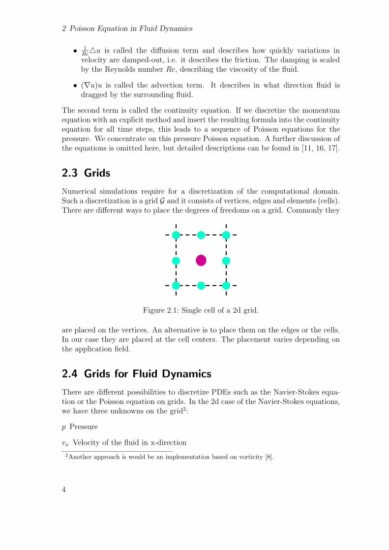
Numerical simulations require for a discretization of the computational domain.Such a discretization is a grid G and it consists of vertices, edges and elements (cells).There are different ways to place the degrees of freedoms on a grid. Commonly they
Figure 2.1: Single cell of a 2d grid.
are placed on the vertices. An alternative is to place them on the edges or the cells.In our case they are placed at the cell centers. The placement varies depending onthe application field.
2.4 Grids for Fluid Dynamics
There are different possibilities to discretize PDEs such as the Navier-Stokes equa-tion or the Poisson equation on grids. In the 2d case of the Navier-Stokes equations,we have three unknowns on the grid2:
p Pressure
vx Velocity of the fluid in x-direction
2Another approach is would be an implementation based on vorticity [8].
4

2.4 Grids for Fluid Dynamics
vy Velocity of the fluid in y-direction
The most simple approach is to place all information at one point in the grid. Suchgrids are called collocated grids. A small outcut of a collocated grid is depicted inFigure 2.2(a). A separation of the pressure and velocities but storing the velocities
(a) Collocated Grid (b) Partially Staggered Grid (c) (Fully) Staggered Grid
Figure 2.2: Grid types depending on the data locality.
at one point leads us to a so-called Partially Staggered Grid (Figure 2.2(b)). AFully Staggered Grid is a grid, where the pressure is placed in the cell center andthe velocities are placed separately on the edges of the cell. A sketch of a FullyStaggered Grid can be seen in Figure 2.2(b). Collocated grids lead to a number ofstability problems for our pressure Poisson equation. We thus concentrate on thecase where the unknown (pressure) is placed at the center of the cell.
5

2 Poisson Equation in Fluid Dynamics
6

3 Fundamentals
3.1 Spacetrees
If we want to compute the solution for a PDE numerically, we have to discretize thecomputational domain. We write Ω → Ωh. The discretization of a domain affectsthe quality of the numerical solution due to the discretization error. Usually, wereduce this discretization error going to finer grids [12]. If the discretization stepsize h of a regular Cartesian grid is reduced by a factor i, the number of unknownsn is increased depending on the dimension of the problem [13]:
n(h) 7→ n(h)di. (3.1)
The higher the number of unknowns n the more computational effort is needed to
(a) Domain Ω (b) Domain Ω embed-ded in the root cell c0 ∈G.
(c) The grid depictedrepresents the first regu-lar refinement level afterthe root level depictedin Figure 3.1(c).
(d) Domain Ω on aadaptively refined tri-partitioned grid. Thedepth of the grid isdepth(G) = 4.
Figure 3.1: Discretization of a continuous domain Ω on Cartesian grids.
solve the resulting equation system. In many cases, a finer grid is not needed allover the domain Ωh. This is where adaptive grids are used. Here, not the entiregrid has to be refined, but only certain regions where the discretization error harmsthe numerical solution. This could be for instance the boundary of the embeddeddomain Ω, as depicted in Figure 3.1(d). There are two classes of adaptive grids [10]:
• Adaptive structured grids, such as adaptive Cartesian grids, and
• unstructured grids, such as triangulations with triangles.
7
3 Fundamentals
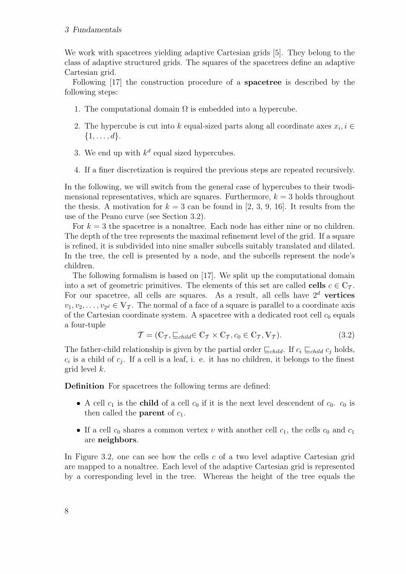
We work with spacetrees yielding adaptive Cartesian grids [5]. They belong to theclass of adaptive structured grids. The squares of the spacetrees define an adaptiveCartesian grid.
Following [17] the construction procedure of a spacetree is described by thefollowing steps:
1. The computational domain Ω is embedded into a hypercube.
2. The hypercube is cut into k equal-sized parts along all coordinate axes xi, i ∈1, . . . , d.
3. We end up with kd equal sized hypercubes.
4. If a finer discretization is required the previous steps are repeated recursively.
In the following, we will switch from the general case of hypercubes to their twodi-mensional representatives, which are squares. Furthermore, k = 3 holds throughoutthe thesis. A motivation for k = 3 can be found in [2, 3, 9, 16]. It results from theuse of the Peano curve (see Section 3.2).
For k = 3 the spacetree is a nonaltree. Each node has either nine or no children.The depth of the tree represents the maximal refinement level of the grid. If a squareis refined, it is subdivided into nine smaller subcells suitably translated and dilated.In the tree, the cell is presented by a node, and the subcells represent the node’schildren.
The following formalism is based on [17]. We split up the computational domaininto a set of geometric primitives. The elements of this set are called cells c ∈ CT .For our spacetree, all cells are squares. As a result, all cells have 2d verticesv1, v2, . . . , v2d ∈ VT . The normal of a face of a square is parallel to a coordinate axisof the Cartesian coordinate system. A spacetree with a dedicated root cell c0 equalsa four-tuple
T = (CT ,vchild∈ CT × CT , c0 ∈ CT ,VT ). (3.2)
The father-child relationship is given by the partial order vchild. If ci vchild cj holds,ci is a child of cj. If a cell is a leaf, i. e. it has no children, it belongs to the finestgrid level k.
Definition For spacetrees the following terms are defined:
• A cell c1 is the child of a cell c0 if it is the next level descendent of c0. c0 isthen called the parent of c1.
• If a cell c0 shares a common vertex v with another cell c1, the cells c0 and c1
are neighbors.
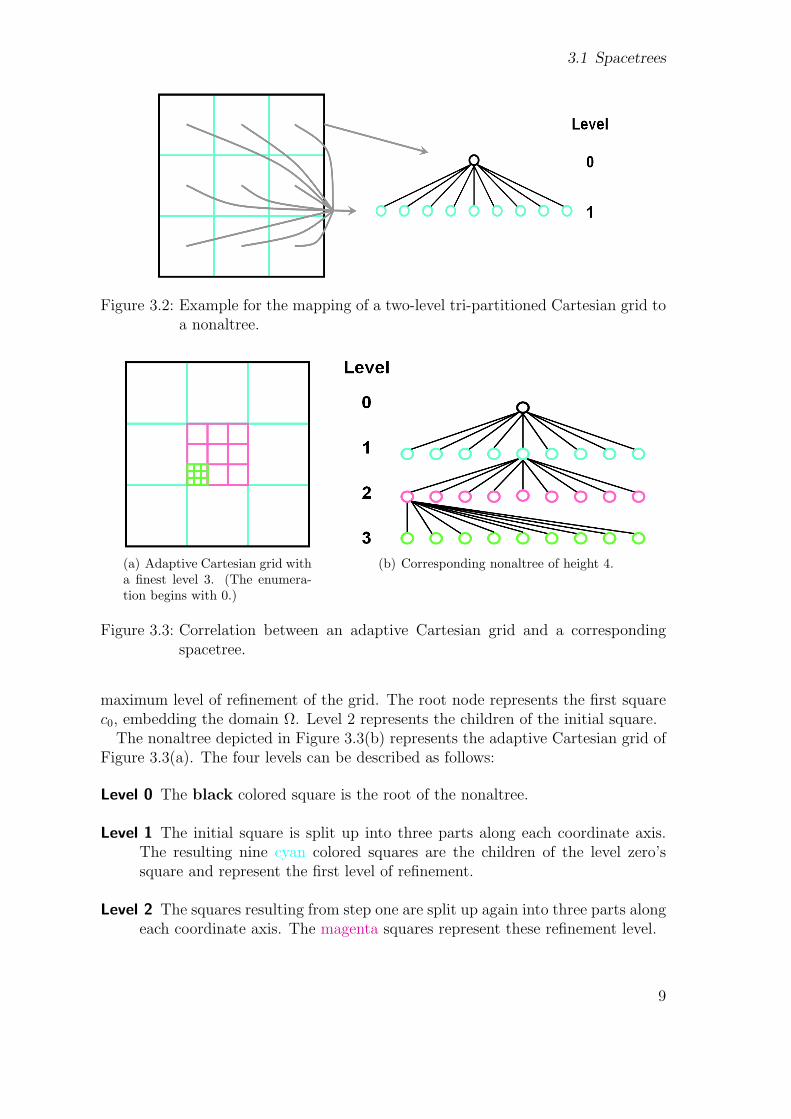
In Figure 3.2, one can see how the cells c of a two level adaptive Cartesian gridare mapped to a nonaltree. Each level of the adaptive Cartesian grid is representedby a corresponding level in the tree. Whereas the height of the tree equals the
8
3.1 Spacetrees
Figure 3.2: Example for the mapping of a two-level tri-partitioned Cartesian grid toa nonaltree.
(a) Adaptive Cartesian grid witha finest level 3. (The enumera-tion begins with 0.)
(b) Corresponding nonaltree of height 4.
Figure 3.3: Correlation between an adaptive Cartesian grid and a correspondingspacetree.
maximum level of refinement of the grid. The root node represents the first squarec0, embedding the domain Ω. Level 2 represents the children of the initial square.
The nonaltree depicted in Figure 3.3(b) represents the adaptive Cartesian grid ofFigure 3.3(a). The four levels can be described as follows:
Level 0 The black colored square is the root of the nonaltree.
Level 1 The initial square is split up into three parts along each coordinate axis.The resulting nine cyan colored squares are the children of the level zero’ssquare and represent the first level of refinement.
Level 2 The squares resulting from step one are split up again into three parts alongeach coordinate axis. The magenta squares represent these refinement level.
9

3 Fundamentals
Level 3 The green cells represent a further refinement according to the proceduredescribed before.
If a grid is organized equivalent to a tree data structure, the classical tree operations,algorithms and tree theory can be applied. Besides this, mapping grids to trees hasfurther advantages. Some of them are [3, 17]:
1. There is either a fixed number of children or none. Hence only one bit pernode is required to store the refinement information.
2. A mesh can easily be made dynamical adaptive.
3. A space or domain decomposition fits directly to the grids.
3.2 Space-Filling Curves
In 1878, Georg Cantor showed that the interval [0,1] can surjectively be mapped tothe square [0, 1]2 or the cube [0, 1]3. This is the fundamental mathematical insight,which goes hand in hand with the discovery of space filling curves [15].
Giuseppe Peano described the first space filling curve, which is nowadays knownas the Peano curve [15]. It’s construction can be described by the following threesteps:
1. Divide a quadratic domain in nine squares of the same size.
2. Connect the nine squares along a z-curve like in Figure 3.4(a).
3. Repeat the procedure recursively for each square.
These construction steps are depicted in Figures 3.4(a) to 3.4(c). A further descrip-
(a) Peano symbol (firstorder curve).
(b) The 2nd construc-tion step.
(c) 2nd order Peanocurve.
Figure 3.4: Development of a Peano Curve.
tion of the arithmetics and the definition can be found in [15].
10

3.3 Traversal of Grids Using Peano Curves
3.3 Traversal of Grids Using Peano Curves
In section 3.1, adaptive Cartesian grids are mapped to trees. If a numerical problemon such a grid is to be solved or the data of the grid are to be visualized, grid traversalalgorithms are needed. In this thesis, a cell-wise traversal1 is used [3, 9, 15, 17].
A tree based on the Peano curve in 2d is a nonaltree. It is an obvious idea tocombine a depth-first-search (DFS) with the cell order introduced by the Peanocurve. The result is a tree traversal for adaptive nonaltrees. The traversal of thefirst child level is illustrated in Figures 3.5(b) to 3.5(d). The enumeration of thecells indicates the traversal order.
(a) Whole grid. (b) Level 0. (c) Level 1. (d) Level 2.
Figure 3.5: An adaptive Cartesian grid with a cell enumeration based upon a Peanotraversal.
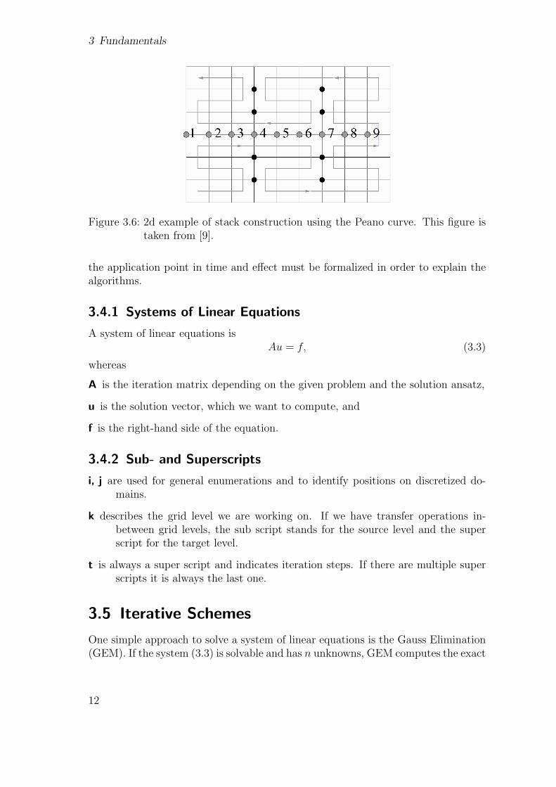
In Figure 3.6, one can see that the vertices on the middle line (marked by numbers1 to 9) are processed in ascending order in the lower part of the domain. Ascendingrefers to the vertex numbers. In the upper part of the domain the same elements areprocessed in descending order. For the Peano curve and regular grids, this linearforward and backward processing of the middle line can be shown for arbitrarilyfine grids, as well. In [9], a sophisticated data management concept based solely onstacks is introduced. Although this stack concept and the space-filling curves areimportant principles for the Peano framework, they are not that important for thisthesis as they do not affect the algorithms’ semantics. Yet, the order of the cellsdoes influence the numerical results, as we apply a Gauss-Seidel during the griditerations. In this iterative solver, the cell access sequence determines the updateorder of the unknowns. Different update orders result in quantitatively differentnumerical results.
3.4 Notations
The algorithms presented in this thesis require for some formalism, as there is a hugeset of different variables and operators with different representations. Furthermore,
1Cell-wise traversal and element-wise traversal are synonyms.
11
3 Fundamentals
Figure 3.6: 2d example of stack construction using the Peano curve. This figure istaken from [9].
the application point in time and effect must be formalized in order to explain thealgorithms.
3.4.1 Systems of Linear Equations
A system of linear equations isAu = f, (3.3)
whereas
A is the iteration matrix depending on the given problem and the solution ansatz,
u is the solution vector, which we want to compute, and
f is the right-hand side of the equation.
3.4.2 Sub- and Superscripts
i, j are used for general enumerations and to identify positions on discretized do-mains.
k describes the grid level we are working on. If we have transfer operations in-between grid levels, the sub script stands for the source level and the superscript for the target level.
t is always a super script and indicates iteration steps. If there are multiple superscripts it is always the last one.
3.5 Iterative Schemes
One simple approach to solve a system of linear equations is the Gauss Elimination(GEM). If the system (3.3) is solvable and has n unknowns, GEM computes the exact
12

3.6 Residual Based Notation
solution after O(n3) operations. Many problems in scientific computing today havelarge numbers of unknowns. At the same time, one can usually accept a solution, ifa certain level of accuracy ε is achieved. The reason is, that there are many othererrors like discretization or measurement errors which influence the linear equationsystem. There is no reason to solve such an inaccurate system exactly.
This is where iterative methods are applied. Such schemes work iteratively, i. e.at each iteration step t the error e is reduced. The goal of such methods is to performa fixed point iteration yielding a sequence of vectors ut, t ≥ 0 in R, converging tothe exact solution u. This means that
limt→∞
ut = u. (3.4)
However, the iteration is usually stopped, if a certain level of accuracy
‖ut − u‖ < ε (3.5)
is achieved. There are many ways to define ε and a well-suited vector norm ‖ · ‖. Adiscussion is beyond the scope of this thesis.
Many iterative schemes can be constructed based on an additive splitting of
A = Al − Au, (3.6)
which leads us then to the following abstract iteration scheme:
ut+1 = A−1l (Auu
t + f), t ≥ 0 (3.7)
To keep the effort as small as possible Al should be easily invertible. Depending onthe choice of Al, we get the following well-known methods:
Jacobi Al = diag(A), whereas diag extracts the diagonal entries of A.
Gauss-Seidel Al = U(A), whereas U is the upper diagonal matrix.
If we scale the Jacobi or Gauss-Seidel with a factor ω and add the trivial iteration(1 − ω)u(t+1) = (1 − ω)ut, we end up with damped Jacobi (ω ∈]0, 1]) or a relaxedGauss-Seidel (ω ∈]0, 2]).
3.6 Residual Based Notation
Let et be the error of a approximated solution of a system of linear equations intime step t. Then the residual is defined as follows [16]:
b = A(ut + et) = Aut + Aet,
rt = Aet = f − Aut.
Using this definition, we can reformulate the iteration schemes:
ut+1 = A−1l (Aru
t + f)
= A−1l (−Aut + f + Alu
t)
= ut + A−1l rt. (3.8)
13

3 Fundamentals
The damped Jacobi and the relaxed Gauss-Seidel correspond to
ut+1 = ut + ωA−1l rt+1. (3.9)
3.7 Boundary Conditions
The Poisson equation is an elliptic partial differential equation. To make ellipticPDEs solvable, one has to specify suitable conditions on the boundary ∂Ω of thedomain Ω ⊂ Rn. Within this thesis, two types of boundary conditions are used.
3.7.1 Dirichlet Boundary Conditions
Let u : Ω 7→ R be an elliptic differential equation with Dirichlet boundary conditions,i.e. the value of the solution on ∂Ω is prescribed:
−∆u = f ∀x ∈ Ω,
u|∂Ω = g.
Depending on the variable g we distinguish between
homogeneous g = 0 and
inhomogeneous g 6= 0
boundary conditions. If a value is a Dirichlet value, it is set before the system issolved and remains unchanged during the calculations.
3.7.2 Neumann Boundary Conditions
Neumann boundary conditions specify the derivative of an differential equations attheir boundaries along the domain boundary’s normal ∂u
∂v. For a partial differential
equation−∆u = f ∀x ∈ Ω (3.10)
on a domain Ω ⊂ Rn the Neumann boundary condition takes the form
∂u
∂ν= g. (3.11)
14

4 Multigrid Algorithms
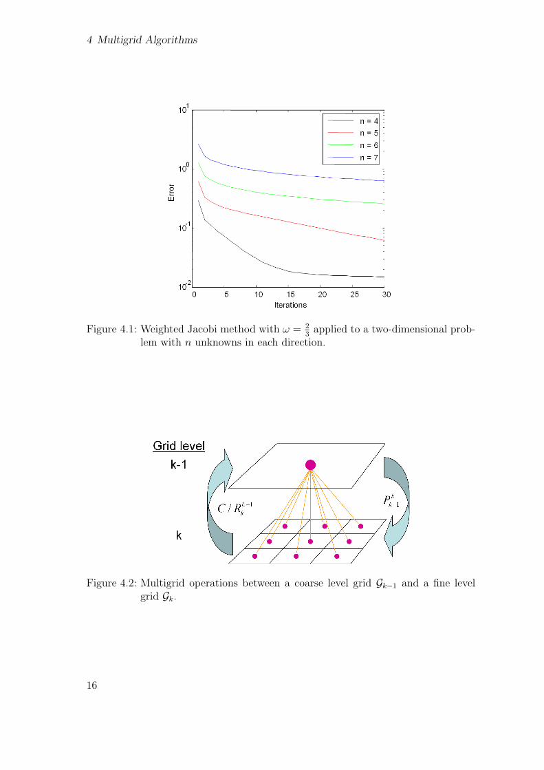
For the Gauss-Seidel and Jacobi iteration scheme, the error reduction rate decreaseswith the number of iterations. The error as a function of the number of iterationsof a weighted Jacobi solver is depicted in Figure 4.1. One can show that the errorreduction rate depends on the error frequency [1]. High frequency errors are elim-inated fast, however low frequency errors are slowly eliminated. At the beginningof a solution process, the error decreases rapidly. The initial decrease correspondsto the quick elimination of high-frequency modes of the error. Low-frequency errormodes remain. This insight is what multigrid algorithms are based on. Here, theidea is that low frequency modes of the error can be treated more efficiently trans-ferring them to coarser grids. If we half the mesh width on a regular grid in 1D,we double the error frequency compared to the fine grid. The idea is to eliminatethe high-frequency error mode with some iterations on the fine grid, and continuethen with iterations on the coarse grid. Thus, the fine grid low-frequency modesare transformed to error modes of higher frequency and can be eliminated moreeffectively.
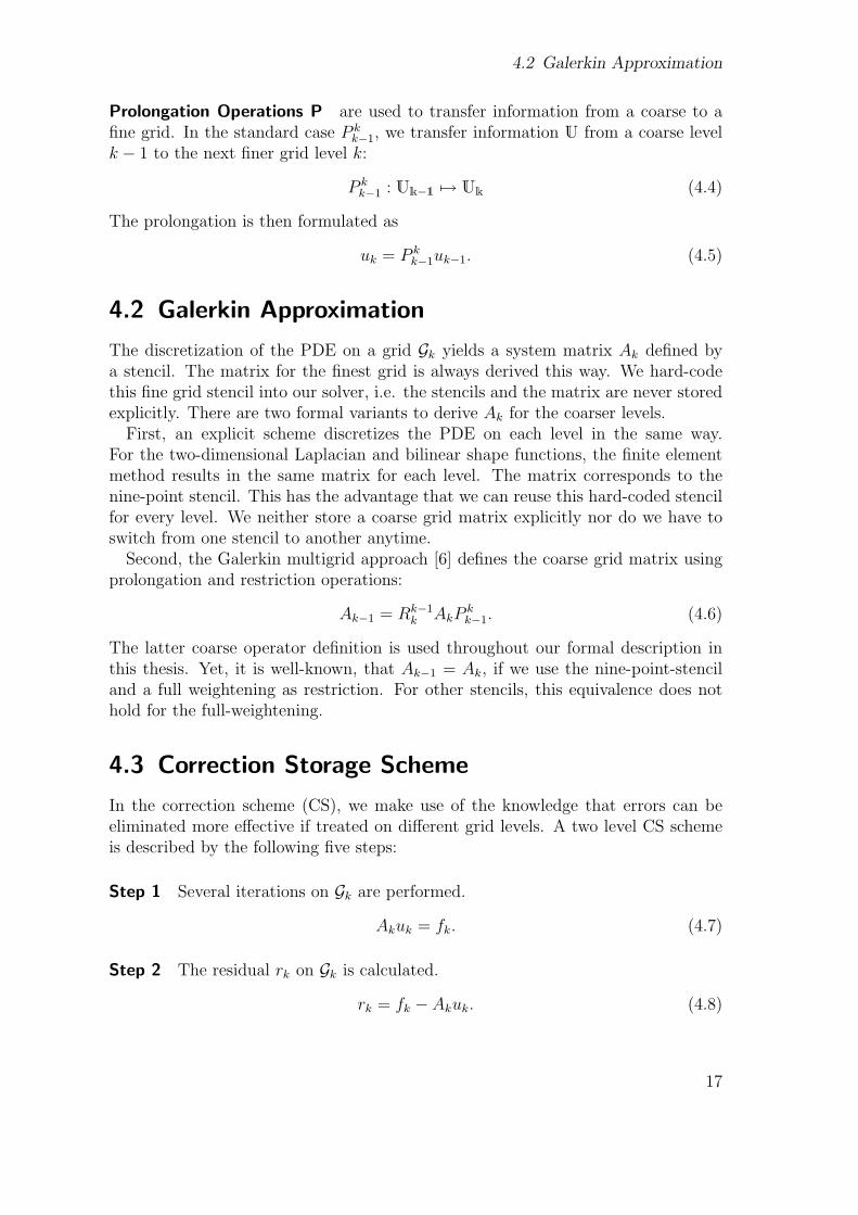
4.1 Multigrid Notations
In multigrid schemes, additional operations to transfer the information between gridlevels are required.
Restriction operations R are used to transfer information to coarser levels. Inthe standard case Rk−1
k , we transfer information U from a fine level k to the nextcoarser level k − 1.
Rk−1k : Uk 7→ Uk−1 (4.1)
The transformation equation is written as
uk−1 = Rk−1k uk. (4.2)
Injection C is the injection operator. The injection is a special case of the restric-tion operations. The transfer of information is done by taking certain values of thefine grid values uk and setting these values without further modification as the newcoarse grid values uk−1. The new notation of the coarse grid values
uk−1 = Cuk (4.3)
highlights that the values are not modified during the transformation.
15
4 Multigrid Algorithms
Figure 4.1: Weighted Jacobi method with ω = 23
applied to a two-dimensional prob-lem with n unknowns in each direction.
Figure 4.2: Multigrid operations between a coarse level grid Gk−1 and a fine levelgrid Gk.
16
4.2 Galerkin Approximation
Prolongation Operations P are used to transfer information from a coarse to afine grid. In the standard case P k
k−1, we transfer information U from a coarse levelk − 1 to the next finer grid level k:
P kk−1 : Uk−1 7→ Uk (4.4)
The prolongation is then formulated as
uk = P kk−1uk−1. (4.5)
4.2 Galerkin Approximation
The discretization of the PDE on a grid Gk yields a system matrix Ak defined bya stencil. The matrix for the finest grid is always derived this way. We hard-codethis fine grid stencil into our solver, i.e. the stencils and the matrix are never storedexplicitly. There are two formal variants to derive Ak for the coarser levels.
First, an explicit scheme discretizes the PDE on each level in the same way.For the two-dimensional Laplacian and bilinear shape functions, the finite elementmethod results in the same matrix for each level. The matrix corresponds to thenine-point stencil. This has the advantage that we can reuse this hard-coded stencilfor every level. We neither store a coarse grid matrix explicitly nor do we have toswitch from one stencil to another anytime.
Second, the Galerkin multigrid approach [6] defines the coarse grid matrix usingprolongation and restriction operations:
Ak−1 = Rk−1k AkP
kk−1. (4.6)
The latter coarse operator definition is used throughout our formal description inthis thesis. Yet, it is well-known, that Ak−1 = Ak, if we use the nine-point-stenciland a full weightening as restriction. For other stencils, this equivalence does nothold for the full-weightening.
4.3 Correction Storage Scheme
In the correction scheme (CS), we make use of the knowledge that errors can beeliminated more effective if treated on different grid levels. A two level CS schemeis described by the following five steps:
Step 1 Several iterations on Gk are performed.
Akuk = fk. (4.7)
Step 2 The residual rk on Gk is calculated.
rk = fk − Akuk. (4.8)
17

4 Multigrid Algorithms
Step 3 rk is restricted to the right hand side of the next coarser grid Gk−1:
fk−1 = Rk−1k rk. (4.9)
The initial guess for the solution of the coarse grid system
Ak−1uk−1 = fk−1 (4.10)
is uk−1 = 0.
Step 4 The system (4.10) is solved. The resulting solution uk−1 is a coarse ap-proximation of the fine grid error ek. Thus, we can reformulate (4.10) to
uk−1 = ek−1 = A−1k−1R
k−1k rk (4.11)
Compared to the fine grid Gk, a direct solution on the coarsened grid requires sig-nificantly less operations. The reason is that the number of unknowns n decreaseson a tri-partitioned grid with
nk−i = nk · 3−d. (4.12)
Step 5 Using the coarse grid estimation of the error from equation (4.11) we canenhance the approximation of the solution on the fine grid
uk = uk + P kk−1uk−1. (4.13)
These steps describe a two-level CS scheme. If we repeat the steps 1-5 recursivelyuntil we reached to the coarsest grid, we end up with the CS multigrid scheme:
if(k=0) then solve Akuk = fk, else
1. Iterate Akuk = fk v1-times.
2. Compute the residual rk = fk − Akuk.
3. Compute fk−1 = Rk−1k rk.
4. Set uk−1 = 0k−1.
5. Apply this scheme recursively.
6. Prolong the error correction to the finer gridsuk = uk + P k
k−1uk−1.
7. Relax Akuk = fk v2 times.
4.4 Full Approximation Storage Scheme
In the previous section, we calculate an error correction on a coarse grid and trans-port it back to the fine grid. For the application of multigrid algorithms on adaptive
18

4.4 Full Approximation Storage Scheme
grids it is useful to have the coarsened fine grid solution available on all levels [17].Thus, the original CS scheme is not well-suited. If we extend CS by a new coarsegrid function
uk−1 = uk−1 + Rk−1k uk, (4.14)
we get a new coarse grid system:
Ak−1uk−1 = fk−1 + Ak−1Rk−1k uk. (4.15)
On this coarse grid, we have now an representation of the coarsened fine grid solutionuk−1. With the modification of the initial guess uk−1 in CS to uk−1, fk−1 has to bemodified accordingly. After these modifications we get to a new scheme, called fullapproximation storage scheme (FAS) [6].
FAS multigrid scheme
if(k=0) then solve Akuk = fk, else
1. Iterate Akuk = fk v1-times.
2. Compute uk−1 = Rk−1k uk.
3. Compute the residual rk = fk − Akuk.
4. Compute fk−1 = Rk−1k rk + Ak−1uk−1.
5. Set uk−1 = uk−1 as initial values on Ωk−1.
6. Apply this scheme γ times.
7. Compute uk = uk + P kk−1(uk−1 − uk−1).
8. Relax Akuk = fk v2 times.
As we can see in step 2, this scheme depends on Rk−1k . However, the FAS scheme is
equivalent to the CS scheme. The reason is the linearity of Rk−1k and the modification
of step 7. If we would choose Rk−1k as a mapping to 0k−1 and choose uk−1 as Rk−1
k uk,we get a CS scheme again.
Compared to the CS, the FAS-MG has a number of advantages [6]:
• With a modification of the coarse grid correction extrapolations, higher orderscan be implemented easily.
• It is applicable to adaptive grids.
• In contrast to CS it can be applied to non-linear problems as well.
One disadvantage of the FAS scheme is, that the required number of calculations ishigher as in the CS scheme [6].
19
4 Multigrid Algorithms
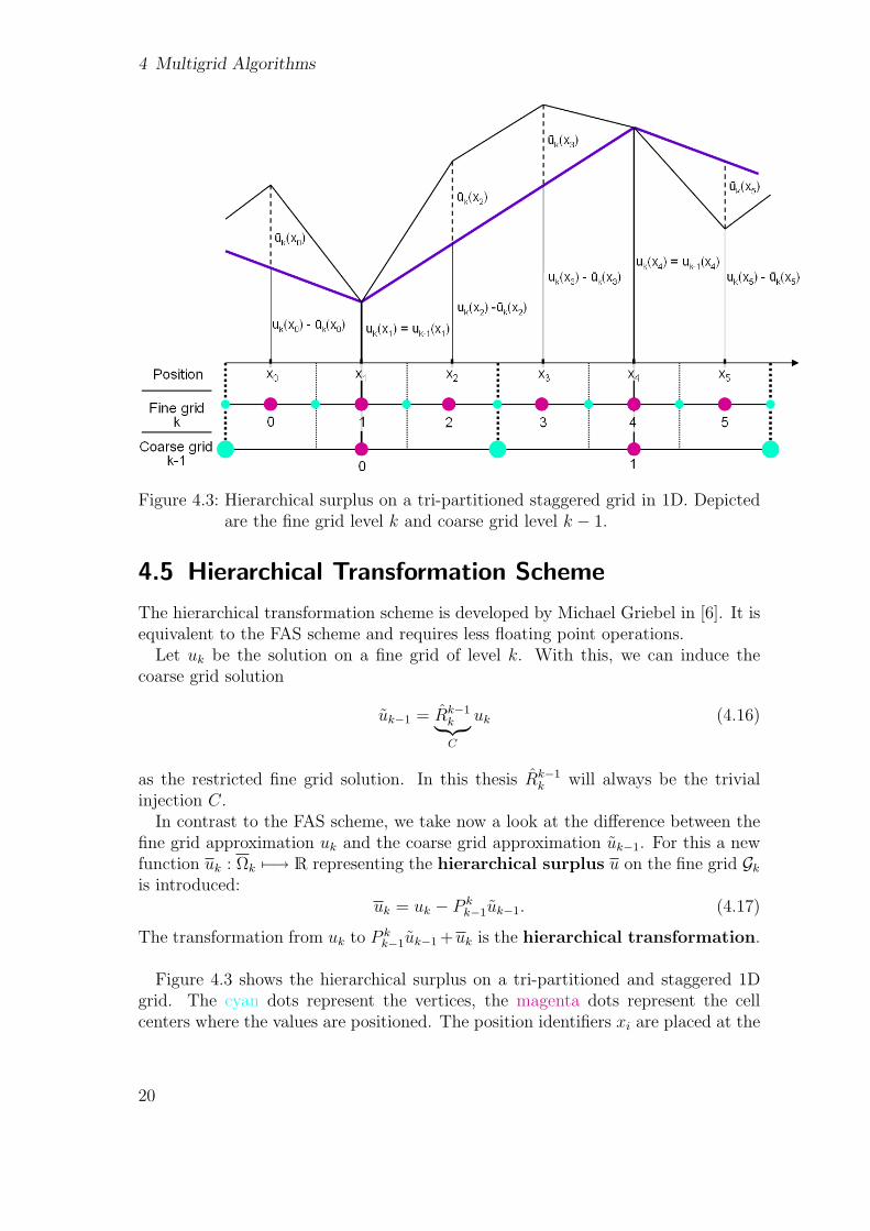
Figure 4.3: Hierarchical surplus on a tri-partitioned staggered grid in 1D. Depictedare the fine grid level k and coarse grid level k − 1.
4.5 Hierarchical Transformation Scheme
The hierarchical transformation scheme is developed by Michael Griebel in [6]. It isequivalent to the FAS scheme and requires less floating point operations.
Let uk be the solution on a fine grid of level k. With this, we can induce thecoarse grid solution
uk−1 = Rk−1k︸ ︷︷ ︸C
uk (4.16)
as the restricted fine grid solution. In this thesis Rk−1k will always be the trivial
injection C.In contrast to the FAS scheme, we take now a look at the difference between the
fine grid approximation uk and the coarse grid approximation uk−1. For this a newfunction uk : Ωk 7−→ R representing the hierarchical surplus u on the fine grid Gk
is introduced:uk = uk − P k
k−1uk−1. (4.17)
The transformation from uk to P kk−1uk−1 +uk is the hierarchical transformation.
Figure 4.3 shows the hierarchical surplus on a tri-partitioned and staggered 1Dgrid. The cyan dots represent the vertices, the magenta dots represent the cellcenters where the values are positioned. The position identifiers xi are placed at the
20

4.5 Hierarchical Transformation Scheme
Figure 4.4: One dimensional FE standard basis function Nki (x) on a staggered grid
Ωk
cell centers. Since we have a tri-partitioned regular grid, one coarse grid cell coversthree fine grid cells. The left vertex of a coarse grid cell is at the same position asthe left vertex of the leftmost inner vertex. The grid is regular. All cells on a certainlevel are of equal size
hk = xi+1 − xi ∀i ∈ N. (4.18)
The values uk(xi) represent the hierarchical surplus at the positions xi depicted bythe dashed lines. The thick purple line represents the linear interpolation function ubetween the coarse grid values uk−1(xi). At the discrete points xi the correspondinginterpolation values uk are calculated. The coarse grid cells ck−1(xi) have the samevalue as their children at the same position ck(xi) had before the hierarchization.Thus,
uk(x1) = uk−1(x1) and (4.19)
uk(x4) = uk−1(x4). (4.20)
In the following, we follow the HT-MG description of Griebel [6, pp. 17-22]. How-ever, we modify certain steps taking into account that we are working on a tri-partitioned staggered grid. Besides this, we use bilinear ansatz functions. These arechosen as a full stencil based smoother is implemented. In case of other stencils,different ansatz functions could be preferable.
We use the well-known 1d hat functions as our standard base functions:
Nki (x) =
x− xi−1
xi − xi−1
: x ∈ [xi−1, xi]
xi+1 − xxi+1 − xi
: x ∈ [xi, xi+1]
0 : x 6∈ [xi−1, xi+1]
(4.21)
The 2d hat function results from a tensor product of the 1d hat functions. TheFigures 4.4 and 4.5 depict the standard base functions Ni(x) on a fine Gk and acoarse Gk−1 grid. We write Nk
i (x) for the standard base function on the fine andNk−1
i (x) on the coarse grid. As we work an a tri-partitioned grid, the base of thebase function Nk−1
i (x) is three times bigger then the base in Gk.
21
4 Multigrid Algorithms
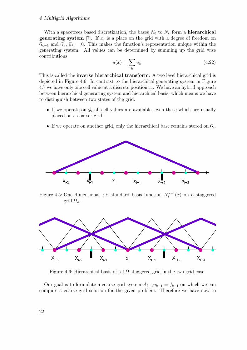
With a spacetrees based discretization, the bases N0 to Nk form a hierarchicalgenerating system [7]. If xi is a place on the grid with a degree of freedom onGk−1 and Gk, uk = 0. This makes the function’s representation unique within thegenerating system. All values can be determined by summing up the grid wisecontributions
u(x) =∑
k
uk. (4.22)
This is called the inverse hierarchical transform. A two level hierarchical grid isdepicted in Figure 4.6. In contrast to the hierarchical generating system in Figure4.7 we have only one cell value at a discrete position xi. We have an hybrid approachbetween hierarchical generating system and hierarchical basis, which means we haveto distinguish between two states of the grid:
• If we operate on Gi all cell values are available, even these which are usuallyplaced on a coarser grid.
• If we operate on another grid, only the hierarchical base remains stored on Gi.
Figure 4.5: One dimensional FE standard basis function Nk−1i (x) on a staggered
grid Ωk.
Figure 4.6: Hierarchical basis of a 1D staggered grid in the two grid case.
Our goal is to formulate a coarse grid system Ak−1uk−1 = fk−1 on which we cancompute a coarse grid solution for the given problem. Therefore we have now to
22

4.5 Hierarchical Transformation Scheme
Figure 4.7: Hierarchical generating system of a 1D staggered grid in the two gridcase.
modify the right hand side of the coarse grid system. Similar to the procedure inthe FAS scheme we restrict the hierarchical fine grid residual Rk−1
k rk and set it asthe coarse grid right hand side fk−1. The single steps to this approach are discussedin the following. If we apply the hierarchical transformation to the fine grid systemAkuk = fk, it can be reformulated as
AkPkk−1Cuk = rk, (4.23)
whereas rk is defined as the hierarchical residual
rk = fk − Akuk. (4.24)
We can interpret the separation uk = P kk−1Cuk + u as base transformation. Con-
trariwise the prolongation P kk−1 can be respected as interpolation by means of the
corresponding hierarchical FE base transformation. The Galerkin multigrid criteriaR = P T and the full stencil gives us the restriction operation
Rk−1k =
(P k
k−1
)T(4.25)
for the restriction of the hierarchical residual r. The application of the restrictionRk−1
k on both sides of equation (4.23)
Rk−1k AkP
kk−1Cuk = Rk−1
k rk, (4.26)
leads us with uk−1 = Cuk to
Rk−1k AkP
kk−1uk−1 = Rk−1
k rk. (4.27)
With Ak−1 = Rk−1k AkP
kk−1 and fk−1 = Rk−1
k rk, the coarse grid system reduces to thestandard FAS:
Ak−1uk−1 = fk−1. (4.28)
This fact enables us to write down the FAS using the hierarchical residual:
23

4 Multigrid Algorithms
Hierarchical transformation multigrid scheme
if(k=0) then solve Akuk = fk, else
1. Iterate Akuk = fk v1-times.
2. Coarse fine grid uk−1 = Cuk.
3. Compute the hierarchical surplus uk = uk −P k
k−1uk−1.
4. Compute the hierarchical residual rk = fk−Akuk.
5. Set the hierarchical residual as new right hand sideon the coarse gridfk−1 = Rk−1
k rk.
6. Set uk−1 = uk−1 as the new coarse grid value.
7. Apply this scheme recursively on Ak−1uk−1 = fk−1
until k = 0.
8. Compute uk = uk + P kk−1uk−1.
9. Iterate Akuk = fk v2-times.This cycle represents the central algorithm of this thesis. It is implemented on a
cell based, tri-partitioned staggered grid.
24

5 Geometry Discretization
Before solving a PDE on an adaptive Cartesian grid, a mapping from the computa-tional domain Ω to our Cartesian grid G has to be defined.
We apply a marker-and-cell approach, i.e. we introduce a function that defines,if a cell is in or outside of the domain. According to the discretization procedurefor space trees the computational domain Ω is embedded into a square. If we go tofiner grid levels Gk, we get vertices
vout = v(xout) ∀xout 6∈ Ω.
In the following, a vertex vout is called outer vertex. On the other hand, we getvertices v(xin) laying inside of the domain (xin ∈ Ω). A cell c is defined as an outercell cout, if it is completely outside of the domain or the computational domain’sboundary intersects it.
Inner Vertex A vertex v is defined as an inner vertex vin, if it is inside the domainΩ and the computational domain’s boundary does not intersect one of thecells ci the vertex v belongs to.
Boundary Vertex A vertex v is defined as boundary vertex vb, if is inside of the Ωand and the computational domain’s boundary does intersect at least one ofthe cells ci the vertex v belongs to.
A cell laying completely inside of the domain Ω is defined as
inner cell, if all vertices of the cell are inner vertices, and as
boundary cell, if one or more vertices of the cell are boundary vertices.
The union of the inner Cin and boundary cells Cb forms the discretized computationaldomain Ωh.
Based on these definitions the geometry discretization scheme can be formulatedby the following three steps:
1. Identify all cells which are outside of the domain or intersected by the domainboundary. All other cells are preliminary set to inner.
2. Identify the types of all vertices v ∈ G depending on their position and currentdefinition of the cells they belong to.
3. Switch all inner cells that are adjacent to a boundary vertex to boundary cells.
An example of domain discretization based on this scheme is depicted in figure 5.1.The colored area highlights the outer region.
25

5 Geometry Discretization
Figure 5.1: Definitions of cell and vertex types.
26

6 HT-MG on Staggered AdaptiveCartesian Grids
In this chapter, we show how the HT-MG scheme is implemented on a cell basedadaptive Cartesian grid.
6.1 Information Transfer Using Bilinear Interpolation
The grid consists of both vertices and cells. Besides the representation of the geom-etry, these data structures are used to store the information for calculations on thegrid as well. The element-wise traversal allows only to access data cell-wise. Thismeans that only the cell, it’s vertices and edges are available in local operations.
Neighbor cell values can’t be used explicitly for calculations. As they are neededfor the calculations, vertices are used to transfer the cell value information amongcells. Within this thesis, this transfer is done via storing the d-linear interpolationvalues mi of neighboring cells on the vertices1. We thus can reconstruct all neighborsvalues ui via the interpolation values mi and the local cell value uloc.
Let’s have a look at the interpolation of the information in 2d. The bilinearinterpolation of the point u(x, y) on a rectangle can be described as follows:
u(x, y) =
(1− x− x0
x1 − x0
)(1− y − y0
y1 − y0
)u0 +(
x− x0
x1 − x0
)(1− y − y0
y1 − y0
)u1 +(
1− x− x0
x1 − x0
)
)(y − y0
y1 − y0
)u2 +(
x− x0
x1 − x0
)(y − y0
y1 − y0
)u3 (6.1)
If we apply equation (6.1) on our equidistant Cartesian grid as depicted in Figure
1Except implementations of discussed in Chapter 7.3.
27
6 HT-MG on Staggered Adaptive Cartesian Grids
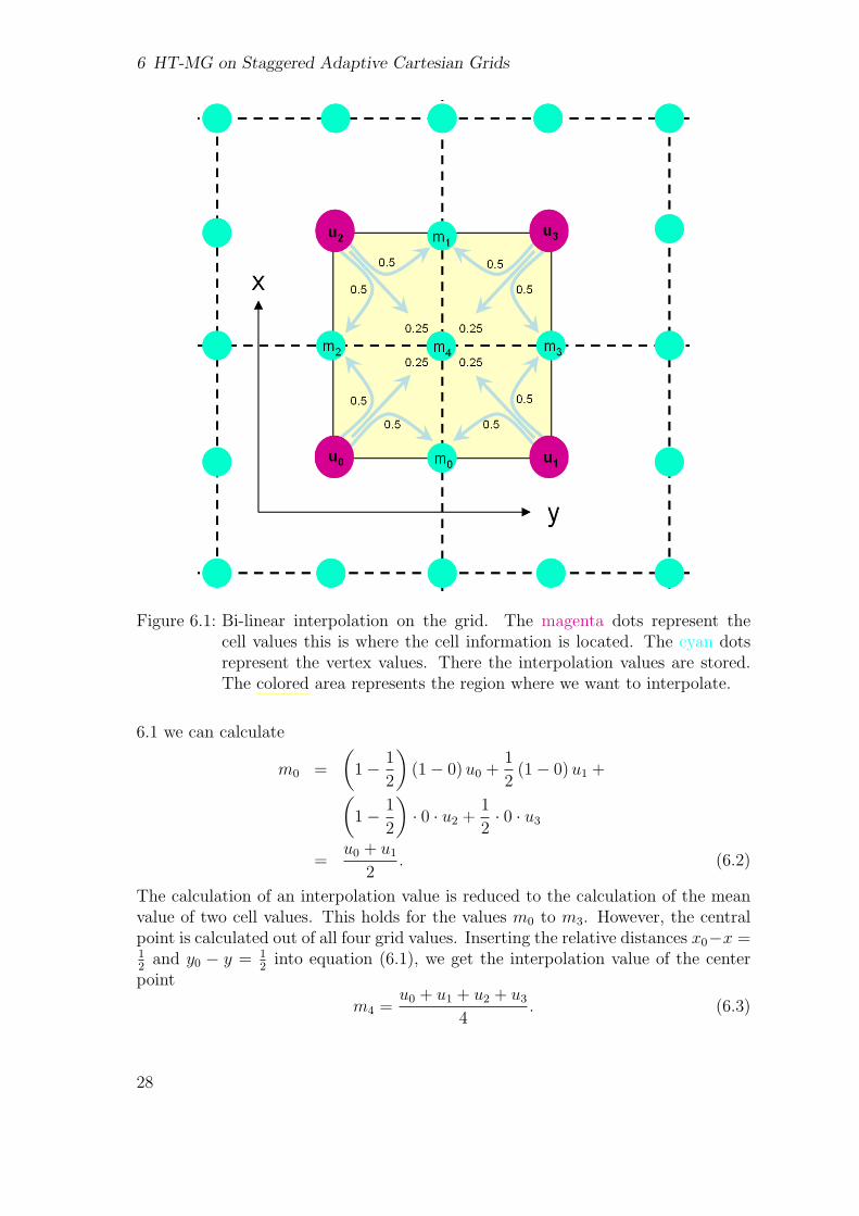
Figure 6.1: Bi-linear interpolation on the grid. The magenta dots represent thecell values this is where the cell information is located. The cyan dotsrepresent the vertex values. There the interpolation values are stored.The colored area represents the region where we want to interpolate.
6.1 we can calculate
m0 =
(1− 1
2
)(1− 0)u0 +
1
2(1− 0)u1 +(
1− 1
2
)· 0 · u2 +
1
2· 0 · u3
=u0 + u1
2. (6.2)
The calculation of an interpolation value is reduced to the calculation of the meanvalue of two cell values. This holds for the values m0 to m3. However, the centralpoint is calculated out of all four grid values. Inserting the relative distances x0−x =12
and y0 − y = 12
into equation (6.1), we get the interpolation value of the centerpoint
m4 =u0 + u1 + u2 + u3
4. (6.3)
28

6.2 Gauss-Seidel on a Cell Based Grid
6.2 Gauss-Seidel on a Cell Based Grid
A full stencil based Gauss-Seidel, like it is presented in this chapter, requires accessto all neighboring cells. The principle of the application of a full stencil is depictedin Figure 6.2(a). As described previously, direct access of neighbor values as it isillustrated by the lines is not possible.
(a) Explicit application of a fullstencil on a grid without restric-tions regarding the neighbor ac-cess.
(b) Implicit application of a fullstencil using the interpolationvalues for the reconstruction ofthe neighbor values.
Figure 6.2: Comparison of stencil application on grids.
Based on the interpolation scheme presented in Chapter 6.1 we will use the inter-polation values to reconstruct the neighbors. The cyan dots in Figure 6.2(b) whichare placed on the edges and vertices of cell 4 represent these values.
Compared to other approaches implemented by Peano, this kind of informationtransfer is new. It has several advantages, which are discussed in Chapter 7.
Step 1: Reconstruct neighbor cell values For the reconstruction of the neighborvalues ui, we use equation (6.2) for axial and (6.3) for diagonal neighbors. Thehighlighted cell in the center of Figure 6.3 represents the active or local cell. Thisis the cell where we are currently working in. To distinguish the local cell valuefrom the reconstructed cell values ui, we call it uloc. The interpolation values mi
and the neighbor cell values ui are enumerated lexicographically from bottom totop. The following equations show the reconstruction calculations corresponding to
29

6 HT-MG on Staggered Adaptive Cartesian Grids
Figure 6.3: Reconstructed cell values
Figure 6.3:
u0 = uloc + 4m0 − 2m1 − 2m3
u1 = 2m1 − uloc
u2 = uloc + 4m2 − 2m1 − 2m4
u3 = 2m3 − uloc
u4 = 2m4 − uloc
u5 = uloc + 4m5 − 2m6 − 2m4
u6 = 2m6 − uloc
u7 = uloc + 4m7 − 2m6 − 2m4 (6.4)
The reconstruction operations can be summarized in a matrix vector operation,which results in the vector u ∈ R8 storing the reconstructed neighbor values. Obvi-ously, the equations (6.4) are linearly independent. Thus, there are several ways tobuild a matrix Mnr representing the operations.
I decided to put the local cell value uloc and the interpolation values mi into avector v ∈ Rd and construct a corresponding transformation matrix Mnr ∈ R8×9:
uneighbors = Mnrv (6.5)
One possible formulation of the matrix is depicted in Annex A.1.
30

6.2 Gauss-Seidel on a Cell Based Grid
Step 2: Calculate the local residual With the reconstructed neighbors, we cannow calculate the local residual rloc, which is used to update the local cell value uloc
in the next step. Furthermore, the local cell values are accumulated to calculate aglobal residual later on.
rloc =1
Ai,i
(f − (Ai,iui +∑
j=0,j 6=i
Ai,j · uj)) (6.6)
The upper matrix based formulation can be transformed into a stencil based nota-tion, which we will use from now on. A, u and f are reordered such that one canaccess grid values as they are represented on a physical domain. In the following, ageneral 2d case is discussed. Therefore we define an abstract full stencil
Astencil =
a6 a7 a8
a3 a4 a5
a0 a1 a2
. (6.7)
With Astencil we now reformulate (6.7) into a stencil based calculation.
rloc =1
a4
f − 3d−1∑j=0
ajuj
(6.8)
Step 3: Update the cell value Based on the general formulation in Chapter 3.6the cell value is updated using rloc from (6.8). For the Gauss-Seidel, we have todivide the residual by the diagonal element, which is the element a4 in AStencil:
ut+1loc = ut
loc + ωrloc
a4
(6.9)
Step 4: Update the interpolation values After step three, the update of the localcell value uloc is completely done. However, we have to take into account that due tothe change of the local cell value the interpolation values mi are outdated and haveto be renewed. The old interpolation values would lead to wrong reconstructionvalues in the neighbors and the algorithm would fail.
The next question is when to update the interpolation value. If this update takesplace after all neighbors have used the interpolation value, the update procedure ina Jacobi scheme. Such a scheme is implemented in [16]. In this implementation, therenewal is done directly after the local cell value update. Hence we get a Gauss-Seidelsolver.
The update procedure of the interpolation values mi is based on Section 6.1. Aninterpolation value is updated by subtracting the weighted old value and adding the
31
6 HT-MG on Staggered Adaptive Cartesian Grids
new cell value:
mk+10 = mk
0 +uk+1
loc − ukloc
4
mk+11 = mk
1 +uk+1
loc − ukloc
2
mk+12 = mk
2 +uk+1
loc − ukloc
4
mk+13 = mk
3 +uk+1
loc − ukloc
2
mk+14 = mk
4 +uk+1
loc − ukloc
2
mk+15 = mk
5 +uk+1
loc − ukloc
4
mk+16 = mk
6 +uk+1
loc − ukloc
2
mk+17 = mk
7 +uk+1
loc − ukloc
4
With this step - the update of the interpolation values - the local smoothing proce-dure is completed and we can enter the next cell.
6.3 Boundary Conditions on Staggered Grids
In the previous section, we have seen how to solve the Poisson equation applying acell-wise Gauss-Seidel. To solve the system, we must specify and handle boundaryconditions as well. According to our cell definitions, the boundary lies always on theedge of our cells. This can be seen in Figure 5.1. In our case, the vertices form thediscrete domain boundaries. Since we work on a staggered grid, these values do notcoincide with the mathematical position of the unknowns (cell values). However,we can use the vertex values to store the boundary values. With the help of theseboundary values and the cell values, we can construct a correct boundary conditionduring the operations on the grid. Construction and reconstruction routines dependon the boundary type.
The vertex status is set according to the geometry information in the initializationof the grid. This is described in Chapter 5. Boundary values are set during theinitialization and must remain unchanged during the calculations.
6.3.1 Dirichlet Boundary Conditions
If we are in a boundary cell, we can not perform a local Gauss-Seidel operation asdescribed in described in Chapter 6.2. In case of Dirichlet boundary conditions, amodification of interpolation value update (Step 4) is necessary. Since we store the
32
6.3 Boundary Conditions on Staggered Grids
interpolation values mi we have to make sure that the Dirichlet vertex values keepthe mathematical initial settings during the calculations: If
u|∂Ω = g(x) ∀x ∈ Ω (6.10)
thenmdirichlet = g(x) x ∈ Ω. (6.11)
This means: If we are in a boundary cell with Dirichlet boundary vertices, we haveto replace the corresponding update equations in step 4 by
mt+1dirichlet = mt
dirichlet. (6.12)
mdirchilet represents the interpolation value on the grid. They remain unchangedduring the operations.
6.3.2 Neumann Boundary Conditions
The Neumann boundary conditions are implemented based on interpolation values,too. Again, the way to store and reconstruct information at these kind of boundarypoints is modified. During the calculations the initial boundary condition
∂y
∂ν(x) = f(x) ∀x ∈ ∂Ω. (6.13)
must be conserved. On our discrete grid this means that if a boundary cell valueut
0 is changed, the corresponding boundary interpolation values must be changed aswell. An axial boundary value mt
∂Ω,axial must be modified such that
ut0 −mt
∂Ω,axial
h=ut+1
0 −mt+1∂Ω,axial
h. (6.14)
For the diagonal boundary values we use the example depicted in Figure 6.4. Asdiagonal Neumann boundary value are defined normal to the boundary, the modi-fication of m∂Ω,diag is formulated with respect to the interpolation value m01. Witha change of ut
0 to ut+10 the modification of m01 is defined as
mt+101 = mt
01 +ut+1
0 − ut0
2. (6.15)
With mt+101 the update of m∂Ω,diag is defined:
mt01 −mt
∂Ω,diag
h=mt+1
01 −mt+1∂Ω,diag
h. (6.16)
The update procedure is depicted in Figure 6.5. Here the boundary cell value ut0 is
changed to ut+10 . From equation (6.14) we can derive the new Neumann boundary
valuemt+1
∂Ω = mt∂Ω + ut+1
0 − ut0. (6.17)
The vertex on the right hand side of cell 0 is an an inner vertex value, which ismodified due to the modification of u0 as well.
33

6 HT-MG on Staggered Adaptive Cartesian Grids
Figure 6.4: Boundary cell with Neumann boundaries.
6.3.3 Modification of the Diagonal Elements
If we are at ∂Ω and want to apply a smoothing step on such a cell, the underlayingmath enforces a modification of the stencil. The same holds for the prolongationor restriction operations, where neighbor values must be reconstructed. This is notdone in this thesis and thus, the behavior of the implemented algorithm is not asone would expect from the theoretical point of view (see Chapter 8).
6.4 Coarsening of a Staggered Grid
The first base function of the HT-MG we will discuss in detail is coarsening. As wework on a tri-partitioned grid, we coarse always a subset of 3d cells on the fine levelto one cell on the coarse level. The coarsening function used is the trivial injectionC:
uk−1 = Cuk. (6.18)
The trivial injection has to be transformed into cell based calculations again. Theprinciple of a cell based injection is depicted in Figure 6.6. Hence the coarse gridcell on the right hand side is the father of the fine grid cells on the left-hand side.
The cell based update procedure can be subdivided in following steps:
Step 1: Transport of the information The center cell value uk,4 of the fine girdcell values uk,i is taken and set as cell value uk−1 on our coarser grid:
uk−1 = uk,4. (6.19)
u stands for the coarsened fine grid solution.
34

6.4 Coarsening of a Staggered Grid
Figure 6.5: Update of a boundary cell value u0 and the corresponding boundaryinterpolation values mt
∂Ω on a 1d grid. The arrows illustrate the changeof the values.
Figure 6.6: Coarsening between two levels
Step 2: Setting the vertex values on the coarse grid Next, we have to updatethe vertex values on the coarse grid. Before the coarsening, all values mi on thecoarse grid Gk−1 are reset to 0.
The coarse grid vertex values are updated applying bilinear interpolation again.This is done according to the procedure presented in Chapter 6.1. We accumulatethe correct interpolation values by summing up the weighted cell values.
In the 2d case, we add one forth of the cells value to the diagonal elements andone half to the axial elements. The calculation of the interpolation values mi of the
35
6 HT-MG on Staggered Adaptive Cartesian Grids
coarsened fine grid solution uk−1 are calculated as follows:
m0 = m0 +uk−1
4
m1 = m1 +uk−1
2
m2 = m2 +uk−1
4
m3 = m3 +uk−1
2
m4 = m4 +uk−1
2
m5 = m5 +uk−1
4
m6 = m6 +uk−1
2
m7 = m7 +uk−1
4
6.5 Calculation of the Hierarchical Surplus
For the calculation of the hierarchical surplus uk, we prolong all coarsened fine gridvalues uk−1 to the fine grid via bilinear interpolation and subtract these from thefine grid values. For the bilinear interpolation the prolongation operator P k
k−1 isused:
uk = uk − P kk−1u
k−1 (6.20)
According to the region covered by the coarse grid hat one cell value affects 7d
neighbor values. P1d,complete is the prolongation stencil for the 1d case:
P1d,complete =[0 1
323
1 23
13
0]
We can see that the neighbors at the ends of the stencil are weighted with 0. Thisholds for higher dimensions too and allows us to reduce the prolongation stencil toa 5d stencil. P2d is the stencil for the 2d case:
P2d =1
9
1 2 3 2 12 4 6 4 23 6 9 6 32 4 6 4 21 2 3 2 1
(6.21)
Step 1: Compute hierarchical surplus As we see in (6.20), we have to subtractP k
k−1uk−1 from the fine grid values. For this, we need the neighbors of the current
coarse grid cell. Due to the Peano framework, we have the restriction that we canonly access one parent cell and its next level children [17]. Here, the interpolation
36

6.5 Calculation of the Hierarchical Surplus
values which were set in second step of the coarsening come into operation. We usethem to reconstruct the neighbor cells uk−1,i on the coarse grid. Using these values,we are able to compute the hierarchical surplus on the children cells. At first, wereconstruct the coarse grid neighbors as described in Chapter 6.2, step 1:
uk−1,0 = uk−1 + 4mk−1,0 − 2mk−1,1 − 2mk−1,3
uk−1,1 = 2mk−1,1 − uk−1
uk−1,2 = uk−1 + 4mk−1,2 − 2mk−1,1 − 2mk−1,4
uk−1,3 = 2mk−1,3 − uk−1
uk−1,4 = 2mk−1,4 − uk−1
uk−1,5 = uk−1 + 4mk−1,5 − 2mk−1,6 − 2mk−1,4
uk−1,6 = 2mk−1,6 − uk−1
uk−1,7 = uk−1 + 4mk−1,7 − 2mk−1,6 − 2mk−1,4
With the prolongation stencil P2d we can now calculate the hierarchical surplus u(2d):
uk = uk − P2duk−1 (6.22)
uk,0
uk,1
uk,2
uk,3
uk,4
uk,5
uk,6
uk,7
uk,8
=
uk,0
uk,1
uk,2
uk,3
uk,4
uk,5
uk,6
uk,7
uk,8
− 1
9
1 2 0 2 4 0 0 0 00 3 0 0 6 0 0 0 00 2 1 0 4 2 0 0 00 0 0 3 6 0 0 0 00 0 0 0 9 0 0 0 00 0 0 0 6 3 0 0 00 0 0 2 4 0 1 2 00 0 0 0 6 0 0 3 00 0 0 0 4 2 0 2 1
︸ ︷︷ ︸
P2d
uk−1,0
uk−1,1
uk−1,2
uk−1,3
uk−1,4
uk−1,5
uk−1,6
uk−1,7
uk−1,8
The hierarchical surplus set to the corresponding cells on the fine grid.
Step 2: Compute interpolation values of hierarchical surplus This step is nec-essary because we must compute the hierarchical residual out of the hierarchicalsurplus. Due to our cell based grid, this is only possible, if we set interpolationvalues accordingly. After the calculation of the hierarchical surplus, we have tocompute the interpolation values mi of the hierarchical values u. For the procedurebelow, we assume that all inner vertex values on the fine grid were reset to 0 beforewe start the update.
In the previous section, we have seen that the interpolation values are computedby bilinear interpolation. Basically, we apply the same strategy here. We use an in-terpolation matrix M ir (subscript ir stands for ”interpolation value reconstruction”)to map the hierarchical surplus values u to their interpolation values m:
m = M iru. (6.23)
37

6 HT-MG on Staggered Adaptive Cartesian Grids
Here, we do that on our subset of 9 cells and 40 interpolation values. This meansthat M ir ∈ R9×40. Similar to step 2 of the coarsening the interpolation values at
Figure 6.7: Interpolation of the hierarchical surplus
the boundary of our subset are not completely updated after we finished this localprocedure. The reason is that
mboundary = g(u ∈ ck vchild ck−1 u u ∈ ck 6vchild ck−1). (6.24)
Whereas all inner vertex values are fully defined by
minner = g(u ∈ ck vchild ck−1). (6.25)
The contributions of neighbor cells are missing. Figure 6.7 depicts the subset of finegrid cells. All inner vertex values are completely updated when equation (6.23) isapplied.
6.6 Computing the Hierarchical Residual
For the computation of the hierarchical residual
rk = fk − Akuk (6.26)
on our cell based grid, we use the principles presented with the Gauss-Seidel solverin in Chapter 6.2.
Step 1: Reconstruction of neighbor cells At first, we have to reconstruct the allcell values ui using the interpolation values of the hierarchical surplus mi calculatedin Chapter 6.5. The reconstruction procedure matches the reconstruction step 1described in the previous Section 6.2. It is omitted here.
38
6.7 Restriction of the Hierarchical Residual
Step 2: Calculation of the hierarchical residual Having the neighbor cell valuesreconstructed, we can calculate the hierarchical residual as follows:
rk+1loc =
1
a4
(f −3d−1∑j=0
ajuj) (6.27)
aj are again the values from our stencil (6.21). The right hand side f remainsunchanged.
6.7 Restriction of the Hierarchical Residual
For the restriction of the hierarchical residual r to the right hand side of the coarsegrid
fk−1 = Rk−1k uk,
the Galerkin approximation criterion
Rk−1k =
(P k
k−1
)T(6.28)
must hold.If we take a look at our prolongation stencil (6.21), we see that it is symmetric.
As a consequence, the prolongation matrix P kk−1 must be symmetric as well and we
can use the stencil directly as the restriction operator
R2d =(P k
k−1
)T= (P2d)T =
1
9
1 2 3 2 12 4 6 4 23 6 9 6 32 4 6 4 21 2 3 2 1
. (6.29)
The values of R2d give us the weights of the hierarchical residual values rk,i. Thestencil R2d is a 5d stencil. Thus, for the calculation of fk−1 the hierarchical residualvalues rk of 5d cells ck are required. The standard operations of our grid provideonly access to the 3d cells ck vchild ck−1. As a result we can not directly access theresidual values at the boundary of the stencil. This problem is solved by storingthe interpolation values of the hierarchical residual mr in the vertices. Using thesevalues we can reconstruct the neighbor residual values similar to the cell values u.In Figure 6.8 we see the grid elements participating at the reconstruction. The col-ored area represents the the coarse grid cell, respectively highlights the area of itschildren ck vchild ck−1. The values represent the cells ck 6vchild ck−1. They are notaccessible directly.
The residual values rk of these cells are reconstructed using the interpolationvalues mr at the boundary of our subset. The reconstruction equations are similarto previous reconstructions based on bilinear interpolated values and are omitted
39

6 HT-MG on Staggered Adaptive Cartesian Grids
Figure 6.8: Reconstruction of the hierarchical residual values
here. They can be summarized to a matrix-vector operation. Based on the equationsin Chapter 6.1 the matrix Mrr ∈ R4d×(4d+3d) (rr = reconstruct residual) is set up.The reconstruction vector vrr ∈ R4d+3d
is built of
• the interpolation values of the hierarchical residual mr for the 4d not directlyaccessible values,
• and the 3d residual values of the cells ck vchild ck−1.
The reconstructed hierarchical residual values are stored in an vector r∗ ∈ R4d:
r∗ = Mrrvrr (6.30)
With these r∗ and the residual values we have from the local fine grid cells, we canapply the restriction. For this we store all residual values in a vector r. With (6.29)and r we compute
fk−1 =5D−1∑i=0
ripi. (6.31)
The coarse grid right hand side fk−1 is available. For the whole algorithm this meansthat Ak−1uk−1 = fk−1 is completely defined.
6.8 Inverse Hierarchical Transformation
The procedure is similar to the hierarchization. For the calculation of the new finegrid value uk we prolong the approximated solution on the coarse grid uk−1 to the
40

6.8 Inverse Hierarchical Transformation
fine grid via bilinear interpolation and add these to the hierarchized fine grid valuesuk−1:
uk = uk + P kk−1uk−1 (6.32)
For the bilinear interpolation the prolongation operator P kk−1, respectively the pro-
longation stencil (6.21) is used.The reconstruction of the coarse grid neighbors equals the previous reconstruc-
tions.
uk−1,0 = uk−1 + 4mk−1,0 − 2mk−1,1 − 2mk−1,3
uk−1,1 = 2mk−1,1 − uk−1
uk−1,2 = uk−1 + 4mk−1,2 − 2mk−1,1 − 2mk−1,4
uk−1,3 = 2mk−1,3 − uk−1
uk−1,4 = 2mk−1,4 − uk−1
uk−1,5 = uk−1 + 4mk−1,5 − 2mk−1,6 − 2mk−1,4
uk−1,6 = 2mk−1,6 − uk−1
uk−1,7 = uk−1 + 4mk−1,7 − 2mk−1,6 − 2mk−1,4
With the prolongation stencil P2d we can now calculate the dehierarchized fine gridvalues uk (2d):
uk = uk + P2duk−1 (6.33)
uk,0
uk,1
uk,2
uk,3
uk,4
uk,5
uk,6
uk,7
uk,8
=
uk,0
uk,1
uk,2
uk,3
uk,4
uk,5
uk,6
uk,7
uk,8
+
1
9
1 2 0 2 4 0 0 0 00 3 0 0 6 0 0 0 00 2 1 0 4 2 0 0 00 0 0 3 6 0 0 0 00 0 0 0 9 0 0 0 00 0 0 0 6 3 0 0 00 0 0 2 4 0 1 2 00 0 0 0 6 0 0 3 00 0 0 0 4 2 0 2 1
︸ ︷︷ ︸
P2d
uk−1,0
uk−1,1
uk−1,2
uk−1,3
uk−1,4
uk−1,5
uk−1,6
uk−1,7
uk−1,8
After the computation of the solution on the coarsest grid G0 we start to descend in
the grid. In the descent we have apply two operations, inverse hierarchical transformand postsmoothing. As the postsmoothing is nothing but another GS smoothingstep it is not described separately.
41

6 HT-MG on Staggered Adaptive Cartesian Grids
42
7 Challenges and Technical Solutions
In the previous section we have seen how the HT-MG is implemented on staggeredgrids. In this chapter the technical details of the implementation are explained.
7.1 The Peano Framework
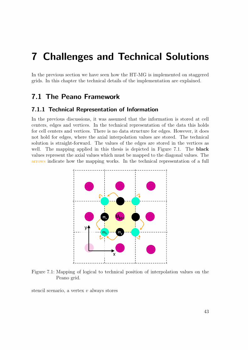
7.1.1 Technical Representation of Information
In the previous discussions, it was assumed that the information is stored at cellcenters, edges and vertices. In the technical representation of the data this holdsfor cell centers and vertices. There is no data structure for edges. However, it doesnot hold for edges, where the axial interpolation values are stored. The technicalsolution is straight-forward. The values of the edges are stored in the vertices aswell. The mapping applied in this thesis is depicted in Figure 7.1. The blackvalues represent the axial values which must be mapped to the diagonal values. Thearrows indicate how the mapping works. In the technical representation of a full
Figure 7.1: Mapping of logical to technical position of interpolation values on thePeano grid.
stencil scenario, a vertex v always stores
43

7 Challenges and Technical Solutions
• the diagonal interpolation values md at the position of the vertex,
• the next upper interpolation value mx, and
• the next right interpolation value my.
The indices d, x and y stand for the direction of the interpolation value. Besides,the vertex holds
• states of the interpolation values mi,
• residual interpolation values (in HT-MG), and
• further grid related information, which is omitted here.
In some functions, the state of the vertex is required. Here, we determine the stateby the state of the diagonal interpolation value.
Cells c store
• the solution u,
• the residual r,
• the right hand side f ,
• the cell state, and
• further grid related information, which is omitted here.
7.1.2 Grid Initialization
The UML class diagram in Figure 7.2 shows the elementary dependencies of the gridcreation. The configuration of vertices and cells depends on the chosen stencil andscenario. For each scenario-stencil tuple a corresponding adapter is written. Thisadapter is called by the grid initialization routines. The initialization is done via anelement-wise grid traversal.
At this initialization traversal an initialization adapter has to provide the followingtwo functions:
createDegreeOfFreedom(vertex) initializes the grid’s vertices. The following val-ues/states are initialized:
• The interpolation values mi.
• Interpolation value state.
createDegreeOfFreedom(cell) initializes the grid’s cell. The following values/s-tates of the cell are initialized:
• Cell value u.
• Right hand side f .
• Cell state.
44

7.1 The Peano Framework
Figure 7.2: Simplified UML class diagram of the grid creation.
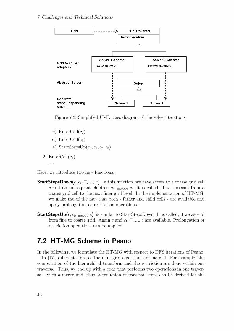
7.1.3 Grid Operations for Solvers
Again the operations are integrated into the functions of Peano. The class diagramin Figure 7.3 shows the call hierarchy of a solution process. The grid iteration callsthe functions of a solver specific adapter. This adapter calls then the correspondingfunction in a solver. For the application of GS we use the following function of thegrid:
EnterCell(cell,vertices) is called each time a new cell is entered.
In this function, we have access to one cell and the corresponding vertices. Eachtime the function is called, we apply the local GS scheme as described in chapter6.2. Obviously, we have to define a grid level on which we want to solve the system.If a GS is used as a direct solver it is only applied on the leaves.
To apply the HT-MG, functions for the transfer of information are needed. How-ever, it is worth while to take a look at technical realization of the traversal scheme.In Chapter 3.3 it is described that we traverse the grid in a depth-first-search man-ner. This means after entering a coarse grid cell c all cj vchild c are traversed. Thisphase is called descent. If the finest grid is reached, we ascend until we reach toc again. This phase is called ascent. Now the next cell on level k is entered andthe descent there begins. This procedure is depicted in Figure 7.4. The follow-ing sequence shows a part of the function calls, which are called the grid during atraversal. We refer to the traversal depicted in Figure 7.4:
1. EnterCell(c0)
a) StartStepsDown(c0, c1, c2, c3)
b) EnterCell(c1)
45
7 Challenges and Technical Solutions
Figure 7.3: Simplified UML class diagram of the solver iterations.
c) EnterCell(c2)
d) EnterCell(c3)
e) StartStepsUp(c0, c1, c2, c3)
2. EnterCell(c1). . .
Here, we introduce two new functions:
StartStepsDown(c, ck vchild c) In this function, we have access to a coarse grid cellc and its subsequent children ck vchild c. It is called, if we descend from acoarse grid cell to the next finer grid level. In the implementation of HT-MG,we make use of the fact that both - father and child cells - are available andapply prolongation or restriction operations.
StartStepsUp(c, ck vchild c) is similar to StartStepsDown. It is called, if we ascendfrom fine to coarse grid. Again c and ck vchild c are available. Prolongation orrestriction operations can be applied.
7.2 HT-MG Scheme in Peano
In the following, we formulate the HT-MG with respect to DFS iterations of Peano.In [17], different steps of the multigrid algorithm are merged. For example, the
computation of the hierarchical transform and the restriction are done within onetraversal. Thus, we end up with a code that performs two operations in one traver-sal. Such a merge and, thus, a reduction of traversal steps can be derived for the
46

7.2 HT-MG Scheme in Peano
Figure 7.4: Cell traversal order of a two level grid. The number with brackets rep-resent the corresponding step in the function call sequence described inthe text. Those without brackets represent the Peano traversal order ofthe elements, illustrated by the arrows as well.
staggered Poisson solver, too. The complete traversal scheme is described in thefollowing tabular:
Iteration Algorithmstate / Peanofunction
Algorithm Operation
1
Descent /EnterCell
Step 1: SmoothingApply the smoothing scheme on Gk. Update the in-terpolation values mk accordingly.In this function, we use
• uk, and
• mk.
Ascent /StartStepsUp
Step 2: CoarseningIf it is the last smoothing iteration on Gk, applyuk−1 = Cuk and update the coarse grid interpolationvalues mk−1 accordingly.
47

7 Challenges and Technical Solutions
Iteration Algorithmstate / Peanofunction
Algorithm Operation
2
Descent /StartStepsDown
Step 3: Hierarchical surplusCompute the hierarchical surplus uk = uk−P k
k−1uk−1
and update the fine grid interpolation values mk ac-cordingly. As we can reconstruct the fine grid val-ues, the values uk and mk are not needed any longer.Therefore we overwrite these values with uk and mk.In this function, we use
• uk−1,
• mk−1, and
• uk.
Ascent No HT-MG operation.
3
Descent Step 4: Hierarchical residualCompute rk = fk − Akuk and set mrr,k accordingly.At this step the residual rk is not needed anymore.Instead of using different variables we overwrite rk =rk.In this function, we use
• uk, and
• mk.
Ascent No HT-MG operation.
48
7.2 HT-MG Scheme in Peano
Iteration Algorithmstate / Peanofunction
Algorithm Operation
4
Descent Step 5: Restriction of the hierarchical residualRestrict the hierarchical residual fk−1 = Rk−1
k rk. Af-ter this step, the values mrr,k are not needed forfurther calculations. The required memory is freed.Now, the coarse grid system Ak−1uk−1 = fk−1 is de-fined and steps 1-5 are repeated recursively until G0
is reached. If it is reached, we go to the next step.In this function, we use
• rk, and
• mrr,k.
Ascent No HT-MG operation.
5
Descent Step 6: Inverse hierarchical transformCompute uk = uk +P k
k−1uk−1 and set mk accordingly.In this function, we use
• uk−1, and
• mk−1.
Ascent No HT-MG operation.
6
Descent Step 7: PostsmoothingApply the smoothing scheme on Gk. Update the in-terpolation values mk accordingly.In this function, we use
• uk, and
• mk.
Ascent No HT-MG operation.
Table 7.1: HT-MG implementation in the Peano framework
It takes five grid traversals to complete one level update. As the spacetree traver-sals itself are rather costly, one would prefer to merge steps. For several operationsthis is not possible.
A closer look at step 3 and 4 shows why it is not applicable in many cases.
49
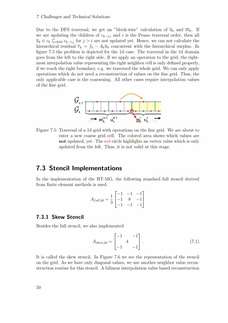
7 Challenges and Technical Solutions
Due to the DFS traversal, we get an ”block-wise” calculation of uk and mk. Ifwe are updating the children of ck−1,i and i is the Peano traversal order, then alluk ∈ ck vchild ck−1,j for j > i are not updated yet. Hence, we can not calculate thehierarchical residual rk = fk − Akuk concurrent with the hierarchical surplus. Infigure 7.5 the problem is depicted for the 1d case. The traversal in the 1d domaingoes from the left to the right side. If we apply an operation to the grid, the right-most interpolation value representing the right neighbor cell is only defined properly,if we reach the right boundary, e.g. we traversed the whole grid. We can only applyoperations which do not need a reconstruction of values on the fine grid. Thus, theonly applicable case is the coarsening. All other cases require interpolation valuesof the fine grid.
Figure 7.5: Traversal of a 1d grid with operations on the fine grid. We are about toenter a new coarse grid cell. The colored area shows which values arenot updated, yet. The red circle highlights an vertex value which is onlyupdated from the left. Thus, it is not valid at this stage.
7.3 Stencil Implementations
In the implementation of the HT-MG, the following standard full stencil derivedfrom finite element methods is used:
Afull,2d =1
3
−1 −1 −1−1 8 −1−1 −1 −1
7.3.1 Skew Stencil
Besides the full stencil, we also implemented
Askew,2d =
−1 −14
−1 −1
. (7.1)
It is called the skew stencil. In Figure 7.6 we see the representation of the stencilon the grid. As we have only diagonal values, we use another neighbor value recon-struction routine for this stencil. A bilinear interpolation value based reconstruction
50

7.3 Stencil Implementations
Figure 7.6: The vertices and cell needed for the application of the skew stencil.
would require the full neighbor reconstruction scheme as it is presented in Chapter6.2. This is a waste of storage as the axial values are not needed for the calculation.
For the skewed stencil, we hence use only mean values between local cell uloc andneighbor values ui. Thus, the interpolation values are constructed as follows:
m0 =uloc + u0
2(7.2)
m1 =uloc + u1
2(7.3)
m2 =uloc + u2
2(7.4)
m3 =uloc + u3
2(7.5)
The reconstruction is obvious and thus omitted here. However, one has to take intoaccount that if the stencil should be applied in a multigrid scheme, the multigridoperations may require the axial values as well. In that such a case one would applythe principles presented with the full stencil application.
7.3.2 Standard Stencil
The stencil
Astd,2d =
−1−1 4 −1
−1
(7.6)
is derived from finite differences methods. As we can see in Figure 7.7 only axialinterpolation values are required for the reconstruction of neighbor values. If usedas an iterative solver stencil on staggered grids, we can omit the diagonal values and
51
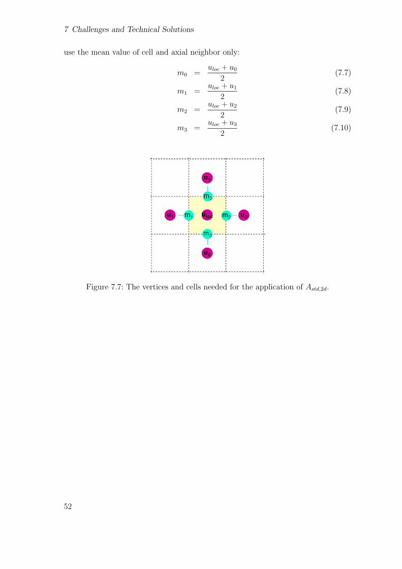
7 Challenges and Technical Solutions
use the mean value of cell and axial neighbor only:
m0 =uloc + u0
2(7.7)
m1 =uloc + u1
2(7.8)
m2 =uloc + u2
2(7.9)
m3 =uloc + u3
2(7.10)
Figure 7.7: The vertices and cells needed for the application of Astd,2d.
52

8 Numerical Experiments
8.1 Test Scenarios
8.1.1 Sinus
The sinus test scenario is a test scenario with homogenous Dirichlet boundary con-ditions on the unit square. The PDE is defined as
−∆u = dπ2Πdi=1 sin(πxi). (8.1)
This scenario is chosen as the analytical solution is known. It is
u = Πdi=1 sin(πxi). (8.2)
In Figure 8.1, we see the the h2-scaled right hand side f . The grid is initialized asfollows:
• u0 = 0.
• f = −h2dπ2 sin(πx)u.1
• u ∈ ∂Ω = 0.
The corresponding solution is depicted in Figure 8.2.
8.1.2 Increased Activity
This scenario was developed by Prof. Ruede [14]. It is a Dirichlet boundary valueproblem on the unit square and has inhomogeneous boundary conditions. The ideais to preset the solution values
g = u =cos(2π(
x+12− y+1
2
))sin(2π(
x+12− y+1
2
))sinh(8π)
(8.3)
on the boundary. The grid is initialized as follows:
• u0 = 0.
• f = 0.
• u ∈ ∂Ω = g.
The solution of the problem is depicted in Figure 8.3.
1The right hand side is always stored pre-scaled in the cells. Thus we must not calculate f · h2
in each update of u.
53
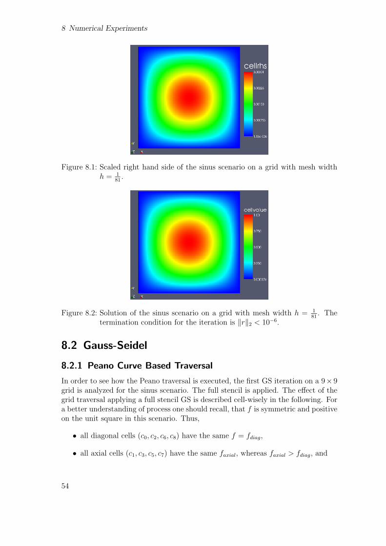
8 Numerical Experiments
Figure 8.1: Scaled right hand side of the sinus scenario on a grid with mesh widthh = 1
81.
Figure 8.2: Solution of the sinus scenario on a grid with mesh width h = 181
. Thetermination condition for the iteration is ‖r‖2 < 10−6.
8.2 Gauss-Seidel
8.2.1 Peano Curve Based Traversal
In order to see how the Peano traversal is executed, the first GS iteration on a 9× 9grid is analyzed for the sinus scenario. The full stencil is applied. The effect of thegrid traversal applying a full stencil GS is described cell-wisely in the following. Fora better understanding of process one should recall, that f is symmetric and positiveon the unit square in this scenario. Thus,
• all diagonal cells (c0, c2, c6, c8) have the same f = fdiag,
• all axial cells (c1, c3, c5, c7) have the same faxial, whereas faxial > fdiag, and
54

8.2 Gauss-Seidel
Figure 8.3: Solution of the increased activity scenario on a grid with mesh widthh = 1
81. The termination condition for the iteration is ‖r‖2 < 10−6.
• the cell c4 has a value fcenter > faxial > fdiag.
From the scenario definitions in Chapter 8.1.1 we now, that all values u = 0 beforethey are updated in the first iterations. If ω = 1.0, then we can simplify the updatein the first iteration to
ut+1loc =
3
8
(f +
1
3
∑uNeighbors
). (8.4)
Due to the zero-initialized domain and the Dirichlet boundary the boundary valuesdo not contribute to the initial update.
Hence, we can conclude that the non-uniform value distribution in Figure 8.4 isa result of the information transport of GS. If we take a look at the grid events wecan document the traversal as follows:
1. EnterCell(c0): No contribution of neighbors. u0 = 38fdiag.
2. EnterCell(c1): c0 was updated in the previous step. It is a neighbor of c1. Wecalculate u1 = 3
8(faxial + 1
3u0).
3. EnterCell(c2): c1 was updated in the previous step. It is a neighbor of c2. Wecalculate u2 = 3
8(fdiag + 1
3u1).
4. EnterCell(c3): Here we have two updated neighbors: c1 and c2. Hence, u3 =38(faxial + 1
3(u1 + u2)). As a result u3 > u1.
This can be seen by a look at the colors expressing the values in Figure 8.4. Atraversal with the same predefinitions on a finer grid is depicted in Figure 8.5.
55

8 Numerical Experiments
Figure 8.4: One Gauss-Seidel iteration on a 3× 3 grid.
8.2.2 Relaxed Gauss-Seidel
In Figure 8.4 we see the results of an omega variation. The underlaying scenario isthe sinus scenario. From theory we know that for a certain PDE GS should show andiscretization independent ωopt. In our case the relaxation behavior is wrong. Thisis due to the fact that the weightening of the diagonal element is not changed at thedomain boundary. The coarser the grid, the bigger the influence of wrong boundaryvalues.
8.3 HT-MG Convergence Analysis
For scenarios as the sinus scenario, we expect that a multigrid algorithms shows aconvergence rate which is nearly independent of the number of unknowns. In figure8.7, we see the convergence rates of our HT-MG for the sinus scenario. The residualvalues as a function of the number of iterations are very close to each other forsignificant different number of unknowns. This is what we would expect. However,the convergence rate seems to be to low.
56
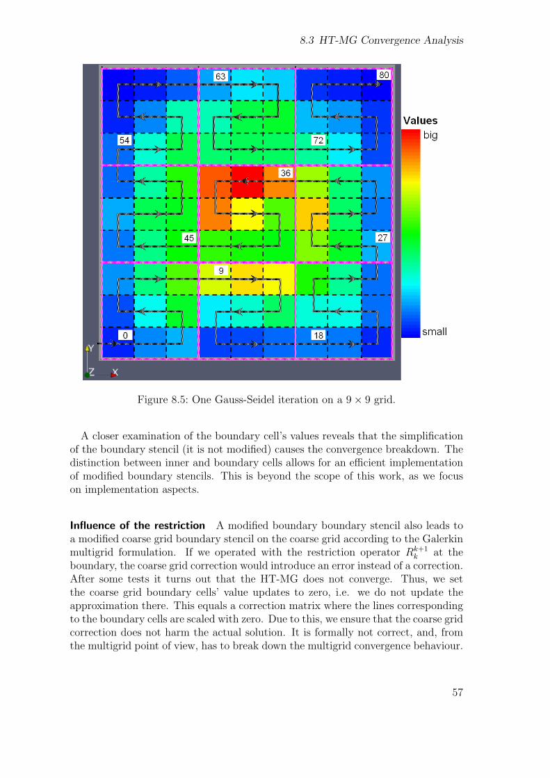
8.3 HT-MG Convergence Analysis
Figure 8.5: One Gauss-Seidel iteration on a 9× 9 grid.
A closer examination of the boundary cell’s values reveals that the simplificationof the boundary stencil (it is not modified) causes the convergence breakdown. Thedistinction between inner and boundary cells allows for an efficient implementationof modified boundary stencils. This is beyond the scope of this work, as we focuson implementation aspects.
Influence of the restriction A modified boundary boundary stencil also leads toa modified coarse grid boundary stencil on the coarse grid according to the Galerkinmultigrid formulation. If we operated with the restriction operator Rk+1
k at theboundary, the coarse grid correction would introduce an error instead of a correction.After some tests it turns out that the HT-MG does not converge. Thus, we setthe coarse grid boundary cells’ value updates to zero, i.e. we do not update theapproximation there. This equals a correction matrix where the lines correspondingto the boundary cells are scaled with zero. Due to this, we ensure that the coarse gridcorrection does not harm the actual solution. It is formally not correct, and, fromthe multigrid point of view, has to break down the multigrid convergence behaviour.
57
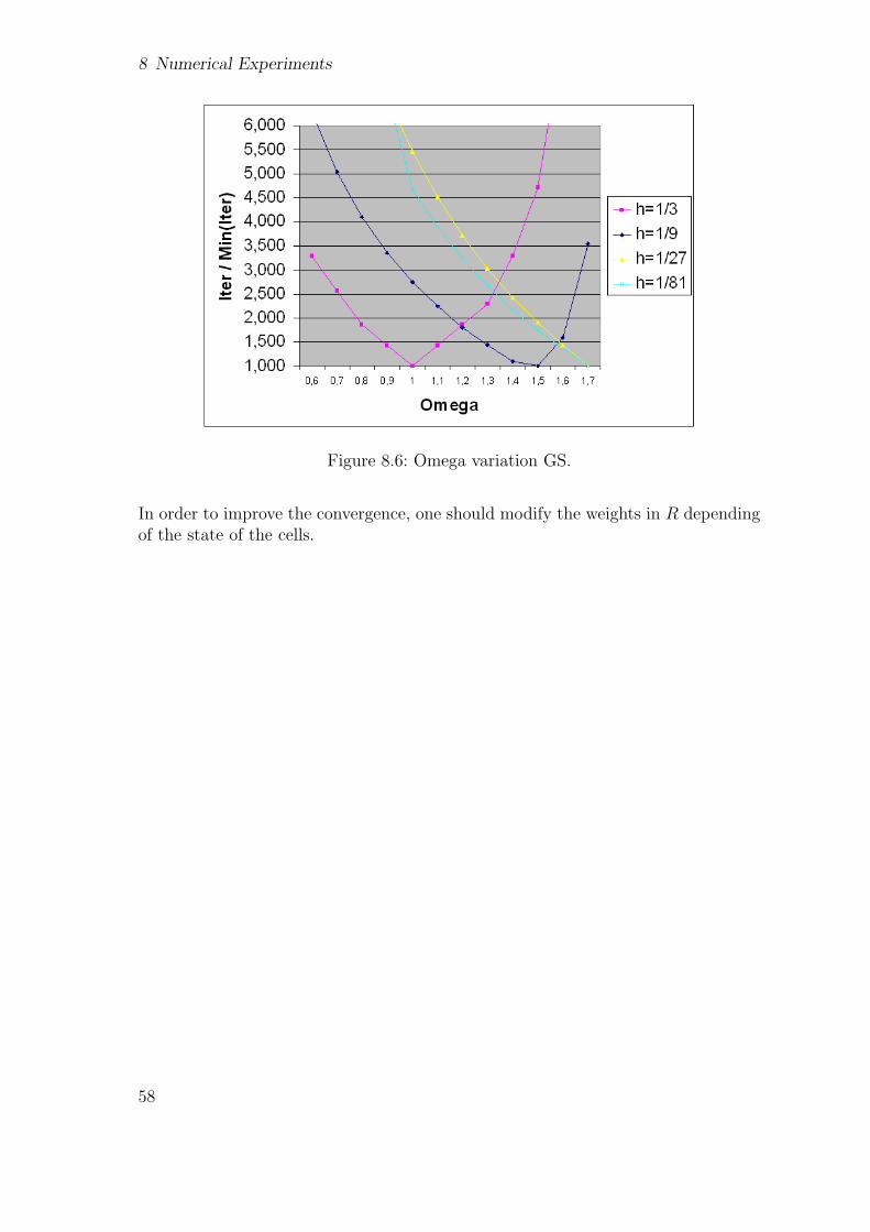
8 Numerical Experiments
Figure 8.6: Omega variation GS.
In order to improve the convergence, one should modify the weights in R dependingof the state of the cells.
58

8.3 HT-MG Convergence Analysis
Figure 8.7: Development of the ‖r‖2 depending on the number of iterations. Theresidual norm is logarithmized.
59

8 Numerical Experiments
60

9 Conclusions
In this thesis, we present a geometric multigrid scheme for staggered, elliptic bound-ary value problems. This scheme works strictly element-wise without setting up anysystem matrix. Thus, it comes along with very low memory requirements and fitsinto the Peano framework.
It was well-known before how to implement such a scheme for an additive multigridsolver. We extend it to a multiplicative full approximation storage scheme and makethe extension to adaptive grids straightforward. The extension to adaptive gridsexceeded our schedule and is yet to be done, but in [14] it is shown that it is rathersimple, as we have an explicit solution representation on all grid levels.
In CFD, inflow and outflow conditions correspond to Dirichlet boundary condi-tions in the pressure Poisson equation. In turn, solid walls imply Neumann condi-tions. As we implement both conditions, our solver is well-suited for the applicationwithin Peano’s CFD components. The integration is one of the first future steps.Furthermore, the numerical results exhibit that the treatment of the boundary cellsis critical: The stencils here have to be altered, as a naive treatment pollutes theconvergence rates. Our implementation offers the functionality to differ betweenboundary cells and inner cells. To implement the boundary stencils correctly wasbeyond our schedule. The underlying ideas and the solution is discussed in [11].
Standard multigrid theory relies on the Galerkin multigrid formulation. In thisthesis, we exploit the fact that full-weightening and a full stencil leads to exactlythe same stencil on each level. This does not hold for other stencils, i.e. thereis a need to store the prolongation and the restriction for these stencils in moredetails. Future work also has to examine the coarse grid operators for the domain’sboundary: As the stencil has to be altered at the boundary cell, the coarse gridoperator changes, too, according to the Galerkin multigrid formulation. This is alsopart of future work.
The extension of the solver to the three-dimensional case is outstanding. Theformalism within this thesis allows for a straightforward formulation of the three-dimensional operators. The mapping of the traversal to the algorithmic steps re-mains unaltered. Yet, implementing the three-dimensional operators brings alonglots of additional technical details and is not a trivial task.
Finally, we study the solver’s behavior for artificial small Poisson problems on veryregular computational domains. After an integration into a real CFD solver, run-time experiments for complicated scenarios will reveal whether the solver is able tocompete with other CFD codes. The preliminary results in this thesis are promising.
61

9 Conclusions
62
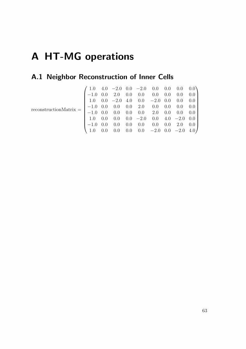
A HT-MG operations
A.1 Neighbor Reconstruction of Inner Cells
reconstructionMatrix =
1.0 4.0 −2.0 0.0 −2.0 0.0 0.0 0.0 0.0−1.0 0.0 2.0 0.0 0.0 0.0 0.0 0.0 0.01.0 0.0 −2.0 4.0 0.0 −2.0 0.0 0.0 0.0−1.0 0.0 0.0 0.0 2.0 0.0 0.0 0.0 0.0−1.0 0.0 0.0 0.0 0.0 2.0 0.0 0.0 0.01.0 0.0 0.0 0.0 −2.0 0.0 4.0 −2.0 0.0−1.0 0.0 0.0 0.0 0.0 0.0 0.0 2.0 0.01.0 0.0 0.0 0.0 0.0 −2.0 0.0 −2.0 4.0
63

A HT-MG operations
A.2 Interpolation Values of Hierarchical Surplus
−0.5 0.0 0.0 0.0 0.0 0.0 0.0 0.0 0.0,−0.5 0.0 0.0 0.0 0.0 0.0 0.0 0.0 0.0,−0.5 0.0 0.0 0.0 0.0 0.0 0.0 0.0 0.0,0.0 0.0 0.0 0.0 0.0 0.0 0.0 0.0 0.0,−0.5 −0.5 0.0 0.0 0.0 0.0 0.0 0.0 0.0,0.0 −0.5 0.0 0.0 0.0 0.0 0.0 0.0 0.00.0 −0.5 0.0 0.0 0.0 0.0 0.0 0.0 0.0−0.5 0.0 0.0 0.0 0.0 0.0 0.0 0.0 0.00.0 −0.5 −0.5 0.0 0.0 0.0 0.0 0.0 0.00.0 0.0 −0.5 0.0 0.0 0.0 0.0 0.0 0.00.0 0.0 −0.5 0.0 0.0 0.0 0.0 0.0 0.00.0 −0.5 0.0 0.0 0.0 0.0 0.0 0.0 0.00.0 0.0 −0.5 0.0 0.0 0.0 0.0 0.0 0.00.0 0.0 0.0 0.0 0.0 0.0 0.0 0.0 0.00.0 0.0 0.0 0.0 0.0 0.0 0.0 0.0 0.00.0 0.0 −0.5 0.0 0.0 0.0 0.0 0.0 0.00.0 0.0 0.0 −0.5 0.0 0.0 0.0 0.0 0.0−0.5 0.0 0.0 −0.5 0.0 0.0 0.0 0.0 0.00.0 0.0 0.0 −0.5 0.0 0.0 0.0 0.0 0.0−0.5 0.0 0.0 0.0 0.0 0.0 0.0 0.0 0.00.0 0.0 0.0 0.0 0.0 −0.5 0.0 0.0 0.00.0 0.0 0.0 0.0 0.0 0.0 0.0 0.0 0.00.0 0.0 −0.5 0.0 0.0 0.0 0.0 0.0 0.00.0 0.0 0.0 0.0 0.0 −0.5 0.0 0.0 0.00.0 0.0 0.0 0.0 0.0 0.0 −0.5 0.0 0.00.0 0.0 0.0 −0.5 0.0 0.0 −0.5 0.0 0.00.0 0.0 0.0 0.0 0.0 0.0 −0.5 0.0 0.00.0 0.0 0.0 −0.5 0.0 0.0 0.0 0.0 0.00.0 0.0 0.0 0.0 0.0 0.0 0.0 0.0 −0.50.0 0.0 0.0 0.0 0.0 0.0 0.0 0.0 0.00.0 0.0 0.0 0.0 0.0 −0.5 0.0 0.0 0.00.0 0.0 0.0 0.0 0.0 0.0 0.0 0.0 −0.50.0 0.0 0.0 0.0 0.0 0.0 0.0 0.0 0.00.0 0.0 0.0 0.0 0.0 0.0 −0.5 0.0 0.00.0 0.0 0.0 0.0 0.0 0.0 0.0 0.0 0.00.0 0.0 0.0 0.0 0.0 0.0 −0.5 0.0 0.00.0 0.0 0.0 0.0 0.0 0.0 0.0 0.0 0.00.0 0.0 0.0 0.0 0.0 0.0 0.0 −0.5 0.00.0 0.0 0.0 0.0 0.0 0.0 −0.5 0.0 0.00.0 0.0 0.0 0.0 0.0 0.0 0.0 −0.5 0.00.0 0.0 0.0 0.0 0.0 0.0 0.0 0.0 0.00.0 0.0 0.0 0.0 0.0 0.0 0.0 0.0 −0.50.0 0.0 0.0 0.0 0.0 0.0 0.0 −0.5 0.00.0 0.0 0.0 0.0 0.0 0.0 0.0 0.0 −0.50.0 0.0 0.0 0.0 0.0 0.0 0.0 0.0 0.00.0 0.0 0.0 0.0 0.0 0.0 0.0 0.0 0.00.0 0.0 0.0 0.0 0.0 0.0 0.0 0.0 −0.50.0 0.0 0.0 0.0 0.0 0.0 0.0 0.0 0.0
64

Bibliography
[1] William L. Briggs, Van Emden Henson, and Steve F. McCormick. A MultigridTutorial. SIAM, Heidelberg, Berlin, second edition, 2000.
[2] Hans-Joachim Bungartz, Wolfgang Eckhardt, Miriam Mehl, and TobiasWeinzierl. Dastgen - a data structure generator for parallel c++ hpc software.In Bubak, van Albada, Sloot, and Dongarra, editors, ICCS 2008: AdvancingScience through Computation, Part III, volume 5103 of Lecture Notes in Com-puter Science, pages 213–222, Heidelberg, Berlin, June 2008. Springer-Verlag.
[3] Hans-Joachim Bungartz, Miriam Mehl, and Tobias Weinzierl. A parallel adap-tive cartesian pde solver using space–filling curves. In E. Wolfgang Nagel,V. Wolfgang Walter, and Wolfgang Lehner, editors, Euro-Par 2006, ParallelProcessing, 12th International Euro-Par Conference, volume 4128 of LNCS,pages 1064–1074, Berlin Heidelberg, 2006. Springer-Verlag.
[4] Clive A. J. Fletcher. Computational Techniques for Fluid Dynamics. Compu-tational Physics. Heidelberg, Berlin, New York, second edition.
[5] Anton Frank. Organisationsprinzipien zur Integration von geometrischer Mod-ellierung, numerischer Simulation und Visualisierung. Dissertation, Munchen,2000.
[6] Michael Griebel. Zur Losung von Finite-Differenzen- und Finite-Element-Gleichungen mittels der Hiearchischen-Transformations-Mehrgitter-Methode.Dissertation, TU Munchen, February 1990.
[7] Michael Griebel. Multilevelmethoden als Iterationsverfahren uber Erzeugenden-systemen. Habilitationsschrift, TU Munchen, Stuttgart, 1994.
[8] Michael Griebel, Thomas Dornseifer, and Tilman Neunhoeffer. Numerical Sim-ulation in Fluid Dynamics: A Practical Introduction. Siam Monographs onMathematical Modeling and Computation. SIAM, Philadelphia, 1997.
[9] Miriam Mehl, Tobias Weinzierl, and Christoph Zenger. A cache-oblivious self-adaptive full multigrid method. Numerical Linear Algebra with Applications,13(2-3):275–291, 2006.
[10] William Mitchell. A refinement-tree based partitioning method for dynamicload balancing with adaptively refined grids. 2000.
65

Bibliography
[11] Tobias Neckel. Einfache 2d-fluid-struktur-wechselwirkungen mit einer cache-optimalen finite-element-methode. Diplomarbeit, Fakultat fur Informatik,Technische Universitat Munchen, 2005.
[12] Alfio Quarteroni, Riccardo Sacco, and Fausto Saleri. Numerische Mathematik1. Springer-Verlag, Heidelberg, Berlin, New York, 2002.
[13] Alfio Quarteroni and Fausto Saleri. Wissenschaftliches Rechnen mit MATLAB.Springer-Verlag, Heidelberg, Berlin, 2006.
[14] Ulrich Rude. Mathematical and computational techniques for multilevel adaptivemethods. Habilitationsschrift, TU Munchen, Philadelphia, 1993.
[15] Hans Sagan. Space-Filling Curves. Springer-Verlag, New York, 1994.
[16] Tobias Weinzierl. Eine cache-optimale Implementierung eines Navier-StokesLosers unter besonderer Berucksichtigung physikalischer Erhaltungssatze.Diplomarbeit, Fakultat fur Informatik, Technische Universitat Munchen, 2005.
[17] Tobias Weinzierl. Dissertation, TU Munchen, to be published.
66