A full computation-relevant topological dynamics classification of elementary cellularautomataMartin Schüle and Ruedi Stoop

Citation: Chaos: An Interdisciplinary Journal of Nonlinear Science 22, 043143 (2012); doi: 10.1063/1.4771662 View online: http://dx.doi.org/10.1063/1.4771662 View Table of Contents: http://scitation.aip.org/content/aip/journal/chaos/22/4?ver=pdfcov Published by the AIP Publishing Articles you may be interested in Towards the Full Lyapunov Spectrum of Elementary Cellular Automata AIP Conf. Proc. 1389, 981 (2011); 10.1063/1.3637774 On the topological sensitivity of cellular automata Chaos 21, 023108 (2011); 10.1063/1.3535581 Chaos of elementary cellular automata rule 42 of Wolfram’s class II Chaos 19, 013140 (2009); 10.1063/1.3099610 Cellular Automata with Memory AIP Conf. Proc. 661, 153 (2003); 10.1063/1.1571304 A cryptosystem based on cellular automata Chaos 8, 819 (1998); 10.1063/1.166368

This article is copyrighted as indicated in the article. Reuse of AIP content is subject to the terms at: http://scitation.aip.org/termsconditions. Downloaded to IP:

79.169.242.107 On: Sun, 11 May 2014 23:20:48

A full computation-relevant topological dynamics classification ofelementary cellular automata

Martin Sch€ulea) and Ruedi StoopInstitute of Neuroinformatics, ETH and University of Zurich, 8057 Zurich, Switzerland

(Received 5 June 2012; accepted 28 November 2012; published online 20 December 2012)

Cellular automata are both computational and dynamical systems. We give a complete

classification of the dynamic behaviour of elementary cellular automata (ECA) in terms of

fundamental dynamic system notions such as sensitivity and chaoticity. The “complex” ECA

emerge to be sensitive, but not chaotic and not eventually weakly periodic. Based on this

classification, we conjecture that elementary cellular automata capable of carrying out complex

computations, such as needed for Turing-universality, are at the “edge of chaos.” VC 2012 AmericanInstitute of Physics. [http://dx.doi.org/10.1063/1.4771662]

In the rich classical history of the theory of computation,

models of computation were typically compared to the

Turing machine concept, which allows us to characterize

their computational power in great detail.1,2

If, however,

one would like to ascribe “computational” capacity to

processes and systems observed in nature, one is naturally

pushed toward using dynamical systems notions as the nat-

ural framework, leaving the problem open of how to fit

this approach into, or how to link this approach with,

Turing computation. A paradigmatic class of systems that

comprise in a generic manner both computational and dy-

namical system aspects is the cellular automata (CA).

While CA are defined as a class of discrete dynamical sys-

tems, they also serve as a mathematical model of massively

parallel computation, a paradigm often observed when

“nature computes.” Remarkably, already very simple

rules make CA computationally universal, i.e., capable of

carrying out arbitrary computational tasks. By clarifying

the dynamical system properties of the most popular and

best-studied subclass of CA, the so-called elementary cellu-

lar automata (ECA), we will contribute here to a more

profound understanding of CA as both computational and

dynamical systems. We will fully classify the dynamic

behavior of ECA using exclusively topological dynamics

attributes such as sensitivity and chaos. Based on this clas-

sification, we will finally conjecture that the computation-

ally most complex and biologically relevant ECA are those

located at the “edge of chaos.”

I. INTRODUCTION

By definition, CA are discrete dynamical systems acting

in a discrete space-time. The state of a CA is specified by the

states of the individual cells of the CA, i.e., by the values

taken from a finite set of states associated with the sites of a

regular, uniform, infinite lattice. The state of a CA then

evolves in discrete time steps according to a rule acting syn-

chronously on the states in a finite neighbourhood of each

cell. Despite the simplicity of these rules, CA can exhibit

strikingly complex dynamical behaviour. A well-known

example of a CA with intricate dynamics is the so-called

Game of Life. CA have also been extensively applied as

models for a wide variety of physical and biological

processes.

Obtaining a dynamical system classification of ECA is

part of the long-standing problem in CA theory to character-

ise the “complexity” seen inherent in CA behaviour. In a se-

ries of influential papers, Wolfram studied the dynamical

system and statistical properties of CA and devised a classifi-

cation scheme.4–6 According to this scheme, CA behaviour

can be divided into the following classes:

(W1) almost all initial configurations lead to the same fixed

point configuration,

(W2) almost all initial configurations lead to a periodic

configuration,

(W3) almost all initial configurations lead to random looking

behaviour,

(W4) localized structures with complex behaviour emerge.

Wolfram’s classification attempt was largely based on

simulations of ECA. Since his pioneering work many more

classification schemes have been proposed, e.g., by Li et al.7

or Culik et al.8 It is however still an open problem of CA

theory to obtain a completely satisfying, formal classification

of CA behaviour.

In this paper, we will put forward a complete topological

dynamics classification of ECA. Our approach is based on

the symbolic dynamics treatment of CA initiated by the sem-

inal paper of Hedlund.3 The topological dynamics approach

allows to use the fundamental notions of dynamics system

theory such as sensitivity, chaos, etc. More specifically, the

classification is based on a scheme, introduced by Gilman9

and modified by Kurka,10 which proposes four classes: Equi-

continuous CA, CA with some equicontinuous points, sensi-

tive but not positively expansive CA, and positively

expansive CA. Each one-dimensional CA belongs to exactly

one class, but class membership is generally not decidable.10

We determine for every ECA, as far as we know for the first

time, to which class it belongs. We also (re-)derive further

properties such as surjectivity and chaoticity of ECA. Takena)schuelem@ini.phys.ethz.ch.

1054-1500/2012/22(4)/043143/10/$30.00 VC 2012 American Institute of Physics22, 043143-1

CHAOS 22, 043143 (2012)

This article is copyrighted as indicated in the article. Reuse of AIP content is subject to the terms at: http://scitation.aip.org/termsconditions. Downloaded to IP:

79.169.242.107 On: Sun, 11 May 2014 23:20:48

together, this gives a fairly complete picture of the dynami-

cal system properties of ECA.

The paper is organised as follows. In Sec. II, we intro-

duce one-dimensional CA and ECA formally. In Sec. III, we

give basic notations and definitions of the topological dy-

namics approach to CA. In Sec. IV, we introduce a scheme

that allows to express ECA rules algebraically. This will

prove helpful in Secs. V and VI, where we will classify ECA

in the topologically dynamics sense of Kurka. In Sec. VII,

we discuss our results.

II. DEFINITION OF ELEMENTARY CELLULARAUTOMATA

We start with the definitions of the basic concepts under-

lying the theory of one-dimensional CA. The configurationof a one-dimensional CA is given by the double-infinite

sequence x ¼ ðxiÞi2Z with xi 2 S being elements of the finite

set of states S ¼ f0; 1;…g. The configuration space X is the

set of all sequences x, i.e., X ¼ SZ. The CA map F, simply

called the CA F, is a map F : X! X where the local func-tion is the map f : S2rþ1 ! S; r � 1, with FðxÞi ¼ f ðxi�r;…; xi;…; xiþrÞ. The integer r is called the radius of the CA.

The iteration of the map F acting on an initial configuration

x generates the orbit x;FðxÞ;F2ðxÞ;… of x. The orbits of all

configurations x are a discrete space-time dynamical system

also referred to as CA F. Instances of the system can be

visualised in so-called space-time patterns.

A spatially periodic configuration is a configuration

which is invariant under translation in space, that is, x is peri-

odic if there is q > 1 such that rqðxÞ ¼ x where r : X! X is

the shift map rðxÞi ¼ xiþ1. A temporally periodic or simply

periodic configuration x for some CA F is given if FnðxÞ ¼ xfor some n > 0. If F(x)¼ x, x is called a fixed point. A con-

figuration x is called eventually periodic, if it evolves into a

temporally periodic configuration, i.e., if FkþnðxÞ ¼ FkðxÞfor some k � 0 and n > 0. If this holds for any configuration

x, the corresponding CA is called eventually periodic.

An ECA is an one-dimensional CA with two states and

“nearest neighbourhood coupling,” that is, S ¼ f0; 1g and

r¼ 1. There are then 256 different possible local functions

f : S3 ! S with FðxÞi ¼ f ðxi�1; xi; xiþ1Þ. Local functions are

also called rules and usually given in form of a rule table.

An example is

111 110 101 100 011 010 001 000

0 1 1 0 1 1 1 0

Every ECA rule is, following Wolfram,4 referred to by the

sequence of the values of the local function, as given in the

rule table, written as a decimal number. In the example

above, one speaks of ECA rule 110, because 01101110 writ-

ten as a decimal number equals 110.

III. TOPOLOGICAL AND SYMBOLIC DYNAMICSDEFINITIONS AND CONCEPTS

The framework we use to study the dynamical properties

of ECA is given by the symbolic dynamics approach that

views the state space SZ of one-dimensional CA as the

Cantor space of symbolic sequences. The topology of the

Cantor space is induced by the metric

dCðx; yÞ ¼Xþ1

i¼�1

dðxi; yiÞ2jij

;

where dðxi; yiÞ is the discrete metric

dðxi; yiÞ ¼1; xi 6¼ yi

0; xi ¼ yi:

�

Under this metric, the configuration space SZ is compact,

perfect, and totally disconnected, i.e., a Cantor space.11

From now on, the configuration space SZ endowed with this

metric will be referred to as X. The ECA functions F are con-

tinuous in X, hence (X, F) is a (discrete) dynamical system.

Now we introduce some key concepts of the topological

dynamics treatment of CA. A configuration x is an equiconti-nuity point of CA F, if 8� > 0; 9d > 0; 8y 2 X :

dðx; yÞ < d; 8n � 0 : dðFnðxÞ;FnðyÞÞ < �: (1)

If all configurations x 2 X are equicontinuity points then the

CA is called equicontinuous. If there is at least one equicon-

tinuity point, the CA is almost equicontinuous.

A CA is sensitive (to initial conditions), if

9� > 0; 8x 2 X; 8d > 0; 9y 2 X :

dðx; yÞ < d; 9n � 0 : dðFnðxÞ;FnðyÞÞ � �: (2)

A CA is positively expansive, if

9� > 0; 8x 6¼ y 2 X; 9n � 0 : dðFnðxÞ;FnðyÞÞ � �: (3)

Positively expansive CA are sensitive.11

If a configuration is an equicontinuity point, its orbit

remains arbitrarily close to the orbits of all sufficiently close

configurations. If a CA is sensitive, there exists for every con-

figuration at least one configuration arbitrarily close to it such

that the orbits of the two configurations will eventually be sep-

arated by some constant. Positive expansivity is a stronger

form of sensitivity: the orbits of all configurations that differ

in some cell will eventually be separated by some constant.

The long term behaviour of a sensitive CA can thus only be

predicted if the initial configuration is known precisely.

With these concepts, CA as dynamical systems can be

classified according to a classification introduced by Gilman9

and modified by Kurka.10 Every one-dimensional CA falls

exactly in one of the following classes:10

(K1) Equicontinuous CA.

(K2) Almost equicontinuous but not equicontinuous CA.

(K3) Sensitive but not positively expansive CA.

(K4) Positively expansive CA.

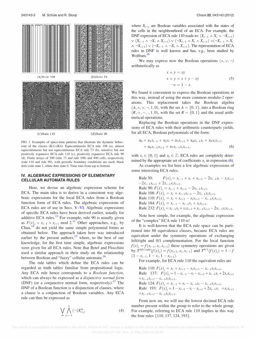
The typical emergent dynamics of the different classes

are illustrated by the space-time patterns of Figure 1.

It has been shown that for one-dimensional CA, it is not

decidable whether a given CA belongs to class (K1), (K2),

or ðK3Þ [ ðK4Þ, whereas it is still open whether the class

(K4) is decidable.12 We will show that it can be determined

to which class an ECA belongs.

043143-2 M. Sch€ule and R. Stoop Chaos 22, 043143 (2012)

This article is copyrighted as indicated in the article. Reuse of AIP content is subject to the terms at: http://scitation.aip.org/termsconditions. Downloaded to IP:

79.169.242.107 On: Sun, 11 May 2014 23:20:48

IV. ALGEBRAIC EXPRESSIONS OF ELEMENTARYCELLULAR AUTOMATA RULES

Here, we devise an algebraic expression scheme for

ECA. The main idea is to derive in a consistent way alge-

braic expressions for the local ECA rules from a Boolean

function form of ECA rules. The algebraic expressions of

ECA rules are of use in Secs. V–VI. Algebraic expressions

of specific ECA rules have been derived earlier, usually for

additive ECA rules.13 For example, rule 90 is usually given

as FðxÞi ¼ xi�1 þ xiþ1 mod 2.11 Other approaches, e.g., by

Chua,14 do not yield the same simple polynomial forms as

obtained below. The approach taken here was introduced

earlier by the present authors,15 where, to the best of our

knowledge, for the first time simple, algebraic expressions

were given for all ECA rules. Note that Betel and Flocchini

used a similar approach in their study on the relationship

between Boolean and “fuzzy” cellular automata.16

The rule tables which define the ECA rules can be

regarded as truth tables familiar from propositional logic.

Any ECA rule hence corresponds to a Boolean function,

which can always be expressed as a disjunctive normal form(DNF) (or a conjunctive normal form, respectively).17 The

DNF of a Boolean function is a disjunction of clauses, where

a clause is a conjunction of Boolean variables. Any ECA

rule can thus be expressed as

_m

1̂

j¼�1

ð:ÞXmiþj (4)

where Xiþj are Boolean variables associated with the states of

the cells in the neighbourhood of an ECA. For example, the

DNF expression of ECA rule 110 reads to: ðXi�1 � Xi � :Xiþ1Þ� ðXi�1 � :Xi � Xiþ1Þ � ð:Xi�1 � Xi � Xiþ1Þ �ð:Xi�1 � Xi

� :Xiþ1Þ � ð:Xi�1 � :Xi � Xiþ1Þ. The representation of ECA

rules in DNF is well known and has, e.g., been studied by

Wolfram.18

We may express now the Boolean operations ð�;�;:Þarithmetically as

x � y ¼ xy

x � y ¼ xþ y� xy

:x ¼ 1� x:

(5)

We found it convenient to express the Boolean operations in

this way, instead of using the more common modulo-2 oper-

ations. This replacement takes the Boolean algebra

ðA;�;�;:; 1; 0Þ, with the set A ¼ f0; 1g, into a Boolean ring

ðR;þ;�; �; 1; 0Þ, with the set R ¼ f0; 1g and the usual arith-

metical operations.

Replacing the Boolean operations in the DNF expres-

sions of ECA rules with their arithmetic counterparts yields,

for all ECA, Boolean polynomials of the form:

a0 þ a1xi�1 þ a2xi þ a3xiþ1 þ a4xi�1xi þ a5xixiþ1

þ a6xi�1xiþ1 þ a7xi�1xixiþ1; (6)

with xi 2 f0; 1g and aj 2 Z. ECA rules are completely deter-

mined by the appropriate set of coefficients aj in expression (6).

As examples we list here a few algebraic expressions of

some interesting ECA rules.

Rule 30: FðxÞi¼ xi�1 þ xi þ xiþ1 � 2xi�1xi � xixiþ1

�2xi�1xiþ1 þ 2xi�1xixiþ1.

Rule 90: FðxÞi ¼ xi�1 þ xiþ1 � 2xi�1xiþ1.

Rule 108: FðxÞi ¼ xi þ xi�1xiþ1 � 2xi�1xixiþ1.

Rule 110: FðxÞi ¼ xi þ xiþ1 � xixiþ1 � xi�1xixiþ1.

Rule 184: FðxÞi ¼ xi�1 � xi�1xi þ xixiþ1.

Rule 232: FðxÞi¼ xi�1xiþxixiþ1þxi�1xiþ1�2xi�1xixiþ1.

Note how simple, for example, the algebraic expression

of the “complex” ECA rule 110 is!

It is well-known that the ECA rule space can be parti-

tioned into 88 equivalence classes, because ECA rules are

equivalent under the symmetry operations of exchanging

left/right and 0/1 complementation. For the local function

f ðxÞi ¼ f ðxi�1; xi; xiþ1Þ these symmetry operations are given

by Tleft=rightðf ðxÞiÞ ¼ f ðxiþ1; xi; xi�1Þ and T0=1ðf ðxÞiÞ ¼ 1� fð1� xi�1; 1� xi; 1� xiþ1Þ.

For example, for ECA rule 110 the equivalent rules are

Rule 110: FðxÞi ¼ xi þ xiþ1 � xixiþ1 � xi�1xixiþ1.

Rule 137: FðxÞi¼1�xi�1�xi�xiþ1þxi�1xiþ2xixiþ1

þxi�1xiþ1�xi�1xixiþ1.

Rule 124: FðxÞi ¼ xi�1 þ xi � xi�1xi � xi�1xixiþ1.

Rule 193: FðxÞi¼1�xi�1�xi�xiþ1þ2xi�1xi þxixiþ1

þxi�1xiþ1�xi�1xixiþ1.

From now on, we will use the lowest decimal ECA rule

number present within the group to refer to the whole group.

For example, referring to ECA rule 110 implies in this way

the four rules f110; 137; 124; 193g.

FIG. 1. Examples of space-time patterns that illustrate the dynamic behav-

iour of the classes (K1)-(K4): Equicontinuous ECA rule 108 (a), almost

equicontinuous but not equicontinuous ECA rule 73 (b), sensitive but not

positively expansive ECA rule 110 (c), positively expansive ECA rule 90

(d). Finite arrays of 200 (rule 73 and rule 108) and 400 cells, respectively

(rule 110 and rule 90), with periodic boundary conditions are used; black

dots code state 1, white dots state 0. Time runs from top to bottom.

043143-3 M. Sch€ule and R. Stoop Chaos 22, 043143 (2012)

This article is copyrighted as indicated in the article. Reuse of AIP content is subject to the terms at: http://scitation.aip.org/termsconditions. Downloaded to IP:

79.169.242.107 On: Sun, 11 May 2014 23:20:48

Note that the approach developed here can be extended

in various ways, for example to one-dimensional CA with

state space f0; 1g with larger neighbourhood, or to two-

dimensional CA with state space f0; 1g, etc.

V. CLASSIFICATION OF ELEMENTARY CELLULARAUTOMATA

We will now classify ECA from their topological dy-

namics properties, that is, according to the scheme intro-

duced by Gilman9 and modified by Kurka.10

First, we need some more symbolic dynamics definitions

and notions. A word u is a finite symbolic sequence

u ¼ u0…ul�1, with ui 2 S, where S is a finite alphabet, e.g.,

in the case of ECA the state set f0; 1g. The length of u is

denoted by l ¼ juj. The set of words of S of length l is

denoted by Sl, the set of all words of S with l > 0 is Sþ. The

cylinder set ½u�0 of u consists of all points x 2 SZ with lead-

ing part u, i.e., ½u�0 ¼ fx 2 SZ : x½0;lÞ ¼ ug.A word u 2 Sþ with juj � m;m > 0, is m-blocking for a

one-dimensional CA F, if there exists an offset q 2½0; juj � m� such that

8x; y 2 ½u�0; 8n � 0;FnðxÞ½q;qþmÞ ¼ FnðyÞ½q;qþmÞ:

For an illustration of the mathematical definition, see Figure 2.

One-dimensional CA, and therefore ECA, are either sen-

sitive or almost equicontinuous. The latter property is equiv-

alent to having a blocking word:

Proposition 1 (Kurka11). For any one-dimensional CA Fwith radius r > 0 the following conditions are equivalent.

(1) F is not sensitive.(2) F has an r-blocking word.(3) F is almost equicontinuous.

If a configuration x contains a m-blocking word u, then

the sequence x½q;qþmÞ, i.e., the states of the cells in the seg-

ment ½q; qþ mÞ, are at all times independent of the initial

states outside of the blocking word u. Hence, the following

corollary holds.

Corollary 2. For any one-dimensional CA F with radiusr > 0, the following conditions are equivalent.

(1) F has a m-blocking word with m � r.

(2) F has a word u 2 Sþ with juj � m;m > 0 and an offsetq 2 ½0; juj � m� such that 8x 2 ½u�0 the sequence x½q;qþmÞ iseventually temporally periodic.

Proof. ð1Þ ) ð2Þ: Denote the sequence x½q;qþmÞ of a block-

ing word u that is at all times independent of the initial states

outside of u by v. The configuration x ¼ ðuÞ1 is spatially peri-

odic and hence eventually temporally periodic. Because the

sequence v is independent of the states of the cells outside of u,

the sequence v is also eventually temporally periodic.

ð2Þ ) ð1Þ: The condition (2) says that for all x 2 ½u�0 there

is t � 0 and p > 0 such that FtþpðxÞ½q;qþmÞ ¼ FtðyÞ½q;qþmÞ.Thus, for all x; y 2 ½u�0 and all n � 0 the sequence

FnðxÞ½q;qþmÞ ¼ FnðyÞ½q;qþmÞ must be independent of the initial

states outside of u, hence the word u is m-blocking. (

We will now systematically search for blocking words.

We know by Proposition 1 that whenever a blocking word can

be found, the corresponding ECA is almost equicontinuous. By

Corollary 2, we know that this corresponds to finding a word uthat contains a sequence that is eventually temporally periodic,

independent of the initial states outside of u. As it turns out, we

can thereby effectively determine all almost equicontinuous

ECA, because any almost equicontinuous ECA corresponds to

a blocking word u for which the length l ¼ juj is bounded.

Proposition 3. Each almost equicontinuous ECA has atleast one blocking word of length l � 4.

Proof. In the following, we look for blocking words,

starting with the smallest possible length l¼ 1 and then suc-

cessively for words of greater length (for a visualisation of

the definition of a blocking word, see again Figure 2). If a

blocking word can be found, one or several almost equicon-

tinuous ECA rules will satisfy the blocking conditions. The

ECA rules are specified by a rule table which we denote by

ðt0; t1; t2; t3; t4; t5; t6; t7Þ. For example, ECA rule 110 is given

by the table (0, 1, 1, 0, 1, 1, 1, 0). If an entry in the rule table

is left unspecified, the entry can take on either of the two val-

ues 0 or 1, e.g., the table ð0; 1; 1; 0; 1; 1; 1; t7Þ refers to the

two ECA rules 110 and 111. If a blocking word can be

found, we put the ECA rule table admitted by the blocking

conditions in a list. A blocking word u and the admitted rule

table is denoted by tðu; pÞ ¼ ðt0; t1; t2; t3; t4; t5; t6; t7Þ, where

p is the period with which the eventually periodic sequence

in the word u (i.e., the sequence x½q;qþmÞ referred to in Corol-

lary 2) is repeated. For example, tð00; 1Þ ¼ ðt0; t1; t2; 0; t4;t5; 0; 0Þ refers to the blocking word 00 of period p¼ 1 that

corresponds to 25 ¼ 32 ECA rules, as denoted by the rule ta-

ble. If a newly found blocking word admits ECA rules gener-

ated by a rule table obtained by a blocking word already in

the list (hence of smaller length), the word and the rule table

admitted by it is not listed. We also do not list blocking

words, and the rule tables admitted by them, if they corre-

spond to ECA rules equivalent to ECA rules admitted by a

blocking word already in the list.

Let us further assume the following notation: The vari-

able ci always denotes the states of cells i of a blocking word

u that are at all times independent of the initial states of the

cells outside of the blocking word u. The variable xi on the

other hand denotes the states of cells i that are in principle

influenceable by the initial states of the cells outside of u.

The state xi of such a cell i is left undetermined, i.e., the

value can either be 0 or 1. If it is known for configurations

x; y 2 ½u�0 that the states xi and yi of some cell i differ, we

FIG. 2. A word u of length juj ¼ l is said to be blocking, if it has an interior

of size m, located from position q, that remains unaffected by the states of

the cells left and right to the word u, at all times.

043143-4 M. Sch€ule and R. Stoop Chaos 22, 043143 (2012)

This article is copyrighted as indicated in the article. Reuse of AIP content is subject to the terms at: http://scitation.aip.org/termsconditions. Downloaded to IP:

79.169.242.107 On: Sun, 11 May 2014 23:20:48

write �xi. For example, the “scenario”�x�1 c0 �x1

x�1 c0 x1refers to

two configurations x; y 2 ½u�0 that share the blocking word

u ¼ c0 of length l¼ 1 that is repeated with period p¼ 1. At

the boundaries of the blocking word u, here at the cells

i¼�1 and i¼ 1, we can assume that the configurations xand y differ, which is denoted by �x�i and �xi, whereas in the

next time step this may not necessarily be the case anymore

(at the cells i¼�1 and i¼ 1).

The proof has two parts. In part A, we determine all

blocking words of length l � 4. In part B, we show that for

any blocking word u of length l > 4 there is a corresponding

blocking word of length l � 4.

Part A: Let us look at the cases (a) l¼ 1, (b) l¼ 2, (c)

l¼ 3, and (d) l¼ 4, where l, as said, denotes the length of a

blocking word u.

(a) With l¼ 1, the following scenarios are possible: (1)

�x�1 c0 �x1

x�1 c0 x1, (2)

�x�1 c0 �x1

c0 c0 x1, (3)

�x�1 c0 �x1

x�1 c0 c0,

(4)�x�1 c0 �x1

c0 c0 c0, (5)

�x�1 c0 �x1

x�1 c00 x1, (6)

�x�1 c0 �x1

c0�1 c00 x1,

(7)�x�1 c0 �x1

x�1 c00 c01, and (8)

�x�1 c0 �x1

c0�1 c00 c01,where at least

for one i, c0i 6¼ ci. Note that there are further scenarios

possible that however do not yield further valid rule

tables and are not listed here. Scenario (1) yields the

rule table tð1; 1Þ ¼ ð1; 1; t2; t3; 1; 1; t6; t7Þ (and the table

tð0; 1Þ ¼ ðt0; t1; 0; 0; t4; t5; 0; 0Þ, but as said, tables that

yield ECA rules equivalent to already obtained rules

are not listed). Scenarios (2), (3), and (4) do not admit

rule tables that yield ECA rules not already listed. For

scenario (5), two cases have to be further distinguished:

�x�1 c0 �x1

x�1 c00 x1

c00

and

�x�1 c0 �x1

x�1 c00 x1

c0

, where c00 6¼ c0. The

first case does not lead to new ECA rules. The second

case yields the rule table t(1, 2)¼ (0, 0, 1, 1, 0, 0, 1, 1).

Scenarios (6) and (7) yield rule tables already listed.

Scenario (8) yields t(1, 2)¼ (0, 0, 0, 0, 0, 0, 0, 1).

(b) For l¼ 2, we deal with essentially the same scenarios

as in case (a). For example, in analogy to the scenario

(1)�x�1 c0 �x1

x�1 c0 x1of case (a), we have the scenario

�x�1 c0 c1 �x2

x�1 c0 c1 x2. However, for reasons of space, we

cannot list all possible scenarios and from now on only

list the scenarios that yield blocking words that admit

rule tables not yet obtained. These are: (1)

�x�1 c0 c1 �x2

x�1 c0 c1 x2and (2)

�x�1 c0 c1 �x2

x�1 c00 c01 x2, where

c0i 6¼ ci. Scenarios (1) and (2) yield, as can easily be

checked, the following blocking words and rule tables:

tð00; 1Þ ¼ ðt0; t1; t2; 0; t4; t5; 0; 0Þ; tð01; 1Þ ¼ ðt0; t1; 0; t3;1; 1; 0; t7Þ; tð10; 1Þ ¼ ðt0; 1; 0; 0; t4; 1; t6; t7Þ and

tð00; 2Þ ¼ ð0; 0; t2; 1; 0; t5; 1; 1Þ; tð10; 2Þ ¼ ðt0; 0; 1; 1;0; 0; 1; t7Þ.

(c) For l¼ 3, the scenarios that yield rule tables not listed

above are: (1)�x�1 c0 c1 c2 �x3

x�1 c0 c1 c2 x3and (2)

�x�1 c0 c1 c2 �x3

x�1 �x0 c01 �x2 x3

c0 c1 c2

, where c01 6¼ c1. Scenario (1)

yields the blocking words and rule tables tð010; 1Þ ¼ðt0; t1; 0; 0; t4; 1; 0; t7Þ and tð101; 1Þ ¼ ðt0; 1; 0; t3; 1; 1;t6; t7Þ. Scenario (2) yields tð000; 2Þ ¼ ð0; 0; t2; 0; 0; 0;0; 1Þ. Note that for example the scenario

�x�1 c0 c1 c2 �x3

x�1 �x0 c1 �x2 x3

c0 c1 c2

does not yield new rule tables.

(d) For l¼ 4, the only scenario that leads to a blocking

word corresponding to a rule table not yet listed is

�x�1 c0 c1 c2 c3 �x4

x�1 c0 c1 c2 c3 x4, yielding the rule table

tð0110; 1Þ ¼ ðt0; 1; 0; 0; 1; t5; 0; t7Þ. Note again that,

e.g., the scenario

�x�1 c0 c1 c2 c3 �x4

x�1 �x0 c01 c02 �x3 x4

c0 c1 c2 c3

, where at

least for one i c0i 6¼ ci, does not yield new rule tables.

With this we conclude Part A. Let us list the blocking

words and the rule tables admitted by them that we

have found so far

tð0; 1Þ ¼ ðt0; t1; 0; 0; t4; t5; 0; 0Þt(1, 2)¼ (0, 0, 1, 1, 0, 0, 1, 1)

t(1, 2)¼ (0, 0, 0, 0, 0, 0, 0, 1)

tð00; 1Þ ¼ ðt0; t1; t2; 0; t4; t5; 0; 0Þtð01; 1Þ ¼ ðt0; t1; 0; t3; 1; 1; 0; t7Þtð10; 1Þ ¼ ðt0; 1; 0; 0; t4; 1; t6; t7Þtð00; 2Þ ¼ ð0; 0; t2; 1; 0; t5; 1; 1Þtð01; 2Þ ¼ ðt0; 0; 1; 1; 0; 0; 1; t7Þ

tð010; 1Þ ¼ ðt0; t1; 0; 0; t4; 1; 0; t7Þtð101; 1Þ ¼ ðt0; 1; 0; t3; 1; 1; t6; t7Þtð000; 2Þ ¼ ð0; 0; t2; 0; 0; 0; 0; 1Þ

tð0110; 1Þ ¼ ðt0; 1; 0; 0; 1; t5; 0; t7Þ

Part B: In the general case, i.e., for l > 4, we can con-

clude in analogy to the cases already considered, i.e., the

cases with l � 4, that the following scenarios could possibly

lead to new blocking words:

(1)�x�1 c0 c1 … cl�2 cl�1 �xl

x�1 c0 c1 … cl�2 cl�1 xl

� �;

(2)�x�1 c0 c1 … cl�2 cl�1 �xl

c�1 c0 c1 … cl�2 cl�1 cl

� �;

(3)

�x�1 c0 c1 … … cl�2 cl�1 �xl

…

�xq�1 cq … cqþm�1 �xqþm

xq�1 cq … cqþm�1 xqþm

0BB@

1CCA;

(4)

�x�1 c0 c1 … … cl�2 cl�1 �xl

…

�xq�1 cq … cqþm�1 �xqþm

cq�1 cq … cqþm�1 cqþm

0BB@

1CCA;

(5)�x�1 c0 c1 … cl�2 cl�1 �xl

x�1 c00 c01 … c0l�2 c0l�1 xl

� �;

(6)�x�1 c0 c1 … cl�2 cl�1 �xl

c0�1 c00 c01 … c0l�2 c0l�1 c0l

� �;

043143-5 M. Sch€ule and R. Stoop Chaos 22, 043143 (2012)

This article is copyrighted as indicated in the article. Reuse of AIP content is subject to the terms at: http://scitation.aip.org/termsconditions. Downloaded to IP:

79.169.242.107 On: Sun, 11 May 2014 23:20:48

(7)

�x�1 c0 c1 … … cl�2 cl�1 �xl

…

�xq�1 cq … cqþm�1 �xqþm

xq�1 c0q … c0qþm�1 xqþm

0BB@

1CCA;

(8)

�x�1 c0 c1 … … cl�2 cl�1 �xl

…

�xq�1 cq cqþ1 … cqþm�2 cqþm�1 �xqþm

�xq c0qþ1 … c0qþm�2 �xqþm�1

cq cqþ1 … cqþm�2 cqþm�1

0BBBB@

1CCCCA;

with m � 1 and where at least for one i, c0i 6¼ ci.

Case (1) yields blocking words already listed, because for

l > 4 the conditions to be satisfied in order to obtain a block-

ing word u are entailed in the conditions to obtain a blocking

word u with l � 4. The same reasoning applies to cases (2),

(3), and (4). The basic reason that such a reduction is possible

is due to the fact that the conditions to be satisfied in order to

obtain a blocking word depend on the values of the boundary

cells, here the values �x�1 and �xl (respectively, the values �xq�1

and �xqþm in cases (3) and (4)), but not on the values of the

cells to the left (of i¼ –1) and right (of i¼ l) of the boundary

cells, as can be checked with the scenarios treated in Part A.

Let us then look closer at case (5). We will show that if

there is a blocking word c1c2…cl�2cl�1, the word is repeated

with period p¼ 2, because if the word is blocking, the word at

the next time step (in case (5)) must be �c1�c2…�cl�2�cl�1. The

bar signifies that the state ci of the cell i must change, i.e.,

�ci ¼ ð1� ciÞ. Without loss of generality, we can consider

only the 24 boundary conditions for blocking words at succes-

sive time steps. That is, given the word c1c2…cl�2cl�1, we

consider at the next time-step all the ð24 � 2Þ possible cases:

c1c2…cl�2�cl�1; c1c2…�cl�2cl�1, etc., excluding the two cases

c1c2…cl�2cl�1 and �c1�c2…�cl�2�cl�1. It suffices to consider the

case c1c2…cl�2�cl�1. The other cases can be dealt with analo-

gously. The temporal evolution of the ECA generates in this

case the following scheme:

�x�1 c0 c1 … cl�2 cl�1 �xl

x�1 c0 c1 … cl�2 �cl�1 xl

x�1 c0 c1 … �cl�2 c2l�1 xl

…

x�1 c0 �c1 … cl�2l�2 cl�2

l�1 xl

x�1 �c0 cl�11 … cl�1

l�2 cl�1l�1 xl

The superscript denotes the time-step n. The third, fifth, and

sixth line are due to the fact that if the state of, e.g., the cell

l – 2 at time step n¼ 2 did not change, one would obtain a

blocking word of shorter length (l – 1). By checking all 24

possible values for the boundary states of the initial word

c1c2…cl�2cl�1 it can be shown that the above scheme cannot

be satisfied. Thus, any initial word c1c2…cl�2cl�1 evolves in

the next time step into either the word c1c2…cl�2cl�1 or the

word �c1�c2…�cl�2�cl�1. In the first case, a blocking word of pe-

riod p¼ 1 is found, in the second case, i.e., for p¼ 2, one can

find a blocking word of length l¼ 2, as can easily be shown.

The case (6) can be reduced to the case already treated

under (a (8)) in Part A, the case (7) to the case (5) and the

case (8) again to the case treated under (c (2)) (or the exam-

ple in (d), respectively) in Part A.

With this we conclude our analysis. In Part A, we have

identified all blocking words of length l � 4. For l � 2, we

omitted, for reasons of space, the presentation of the cases

that do not lead to blocking words or to blocking words al-

ready identified. In Part B, we have concluded from the cases

for l � 4 on the general form of the scenarios that could pos-

sibly lead to blocking words for l > 4. These general scenar-

ios could then be reduced to the scenarios obtained for l � 4.

One case (case (5)) required a separate treatment and was

analysed by means of an example.

To arrive at a complete list of blocking words for l � 4

and to exclude additional blocking words for l > 4, great

care and efforts have been invested. We have tested the

completeness of the list also by extensively sampling the

space of initial configurations for ECA, which yielded no

additional blocking words. One may also check the correct-

ness and completeness of the cases investigated in our anal-

ysis by hand with the help of a computer, running a

program that follows the lines of the proof above. Alterna-

tively, to demonstrate the impossibility of additional block-

ing words, the systems of equations generated from the

conditions for blocking words and the algebraic expressions

of ECA rules could be used, systematically evaluated for

each single case. �

The proof of Proposition 3 allows to give, for ECA, a

stronger version of Proposition 1. Let us call a word u of

length l invariant for an ECA F, if for all x 2 ½u�0, there is a

p > 0 such that FpðxÞ½0;lÞ ¼ x½0;lÞ.Corollary 4. An ECA F is almost equicontinuous if and

only if F has an invariant word.Proof. See the proof of Proposition 3. �

Proposition 3 (or Corollary 4, respectively) allows us to

determine for each ECA rule whether it is almost equicontin-

uous or not. It is almost equicontinous if there is an associ-

ated blocking word on the list composed of the invariant

words of shortest length. Below, we provide this list together

with the corresponding almost equicontinuous ECA rules.

Corollary 5. Invariant words of period p¼ 1 and corre-sponding ECA rules:

0: 0, 4, 8, 12, 72, 76, 128, 132, 136, 140, 200, 204.00: 32, 36, 40, 44, 104, 108, 160, 164, 168, 172, 232.01: 13, 28, 29, 77, 156.10: 78.010: 5.101: 94.0110: 73.Invariant words of period p¼ 2 and corresponding ECA

rules:1: 1.0: 51.00: 19, 23.01: 50, 178.000: 33.Conversely, we now also know the sensitive ECA rules.

Proposition 6. The following rules are sensitive:2, 3, 6, 7, 9, 10, 11, 14, 15, 18, 22, 24, 25, 26, 27, 30, 34,

35, 37, 38, 41, 42, 43, 45, 46, 54, 56, 57, 58, 60, 62, 74, 90,105, 106, 110, 122, 126, 130, 134, 138, 142, 146, 150, 152,154, 162, 170, 184.

043143-6 M. Sch€ule and R. Stoop Chaos 22, 043143 (2012)

This article is copyrighted as indicated in the article. Reuse of AIP content is subject to the terms at: http://scitation.aip.org/termsconditions. Downloaded to IP:

79.169.242.107 On: Sun, 11 May 2014 23:20:48

Proof. Follows from Propositions 1, 3, and Corollary 5. �

The class of sensitive ECA is large, because in the Can-

tor space left- or right-shifting rules are sensitive. We will

later return to this point.

From the almost equicontinuous ECA rules, we can fur-

ther specify the equicontinuous ones. We use the following

lemma.

Lemma 7 (Kurka11). A one-dimensional almost equicon-tinuous CA F is equicontinuous if and only if:

(1) There exists a preperiod m � 0 and a period p > 0,such that Fmþp ¼ Fm.

It is almost equicontinuous but not equicontinuous if andonly if:

(2) There is at least one point x 2 X for which the almostequicontinuous CA F is not equicontinuous.

Proposition 8. The following rules are equicontinuous:0, 1, 4, 5, 8, 12, 19, 29, 36, 51, 72, 76, 108, 200, 204.Proof. The proof is by showing that condition (1) of Lemma

7 holds. We only give an example for a specific ECA rule.

Rule 72 is equicontinuous with preperiod m¼ 2 and pe-

riod p¼ 1, because, by using the algebraic expression for the

local function, we obtain

FðxÞi ¼ xi�1xi þ xixiþ1 � 2xi�1xixiþ1;

F2ðxÞi ¼ xi�1xi � xi�2xi�1xi þ xixiþ1 � 2xi�1xixiþ1

þ xi�2xi�1xixiþ1 � xixiþ1xiþ2 þ xi�1xixiþ1xiþ2;

F3ðxÞi ¼ xi�1xi � xi�2xi�1xi þ xixiþ1 � 2xi�1xixiþ1

þ xi�2xi�1xixiþ1 � xixiþ1xiþ2 þ xi�1xixiþ1xiþ2:

Hence, F3ðxÞi ¼ F2ðxÞi; 8i 2 Z. Thus, F3 ¼ F2. �

Proposition 9. The following rules are almost equicon-tinuous but not equicontinuous:

13, 23, 28, 32, 33, 40, 44, 50, 73, 77, 78, 94, 104, 128,132, 136, 140, 156, 160, 164, 168, 172, 178, 232.

Proof. The proof is by showing that condition (2) of Lemma

7 holds. We only give an example for a specific ECA rule.

ECA rule 104 is almost equicontinuous but not equicon-

tinuous, because ð10Þ1 is not an equicontinuous point.

Assume the configuration x ¼ ð10Þ1 and an integer q >0 such that

8y 2 X; ðx½�q;q� ¼ y½�q;q�Þ ) ðdðx; yÞ < 2�qÞ:

Assume that y differs from x at cells (– q – 1) and (qþ 1), that is,

y�q�1 ¼ 1� x�q�1 and yqþ1 ¼ 1� xqþ1. Then, as can easily

be shown by using the algebraic expression of ECA rule 104,

dðFnðxÞ;FnðyÞÞ > 2�ðq�nÞ;

for all n � q. Hence, ECA 104 is not equicontinuous at the

point x ¼ ð10Þ1. �

From the sensitive ECA, we can distinguish further the

positively expansive ECA.

First, we need the definition of permutivity for ECA.19

An ECA F is left-permutive if ð8u 2 S2Þ; ð8b 2 SÞ;ð9!a 2 SÞ: f(au)¼ b. It is right-permutive if ð8u 2 S2Þ; ð8b 2SÞ; ð9!a 2 SÞ: f(ua)¼ b. The ECA F is permutive if it is ei-

ther left-permutive or right-permutive.

We will use the following lemma:

Lemma 10 (Kurka11). A one-dimensional CA F is posi-tively expansive if the following condition holds.

(1) The CA is both left- and right-permutive.A one-dimensional sensitive CA F is not positively expansiveif and only if the following condition holds.

(2) There is no � > 0 such that for all x 6¼ y 2 X there isn � 0 with dðFnðxÞ;FnðyÞÞ � �.

Proposition 11. The following ECA rules are sensitivebut not positively expansive:

2, 3, 6, 7, 9, 10, 11, 14, 15, 18, 22, 24, 25, 26, 27, 30, 34, 35,37, 38, 41, 42, 43, 45, 46, 54, 56, 57, 58, 60, 62, 74, 106, 110,122, 126, 130, 134, 138, 142, 146, 152, 154, 162, 170, 184.

Proof. The proof is by showing that condition (2) of

Lemma 10 holds. We only provide the example of a specific

ECA rule.

ECA rule 110 is sensitive but not positively expansive.

Assume the expansivity constant � ¼ 2�m, then

8x 6¼ y 2 X) 9n � 0;FnðxÞ½�m;m� 6¼ FnðyÞ½�m;m� (7)

must hold. Assume the configuration x ¼ ð00110111110001Þ1and an integer q > 0 such that 14q > m. Then, for a configura-

tion y 2 X that differs from x at the cells 14q, 14q þ 1, 14q þ 2,

Eq. (7) does not hold. �

Proposition 12. The following ECA rules are positivelyexpansive:

90, 105, 150.Proof. For ECA rules 90, 105 and 150 condition (1) of

Lemma 10 holds. �

For ECA left- and right-permutivity is equivalent to pos-

itive expansivity.

Proposition 13. ECA are positively expansive if andonly if they are both left- and right-permutive.

Proof. Follows from Propositions 6, 11, and 12. �

Note that Proposition 13 does not hold generally for

one-dimensional CA.11

We summarize the findings of this section in Table I,

which shows all ECA rules according to whether they have

the property of equicontinuity, almost equicontinuity, sensi-

tivity or positively expansivity.

TABLE I. Topological dynamics classification of ECA rules.

Almost equicontinuous Sensitive

Equicontinuous Positively expansive

0, 1, 4, 5, 8, 13, 23, 28, 32, 2, 3, 6, 7, 9, 90, 105, 150

12, 19, 29, 36, 33, 40, 44, 50, 73, 10, 11, 14, 15,

51, 72, 76, 108, 77, 78, 94, 104, 18, 22, 24, 25,

200, 204 128, 132, 136, 140, 26, 27, 30, 34,

156, 160, 164, 168, 35, 37, 38, 41,

172, 178, 232 42, 43, 45, 46,

54, 56, 57, 58,

60, 62, 74, 106,

110, 122, 126, 130,

134, 138, 142, 146,

152, 154, 162,

170, 184

043143-7 M. Sch€ule and R. Stoop Chaos 22, 043143 (2012)

This article is copyrighted as indicated in the article. Reuse of AIP content is subject to the terms at: http://scitation.aip.org/termsconditions. Downloaded to IP:

79.169.242.107 On: Sun, 11 May 2014 23:20:48

VI. CLASSIFICATION OF SENSITIVE ELEMENTARYCELLULAR AUTOMATA

Since the beginning of CA research, the classification of

the degree of “complexity” seen in CA behaviour has been a

main research focus. It is intuitively clear that the sensitivity

property is a source of the apparent “complexity” of ECA

behaviour. Among the sensitive ECA rules, we find, however,

rules that show in their space-time dynamics “travelling waves”

patterns (Fig. 3). These non-complex shift-dynamics patterns

are from eventually weakly periodic ECA defined as follows.

A configuration x is called weakly periodic, if there is q 2Z and p > 0 such that FprqðxÞ ¼ x.19 We define a configura-

tion x as eventually weakly periodic if there is q 2 Z and

n; p > 0 such that FnþprqðxÞ ¼ FnðxÞ. We call an ECA even-tually weakly periodic, if the ECA is not eventually periodic,

but for all configurations x eventually weakly periodic.

Proposition 14. The following sensitive ECA rules areeventually weakly periodic:

2, 3, 10, 15, 24, 34, 38, 42, 46, 138, 170.Proof. The general proof follows the argument exhibited

for a specific ECA rule as follows.

Employing the algebraic expression for ECA rule 10, it

can easily be shown that F2r�1ðxÞ ¼ FðxÞ for all configura-

tions x.

Hence, ECA rule 10 is eventually weakly periodic with

n¼ 1, p¼ 1, and q¼ –1. �

The classification of eventually weakly periodic ECA

maps is not complete yet. There might be sensitive ECA

which are eventually weakly periodic, but with such large nor p that prevents calculating the forward orbits as easily as

in the proof of Proposition 14.

Surprisingly, some of the eventually weakly periodic ECA

are also chaotic (but not positively expansive), while others are

sensitive, but not chaotic. For this statement, we adhere to the

standard definition of (topological) chaos given by Devaney.20

A map F : X! X is chaotic, if F is sensitive, transitive and if

the set of periodic points of F is dense in X. The class of chaotic

ECA has already been determined by Cattaneo et al.;21 for the

sake of completeness, we rederive the result below.

First, we shall study the surjectivity property shared by

some ECA maps F. For sensitive ECA F, surjectivity is al-

ready sufficient to establish the transitivity of F and the den-

sity of periodic points in X under F, so that the chaoticity of

F is implied.

A CA is surjective if and only if it has no Garden-of-Eden configurations, that is, configurations which have no

pre-image. A necessary (but not sufficient) condition for sur-

jectivity is that the local rule is balanced.11 For ECA rules,

this means that the local rule table contains 4 zeros and 4

ones. Further, any permutive CA is surjective.11

Proposition 15. The following ECA rules are surjective:15, 30, 45, 51, 60, 90, 105, 106, 150, 154, 170, 204.Proof. Apart from rule 51 and rule 204, the above listed

rules are permutive, hence surjective. Rule 51 and rule 204 are

surjective, because they are, trivially, bijective. For the ECA

rules that are not listed, but satisfy the balance condition, it can

be shown that they possess Garden-of-Eden configurations. For

example, ECA rule 184 satisfies the balance condition, never-

theless it is not surjective, because any configuration containing

pattern (1100) is a Garden-of-Eden as can easily be shown. �

Next, we show that for ECA transitivity is equivalent to

permutivity. An one-dimensional CA F is transitive if for

any nonempty open sets, U;V � X there exists n > 0 with

FnðUÞ \ V 6¼ �.

Proposition 16. A ECA is transitive if and only if it ispermutive.

Proof. Transitivity of one-dimensional CA implies its

surjectivity and sensitivity.11 From Proposition 6 and 15 and

the definition of permutivity, we gain that ECA that are sur-

jective and sensitive are permutive. Conversely, permutive

ECA are surjective.11 From the surjective ECA that are sen-

sitive (the surjective ECA rules 51, 204 are not sensitive,

hence not transitive), the positively expansive ECA are

permutive and transitive.11 The ECA rules 15 and 170 are

also permutive and transitive. Rule 106 is permutive and has

been shown transitive.11 Proofs of the transitivity of the

remaining permutive and sensitive rules 30, 45, 60, 154 can

be similarly constructed. �

Corollary 17. A ECA map is transitive if and only if it issurjective and sensitive.

Proof. Follows from Proposition 6, 15, and 16. �

Next, we show that for ECA surjectivity implies that the

set of periodic points of F is dense in X.

Proposition 18. Surjective ECA have a dense set of peri-odic points in X.

Proof. Surjective ECA are either almost equicontinuous

or sensitive. Almost equicontinuous one-dimensional CA

that are surjective have a dense set of periodic points.22 The

sensitive ECA that are surjective are permutive and permu-

tive one-dimensional CA are known to have a dense set of

periodic points (through the property of closingness11). �

While for general one-dimensional CA, it is still an im-

portant open question whether surjectivity implies a dense

set of periodic points, for ECA, transitivity or permutivity

implies chaos.

Corollary 19. The following ECA rules are chaotic inthe sense of Devaney:

15, 30, 45, 60, 90, 105, 106, 150, 154, 170.The distinction between the chaotic and non-chaotic

ECA is not necessarily seen in the space-time patterns. The

eventually weakly periodic ECA that are chaotic and the

FIG. 3. Space-time patterns of two chaotic ECA rules (rule 170 (a) and rule

90 (b)). The eventually weakly periodic ECA rule 170 simply shifts the val-

ues of cells and exhibits a “travelling wave.” Finite arrays of 200 cells with

periodic boundary conditions were used; black dots code state 1, white dots

state 0. Time runs from top to bottom.

043143-8 M. Sch€ule and R. Stoop Chaos 22, 043143 (2012)

This article is copyrighted as indicated in the article. Reuse of AIP content is subject to the terms at: http://scitation.aip.org/termsconditions. Downloaded to IP:

79.169.242.107 On: Sun, 11 May 2014 23:20:48

eventually weakly periodic ECA that are sensitive but not

chaotic both show similar “travelling wave” patterns. The

difference between the chaotic ECA and the sensitive but not

chaotic ECA is not in the space-time patterns they generate,

but in how they react to perturbations.

While the eventually weakly periodic ECA show too

simple behaviour to be called “complex,” chaotic ECA are

in a sense “too complex”: their mixing properties do no

allow for the memory capacities apparently needed for

“complex” behaviour. In Sec. VII, we will expand on this

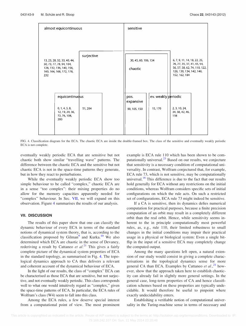
observation. Figure 4 summarises the results of our analysis.

VII. DISCUSSION

The results of this paper show that one can classify the

dynamic behaviour of every ECA in terms of the standard

notions of dynamical system theory, that is, according to the

classification proposed by Gilman9 and Kurka.10 We also

determined which ECA are chaotic in the sense of Devaney,

rederiving a result by Cattaneo et al.21 This gives a fairly

complete picture of the dynamical system properties of ECA

in the standard topology, as summarised in Fig. 4. The topo-

logical dynamics approach to CA thus delivers a relevant

and coherent account of the dynamical behaviour of ECA.

In the light of our results, the class of “complex” ECA can

be characterised as those ECA that are sensitive, but not surjec-

tive, and not eventually weakly periodic. This class corresponds

well to what one would intuitively regard as “complex,” given

the space-time patterns of ECA. In particular, the ECA rules of

Wolfram’s class (W4) seem to fall into this class.

Among the ECA rules, a few deserve special interest

from a computational point of view. The most prominent

example is ECA rule 110 which has been shown to be com-

putationally universal.23 Based on our results, we conjecture

that sensitivity is a necessary condition of computational uni-

versality. In contrast, Wolfram conjectured that, for example,

ECA rule 73, which is not sensitive, may be computationally

universal.18 This difference is due to the fact that our results

hold generally for ECA without any restrictions on the initial

conditions, whereas Wolfram considers specific sets of initial

configurations on which the rule acts. On such a restricted

set of configurations, ECA rule 73 might indeed be sensitive.

If a CA is sensitive, then its dynamics defies numerical

computation for practical purposes, because a finite precision

computation of an orbit may result in a completely different

orbit than the real orbit. Hence, while sensitivity seems in-

herent to the in principle computationally most powerful

rules, as, e.g., rule 110, their limited robustness to small

changes in the initial conditions may impair their practical

usage in a physical or biological system: Even a single bit-

flip in the input of a sensitive ECA may completely change

the computed output.

Among the many questions left open, a natural exten-

sion of our study would consist in giving a complete charac-

terisations in the topological dynamics sense for more

general CA than ECA. Examples by Cattaneo et al.,21 how-

ever, show that the approach taken here to establish chaotic-

ity can already fail in slightly more general settings. In the

general case, long-term properties of CA and hence classifi-

cation schemes based on these properties are typically unde-

cidable. It would therefore be useful to pinpoint where

exactly undecidability enters.

Establishing a verifiable notion of computational univer-

sality in the Turing-machine sense in terms of necessary and

FIG. 4. Classification diagram for the ECA. The chaotic ECA are inside the double-framed box. The class of the sensitive and eventually weakly periodic

ECA is not complete.

043143-9 M. Sch€ule and R. Stoop Chaos 22, 043143 (2012)

This article is copyrighted as indicated in the article. Reuse of AIP content is subject to the terms at: http://scitation.aip.org/termsconditions. Downloaded to IP:

79.169.242.107 On: Sun, 11 May 2014 23:20:48

sufficient conditions related to the dynamic behaviour of the

underlying system would greatly advance our understanding

of the relation between computational and dynamic properties

of physical and biological systems. Part of the problem to clar-

ify this relation is that there is no unanimous accepted defini-

tion of computational universality for computational systems

such as CA (see, e.g., the discussion by Ollinger24 and Delv-

enne et al.25 Delvenne et al. also prove necessary conditions

for a symbolic system to be universal, according to their defi-

nition of universality, and demonstrate the existence of a uni-

versal and chaotic system on the Cantor space.). To different

definitions of universality, there might thus correspond to dif-

ferent topological dynamics properties. Despite this fact, we

conjecture that for ECA sensitivity and non-surjectivity are

necessary conditions of universality. This conjecture is in ac-

cordance with the intuitive idea that systems at the “edge of

chaos,” i.e., systems with neither too simple nor chaotic dy-

namical behaviour, are the computationally relevant systems

for biology. Such intermittent systems have, moreover, been

characterised as having the largest complexity in the sense

that their behaviour is the hardest to predict.26 If computation

is measured as a reduction of complexity,27 the intermittent

systems may then be said to provide the complexity needed

for efficient computations.

The extension of the results and observations from ECA

to general one-dimensional CA or higher-dimensional CA is

thus not without problems. Being much more tractable, ECA

provide an important benchmark to test ideas on universality,

the “edge of chaos” hypothesis and, generally, on how

“computation” occurs in nature.

ACKNOWLEDGMENTS

The authors wish to thank Jarkko Kari for helpful com-

ments and advice.

This work was partly supported by ETH Research Grant

No. TH-04 07-2 and the cogito foundation.

1M. Sipser, Introduction to the Theory of Computation (International

Thompson Publishing, 1996).2C. H. Papadimitriou, Computational Complexity (John Wiley and Sons

Ltd., 2003).3G. A. Hedlund, “Endomorphisms and automorphisms of the shift dynami-

cal system,” Theory Comput. Syst. 3(4), 320–375 (1969).

4S. Wolfram, “Cellular automata,” Los Alamos Sci. 9(2–21), 2–27 (1983).5S. Wolfram, “Statistical mechanics of cellular automata,” Rev. Mod. Phys.

55(3), 601–644 (1983).6S. Wolfram, “Universality and complexity in cellular automata,” Physica

D 10(1–2), 1–35 (1984).7W. Li and N. Packard, “The structure of the elementary cellular automata

rule space,” Complex Syst. 4(3), 281–297 (1990).8K. Culik and S. Yu, “Undecidability of CA classification schemes,” Com-

plex Syst. 2(2), 177–190 (1988).9R. H. Gilman, “Classes of linear cellular automata,” Ergod. Theory Dyn.

Syst. 7, 105–118 (1987).10P. Kurka, “Languages, equicontinuity and attractors in cellular automata,”

Ergod. Theory Dyn. Syst. 17(02), 417–433 (2001).11P. Kurka, Topological and Symbolic Dynamics, Vol. 11 (Soci�et�e

Math�ematique de France, 2003).12B. Durand, E. Formenti, and G. Varouchas, “On undecidability of equicon-

tinuity classification for cellular automata,” Discrete Math. Theor. Com-

put. Sci. AB(DMCS), 117–128 (2003).13O. Martin, A. M. Odlyzko, and S. Wolfram, “Algebraic properties of cellu-

lar automata,” Commun. Math. Phys. 93(2), 219–258 (1984).14L. O. Chua, S. Yoon, and R. Dogaru, “A nonlinear dynamics perspective

of Wolframs new kind of science. Part I: Threshold of complexity,” Int. J.

Bifurcation Chaos 12(12), 2655–2766 (2002).15M. Sch€ule, T. Ott, and R. Stoop, “Global dynamics of finite cellular

automata,” In Artificial Neural Networks, ICANN 2008 (2008), pp. 71–

78.16H. Betel and P. Flocchini, “On the relationship between boolean and

fuzzy cellular automata,” Electron. Notes Theor. Comput. Sci. 252, 5–21

(2009).17E. Mendelson, Introduction to Mathematical Logic (Chapman & Hall/

CRC, 1997).18S. Wolfram, A New Kind of Science (Wolfram Media, 2002).19P. Kurka, “Topological dynamics of one-dimensional cellular automata,”

In Mathematical Basis of Cellular Automata, Encyclopedia of Complexityand System Science (Springer-Verlag, 2008).

20R. L. Devaney, An Introduction to Chaotic Dynamical Systems (Westview,

2003).21G. Cattaneo, M. Finelli, and L. Margara, “Investigating topological chaos

by elementary cellular automata dynamics,” Theor. Comput. Sci. 244(1–

2), 219–241 (2000).22F. Blanchard and P. Tisseur, “Some properties of cellular automata

with equicontinuity points,” Ann. I.H.P. Probab. Stat. 36(5), 569–582

(2000).23M. Cook, “Universality in elementary cellular automata,” Complex Syst.

15(1), 1–40 (2004).24N. Ollinger, “Universalities in cellular automata: A (short) survey,” Pro-

ceedings of the First Symposium on Cellular Automata ‘Journ�ees Auto-mates Cellulaires’, 102–118 (2008).

25J. C. Delvenne, P. Kurka, and V. Blondel, “Decidability and universality

in symbolic dynamical systems,” Fund. Inform. 74(4), 463–490 (2006).26R. Stoop, N. Stoop, and L. Bunimovich, “Complexity of dynamics as vari-

ability of predictability,” J. Stat. Phys. 114(3), 1127–1137 (2004).27R. Stoop and N. Stoop, “Natural computation measured as a reduction of

complexity,” Chaos 14, 675 (2004).

043143-10 M. Sch€ule and R. Stoop Chaos 22, 043143 (2012)

This article is copyrighted as indicated in the article. Reuse of AIP content is subject to the terms at: http://scitation.aip.org/termsconditions. Downloaded to IP:

79.169.242.107 On: Sun, 11 May 2014 23:20:48